Determination of Helmert transformation parameters for continuous GNSS networks: a case study of the Géoazur GNSS network

ABSTRACT

In this paper, we propose an approach to determine seven parameters of the Helmert transformation by transforming the coordinates of a continuous GNSS network from the World Geodetic System 1984 (WGS84) to the International Terrestrial Reference Frame. This includes (1) converting the coordinates of common points from the global coordinate system to the local coordinate system, (2) identifying and eliminating outliers by the Dikin estimator, and (3) estimating seven parameters of the Helmert transformation by least squares (LS) estimation with the “clean” data (i.e. outliers removed). Herein, the local coordinate system provides a platform to separate points’ horizontal and vertical components. Then, the Dikin estimator identifies and eliminates outliers in the horizontal or vertical component separately. It is significant because common points in a continuous GNSS network may contain outliers. The proposed approach is tested with the Géoazur GNSS network with the results showing that the Dikin estimator detects outliers at 6 out of 18 common points, among which three points are found with outliers in the vertical component only. Thus, instead of eliminating all coordinate components of these six common points, we only eliminate all coordinate components of three common points and only the vertical component of another three common points. Finally, the classical LS estimation is applied to “clean” data to estimate seven parameters of the Helmert transformation with a significant accuracy improvement. The Dikin estimator’s results are compared to those of other robust estimators of Huber and Theil-Sen, which shows that the Dikin estimator performs better. Furthermore, the weighted total least-squares estimation is implemented to assess the accuracy of the LS estimation with the same data. The inter-comparison of the seven estimated parameters and their standard deviations shows a small difference at a few per million levels (E-6).

KEYWORDS:

• Continuous GNSS
• tectonic geodesy
• Dikin estimation
• Helmert transformation

1. Introduction

Global Navigation Satellite System (GNSS) networks for monitoring the movement of the Earth’s crust have been actively developed in many countries or regions with seismic activities, such as Japan (Ito, Takahashi, and Ohzono 2019), Turkey (Uzel et al. 2013), China (Yao 2003), Australia (El-Mowafy and Bilbas 2016; Woodgate et al. 2017). In fact, GNSS networks are expanding in terms of spatial scale and data storage, which causes a big challenge for processing the position time series of GNSS stations with high accuracy. This raises the demand for developing robust algorithms for data processing. In GNSS data processing, an essential step is transforming coordinates of points from the World Geodetic System 1984 (WGS84) to the International Terrestrial Reference Frame (ITRF), which is an accurate and stable coordinate system in time (Rebischung et al. 2012), using the Helmert transformation (Ronen and Even-Tzur 2017). Generally, the ITRF network is updated in every 2–4 years and is provided freely on http://itrf.ensg.ign.fr/.

The Helmert transformation parameters are estimated from common points with known coordinates in both WGS84 and ITRF systems. Over time, the coordinates of common points may occur jumps caused by poor signal, antenna replacement, or earthquakes (Ming et al. 2016). Also, they may consist of gross errors (a.k.a. outliers) caused by multipath effects, site-specific error, or abnormal satellite orbits (Nikolaidis 2002). When the coordinates of common points contain outliers, the estimation results of the Helmert transformation parameters may be incorrect (Yang 1999). Consequently, the calculated coordinates of other GNSS points are incorrect as well. Therefore, it is necessary to identify and eliminate common points containing outliers before calculating Helmert transformation parameters. It allows reducing the uncertainty of GNSS stations in the ITRF as well as improving the accuracy of velocity fields of the continuous GNSS network.

Generally, to process a GNSS position time series, a classical method such as the least-squares (LS) estimation is often used to determine the Helmert transformation parameters. As an example, Tran (2021) processed GNSS data and transformed the coordinates of points to the ITRF2000 by using the Bernese software (Dach and Walser 2015), which implemented the LS estimator for calculating the parameters of the Helmert transformation. In another example, the GIPSY/OASIS software applying the LS estimator to determine the Helmert transformation parameters was employed to calculate the coordinates of monitoring stations in the IGS08 system (Rebischung et al. 2012). In a study of transformation parameter determination, only the data that did not contain outliers were used to estimate the parameters of the Helmert transformation (Watson 2006).

On the other hand, in studies of transforming the geodetic reference system by using robust estimations, a stable estimator was implemented to determine the Helmert transformation parameters based on common points, which consisted of high breakdown points (Yang 1999). The estimation results were reasonable. However, Yang’s work focused on significantly high outliers, and the transformation equation was formed in the global three-dimensional (3D) coordinate system. Also, Janicka (2011) applied the M-estimation and Hausbrand’s correction to estimate the transformation parameters. The results showed that this technique was effective when the influence of outliers was removed before transformation calculation. Similarly, the M-estimation was implemented to determine parameters of coordinate transformation to eliminate the influence of outliers during data processing as in Janicka and Rapinski (2013) and Chang, Xu, and Wang (2018). In most of these studies, the Helmert transformation parameters, which had been estimated in the previous step using M-estimation, were immediately applied to transform the coordinates of other GNSS stations. It is not optimal because the errors in those estimations do not follow the normal distribution. Therefore, we propose an approach that consists of two steps to determine the Helmert transformation parameters from common points of continuous GNSS networks. Initially, the Dikin estimator is used to detect and eliminate outliers. Then, the classical LS estimator is implemented to estimate the Helmert transformation parameters from the clean data, i.e. that does not include outliers. Also, to eliminate outliers independently in the horizontal and vertical components, both steps are performed in the local coordinate system.

The remainder of the study is organized as follows: Section 2 introduces the proposed flowchart for transforming coordinates of points from WGS84 to ITRF. Section 3 introduces the Helmert transformation calculation in a 3D coordinate system and the challenge of its implementation in a continuous GNSS network. The implementation of the Helmert transformation in a local coordinate system is shown in Section 4. In Section 5, the Dikin method to detect and eliminate outliers is presented. The dataset, results, and discussions are described in Section 6. Finally, Section 7 is the conclusion.

2. Workflow

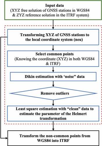
Figure 1 illustrates the steps used in transforming coordinates of points in a continuous GNSS network proposed in this study. In the first step, the GNSS data is processed by which coordinates of points are derived in WGS84. At the same time, common points are also provided in ITRF. The coordinates are then converted to the local coordinate system. As mentioned above, this is to separate the coordinates into the horizontal ($e,n$) and vertical ($u$) components. The Dikin estimator is subsequently applied to common points to detect outliers. In this way, detected outliers are removed to form “clean” data, which is then used to estimate the Helmert transformation parameters by the LS estimation. Finally, the derived parameters are utilized to transform the coordinates of other points from WGS84 to ITRF. Details on these steps will be described in the following sections.

Figure 1. Proposed flowchart for transforming coordinates of points from WGS84 to ITRF.

3. Challenge of applying the Helmert transformation to continuous GNSS observations

3.1. Helmert transformation

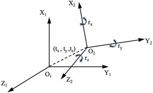
In geodesy, the Helmert transformation method is often used to transform the coordinates between two 3D coordinate systems (Chen and Wang 2009; Deakin 1998). In the Helmert transformation, two 3D coordinate systems are different in their origins, axes, and scale factor. These components are decomposed into seven parameters, including three translations of the coordinate origin along the axes (t_x, t_y, t_z), three Euler rotation angles between three axes (r_x, r_y, r_z), and the scale factor (1+k), as in Figure 2.

Figure 2. Helmert transformation between two 3D coordinate systems.

The Helmert transformation allows transforming the coordinates of points ${\left[\begin{array}{ccc}{\mathrm{X}}_1& {\mathrm{Y}}_1& {\mathrm{Z}}_1\end{array}\right]}^{\mathrm{T}}$ in the 1^st coordinate system to ${\left[\begin{array}{ccc}{\mathrm{X}}_2& {\mathrm{Y}}_2& {\mathrm{Z}}_2\end{array}\right]}^{\mathrm{T}}$ in the 2^nd coordinate system. When the Euler rotation angles are small, the Helmert transformation is interpreted following the Bursa–Wolf’s equation (Mitsakaki, Agatza-Balodimou, and Papazissi 2006):

(1) $\left[\begin{array}{c}{X}_2\\ Y_2\\ Z_2\end{array}\right]=\left(1+k\right)\left[\begin{array}{ccc}1& r_z& -r_y\\ -r_z& 1& r_x\\ r_y& -r_x& 1\end{array}\right]\left[\begin{array}{c}{X}_1\\ Y_1\\ Z_1\end{array}\right]+\left[\begin{array}{c}{t}_x\\ t_y\\ t_t\end{array}\right]$(1)

The seven parameters of the Helmert transformation model are determined based on common points with known coordinates in both systems. For a common point $i$, Equation (1)(1) $\left[\begin{array}{c}{X}_2\\ Y_2\\ Z_2\end{array}\right]=\left(1+k\right)\left[\begin{array}{ccc}1& r_z& -r_y\\ -r_z& 1& r_x\\ r_y& -r_x& 1\end{array}\right]\left[\begin{array}{c}{X}_1\\ Y_1\\ Z_1\end{array}\right]+\left[\begin{array}{c}{t}_x\\ t_y\\ t_t\end{array}\right]$(1) can be written as

(2) $\left[\begin{array}{c}{X}_2^i\\ Y_2^i\\ Z_2^i\end{array}\right]=\left(1+k\right)\left[\begin{array}{ccc}1& r_z& -r_y\\ -r_z& 1& r_x\\ r_y& -r_x& 1\end{array}\right]\left[\begin{array}{c}{X}_1^i\\ Y_1^i\\ Z_1^i\end{array}\right]+\left[\begin{array}{c}{t}_x\\ t_y\\ t_z\end{array}\right]$(2)

Equation (2)(2) $\left[\begin{array}{c}{X}_2^i\\ Y_2^i\\ Z_2^i\end{array}\right]=\left(1+k\right)\left[\begin{array}{ccc}1& r_z& -r_y\\ -r_z& 1& r_x\\ r_y& -r_x& 1\end{array}\right]\left[\begin{array}{c}{X}_1^i\\ Y_1^i\\ Z_1^i\end{array}\right]+\left[\begin{array}{c}{t}_x\\ t_y\\ t_z\end{array}\right]$(2) can then be reformed as

(3) $\left[\begin{array}{c}{X}_2^i\\ Y_2^i\\ Z_2^i\end{array}\right]=\left[\begin{array}{c}{t}_x\\ t_y\\ t_t\end{array}\right]+\left[\begin{array}{ccc}1& r_z& -r_y\\ -r_z& 1& r_x\\ r_y& -r_x& 1\end{array}\right]\left[\begin{array}{c}{\mathrm{X}}_1^i\\ {\mathrm{Y}}_1^i\\ {\mathrm{Z}}_1^i\end{array}\right]+k\left[\begin{array}{c}{\mathrm{X}}_1^i\\ {\mathrm{Y}}_1^i\\ {\mathrm{Z}}_1^i\end{array}\right]+\left[\begin{array}{c}{\mathrm{X}}_1^i\\ {\mathrm{Y}}_1^i\\ {\mathrm{Z}}_1^i\end{array}\right]$(3)

In the form of error equation, Equation (3)(3) $\left[\begin{array}{c}{X}_2^i\\ Y_2^i\\ Z_2^i\end{array}\right]=\left[\begin{array}{c}{t}_x\\ t_y\\ t_t\end{array}\right]+\left[\begin{array}{ccc}1& r_z& -r_y\\ -r_z& 1& r_x\\ r_y& -r_x& 1\end{array}\right]\left[\begin{array}{c}{\mathrm{X}}_1^i\\ {\mathrm{Y}}_1^i\\ {\mathrm{Z}}_1^i\end{array}\right]+k\left[\begin{array}{c}{\mathrm{X}}_1^i\\ {\mathrm{Y}}_1^i\\ {\mathrm{Z}}_1^i\end{array}\right]+\left[\begin{array}{c}{\mathrm{X}}_1^i\\ {\mathrm{Y}}_1^i\\ {\mathrm{Z}}_1^i\end{array}\right]$(3) can be written as

(4) $\left[\begin{array}{c}{X}_2^i-X_1^i\\ Y_2^i-Y_1^i\\ Z_2^i-Z_1^i\end{array}\right]=\left[\begin{array}{c}{t}_x\\ t_y\\ t_t\end{array}\right]+\left[\begin{array}{ccc}1& r_z& -r_y\\ -r_z& 1& r_x\\ r_y& -r_x& 1\end{array}\right]\left[\begin{array}{c}{X}_1^i\\ Y_1^i\\ Z_1^i\end{array}\right]+k\left[\begin{array}{c}{X}_1^i\\ Y_1^i\\ Z_1^i\end{array}\right]+\left[\begin{array}{c}{v}_1^i\\ v_1^i\\ v_1^i\end{array}\right]$(4)

and can be reformed as

(5) $\left[\begin{array}{c}{X}_2^i-X_1^i\\ Y_2^i-Y_1^i\\ Z_2^i-Y_1^i\end{array}\right]=\left[\begin{array}{ccccccc}1& 0& 0& 0& -Z_1^i& Y_1^i& X_1^i\\ 0& 1& 0& Z_1^i& 0& -X_1^i& Y_1^i\\ 0& 0& 1& -Y_1^i& X_1^i& 0& Z_1^i\end{array}\right]\left[\begin{array}{c}{t}_x\\ t_y\\ t_z\\ r_x\\ r_y\\ r_z\\ k\end{array}\right]+\left[\begin{array}{c}{v}_{{ }_x}^i\\ v_{{ }_y}^i\\ v_{{ }_z}^i\end{array}\right]$(5)

Rewrite Equation (5)(5) $\left[\begin{array}{c}{X}_2^i-X_1^i\\ Y_2^i-Y_1^i\\ Z_2^i-Y_1^i\end{array}\right]=\left[\begin{array}{ccccccc}1& 0& 0& 0& -Z_1^i& Y_1^i& X_1^i\\ 0& 1& 0& Z_1^i& 0& -X_1^i& Y_1^i\\ 0& 0& 1& -Y_1^i& X_1^i& 0& Z_1^i\end{array}\right]\left[\begin{array}{c}{t}_x\\ t_y\\ t_z\\ r_x\\ r_y\\ r_z\\ k\end{array}\right]+\left[\begin{array}{c}{v}_{{ }_x}^i\\ v_{{ }_y}^i\\ v_{{ }_z}^i\end{array}\right]$(5) in the matrix form as follows:

(6) $l^i=a^i\mathrm{X}+v^i$(6)

where

$\begin{array}{rl}& l^i=\left[\begin{array}{c}{X}_2^i-X_1^i\\ Y_2^i-Y_1^i\\ Z_2^i-Y_1^i\end{array}\right];a^i=\left[\begin{array}{ccccccc}1& 0& 0& 0& -Z_1^i& Y_1^i& X_1^i\\ 0& 1& 0& Z_1^i& 0& -X_1^i& Y_1^i\\ 0& 0& 1& -Y_1^i& X_1^i& 0& Z_1^i\end{array}\right];v^i=\left[\begin{array}{c}{v}_{{ }_x}^i\\ v_{{ }_y}^i\\ v_{{ }_z}^i\end{array}\right];\\ & X={\left[\begin{array}{ccccccc}{t}_x& t_y& t_z& r_x& r_y& r_z& k\end{array}\right]}^T\end{array}$

The weight matrix, $p^i$, is calculated from the variance-covariance matrix, ${\mathrm{C}}_1^i,{\mathrm{C}}_2^i$ of the point i in the ^first and ^second coordinate systems and given as

(7) $p^i={\left[{\mathrm{C}}_1^i+{\mathrm{C}}_2^i\right]}^{-1}$(7)

Then, each common point is used to form three observation equations of the form in Equation (5)(5) $\left[\begin{array}{c}{X}_2^i-X_1^i\\ Y_2^i-Y_1^i\\ Z_2^i-Y_1^i\end{array}\right]=\left[\begin{array}{ccccccc}1& 0& 0& 0& -Z_1^i& Y_1^i& X_1^i\\ 0& 1& 0& Z_1^i& 0& -X_1^i& Y_1^i\\ 0& 0& 1& -Y_1^i& X_1^i& 0& Z_1^i\end{array}\right]\left[\begin{array}{c}{t}_x\\ t_y\\ t_z\\ r_x\\ r_y\\ r_z\\ k\end{array}\right]+\left[\begin{array}{c}{v}_{{ }_x}^i\\ v_{{ }_y}^i\\ v_{{ }_z}^i\end{array}\right]$(5) . To determine seven parameters in Equation (5)(5) $\left[\begin{array}{c}{X}_2^i-X_1^i\\ Y_2^i-Y_1^i\\ Z_2^i-Y_1^i\end{array}\right]=\left[\begin{array}{ccccccc}1& 0& 0& 0& -Z_1^i& Y_1^i& X_1^i\\ 0& 1& 0& Z_1^i& 0& -X_1^i& Y_1^i\\ 0& 0& 1& -Y_1^i& X_1^i& 0& Z_1^i\end{array}\right]\left[\begin{array}{c}{t}_x\\ t_y\\ t_z\\ r_x\\ r_y\\ r_z\\ k\end{array}\right]+\left[\begin{array}{c}{v}_{{ }_x}^i\\ v_{{ }_y}^i\\ v_{{ }_z}^i\end{array}\right]$(5) , at least three common points are needed, and the system of observation equations for n common points (n ≥ 3) is written as:

(8) $\stackrel{\sim }{\mathrm{L}}=\stackrel{\sim }{A}\mathrm{X}+\stackrel{\sim }{\mathrm{V}},\mathrm{P}$(8)

where

$L^{\%}=\left[\begin{array}{c}{l}^1\\ \dots \\ l^n\end{array}\right];A^{\%}=\left[\begin{array}{c}{a}^1\\ \dots \\ a^n\end{array}\right];V^{\%}=\left[\begin{array}{c}{v}^1\\ \dots \\ v^n\end{array}\right]P=\left[\begin{array}{c}{P}^1\dots 0\\ \dots \dots \dots \\ 0\dots p^n\end{array}\right]$

If the coordinates of common points contain accidental errors only (i.e. those remaining after removing possible mistakes and systematic errors), Equation (8)(8) $\stackrel{\sim }{\mathrm{L}}=\stackrel{\sim }{A}\mathrm{X}+\stackrel{\sim }{\mathrm{V}},\mathrm{P}$(8) is solved by the LS estimation.

(9) $\sum _{i=1}^{3n}{p}^i{v}^i{v}^i=\mathrm{m}\mathrm{i}\mathrm{n}$(9)

Finally, the Helmert transformation parameters in Equation (8)(8) $\stackrel{\sim }{\mathrm{L}}=\stackrel{\sim }{A}\mathrm{X}+\stackrel{\sim }{\mathrm{V}},\mathrm{P}$(8) can be determined as:

(10) $X={\left({\tilde{A}}^{T}P\tilde{A}\right)}^{{ }^{-1}}\left({\tilde{A}}^{T}P\tilde{L}\right)$(10)

Based on the Helmert transformation parameters, the coordinates of other points can be transformed into the 2^nd coordinate system by using Equation (1)(1) $\left[\begin{array}{c}{X}_2\\ Y_2\\ Z_2\end{array}\right]=\left(1+k\right)\left[\begin{array}{ccc}1& r_z& -r_y\\ -r_z& 1& r_x\\ r_y& -r_x& 1\end{array}\right]\left[\begin{array}{c}{X}_1\\ Y_1\\ Z_1\end{array}\right]+\left[\begin{array}{c}{t}_x\\ t_y\\ t_t\end{array}\right]$(1) .

3.2. Challenge of coordinate transformation in a continuous GNSS network

As mentioned above, common points used in the transformation of the coordinates of continuous GNSS stations from WGS84 to the ITRF may include abnormal values, i.e. jumps (offsets) or outliers. The offsets are typically caused by ground subsidence, earthquakes, or GNSS antenna replacement (Ming et al. 2016). The outliers are often caused by weather noise or the failure of the algorithm used in GNSS data processing (Nikolaidis 2002). The coordinates of common points are used to estimate 7 parameters of the Helmert transformation based on the LS estimation. If outliers appear in these points, the transformation results will be incorrect. Therefore, it is necessary to identify and remove common points containing outliers before estimating the Helmert transformation parameters.

On the other hand, the number of common points in continuous GNSS networks is usually limited, and thus if many common points with outliers are detected and eliminated then the minimum requirement of the number of common points used to solve Equations (8)(8) $\stackrel{\sim }{\mathrm{L}}=\stackrel{\sim }{A}\mathrm{X}+\stackrel{\sim }{\mathrm{V}},\mathrm{P}$(8) may not be met. Consequently, the aim of transforming the coordinates of continuous GNSS networks cannot complete. To meet the demand for solving Equation (8)(8) $\stackrel{\sim }{\mathrm{L}}=\stackrel{\sim }{A}\mathrm{X}+\stackrel{\sim }{\mathrm{V}},\mathrm{P}$(8) based on the LS estimation, it will be conducted in a local coordinate system, which allows separating the horizontal and vertical components. In this way, only the component that contains outliers is removed before estimating the 7 parameters of the Helmert transformation.

4. Helmert transformation in a local coordinate system

On the global scale, the velocity field of GNSS stations is continuously calculated according to the coordinate components of X, Y, and Z. Locally, it is described and determined in the directions of North-South, East-West, and upward-downward, which can be represented in the coordinate components of e, n, and u (Cox and Hart 2009). Thus, to calculate the velocity field of continuous GNSS stations in a local coordinate system, the coordinates of those points, which were previously transformed into ITRF, shall be converted to the local coordinates ($n,e,u$) as in Figure 3.

Figure 3. Global coordinate system and the local coordinate system.

The local coordinates ${\left[\begin{array}{ccc}{e}^i& n^i& u^i\end{array}\right]}^{\mathrm{T}}$ and the 3D coordinates ${\left[\begin{array}{ccc}{X}^i& Y^i& Z^i\end{array}\right]}^{\mathrm{T}}$ of a point i^th in ITRF can be transformed to each other by (Tran 2013):

(11) $\left[\begin{array}{c}{e}^i\\ n^i\\ u^i\end{array}\right]=R\left[\begin{array}{c}{X}^i-X_0\\ Y^i-Y_0\\ Z^i-Z_0\end{array}\right]$(11)

(12) $\left[\begin{array}{c}{X}^i\\ Y^i\\ Z^i\end{array}\right]=R^{-1}\left[\begin{array}{c}{e}^i\\ n^i\\ u^i\end{array}\right]+\left[\begin{array}{c}{X}_0\\ Y_0\\ Z_0\end{array}\right]$(12)

The variance-covariance matrix is transformed as

(13) $C_{enu}=R{C}_{xyz}{R}^{\mathrm{T}}$(13)

where the rotation matrix is represented by

(14) $R=\left[\begin{array}{ccc}-\mathrm{s}\mathrm{i}\mathrm{n}{\lambda }_0& \mathrm{c}\mathrm{o}\mathrm{s}{\lambda }_0& 0\\ -\mathrm{s}\mathrm{i}\mathrm{n}{\phi }_0\mathrm{c}\mathrm{o}\mathrm{s}{\lambda }_0& \mathrm{s}\mathrm{i}\mathrm{n}{\phi }_0\mathrm{s}\mathrm{i}\mathrm{n}{\lambda }_0& \mathrm{c}\mathrm{o}\mathrm{s}{\lambda }_0\\ \mathrm{c}\mathrm{o}\mathrm{s}{\phi }_0\mathrm{c}\mathrm{o}\mathrm{s}{\lambda }_0& \mathrm{c}\mathrm{o}\mathrm{s}{\phi }_0\mathrm{s}\mathrm{i}\mathrm{n}{\lambda }_0& \mathrm{s}\mathrm{i}\mathrm{n}{\phi }_0\end{array}\right]$(14)

and ${\left[\begin{array}{ccc}{X}_0& Y_0& Z_0\end{array}\right]}^{\mathrm{T}}$ and $\left({\phi }_0,{\lambda }_0\right)$ are the global 3D coordinates and the latitude, longitude of the central point of the GNSS network. The differences of the coordinates of the common point i^th between the first andsecond coordinate systems are determined as

(15) $\left[\begin{array}{c}{X}_2^i-X_1^i\\ Y_2^i-Y_1^i\\ Z_2^i-Z_1^i\end{array}\right]=\left({\mathrm{R}}^{-1}\left[\begin{array}{c}{e}_2^i\\ n_2^i\\ u_2^i\end{array}\right]+\left[\begin{array}{c}{X}_0\\ Y_0\\ Z_0\end{array}\right]\right)-\left({\mathrm{R}}^{-1}\left[\begin{array}{c}{e}_1^i\\ n_1^i\\ u_1^i\end{array}\right]+\left[\begin{array}{c}{X}_0\\ Y_0\\ Z_0\end{array}\right]\right)$(15)

Or

(16) $\left[\begin{array}{c}{X}_2^i-X_1^i\\ Y_2^i-Y_1^i\\ Z_2^i-Z_1^i\end{array}\right]=R^{-1}\left[\begin{array}{c}{e}_2^i-e_1^i\\ n_2^i-n_1^i\\ u_2^i-u_1^i\end{array}\right]$(16)

and

(17) $\left[\begin{array}{c}{e}_2^i-e_1^i\\ n_2^i-n_1^i\\ u_2^i-u_1^i\end{array}\right]=R\left[\begin{array}{c}{X}_2^i-X_1^i\\ Y_2^i-Y_1^i\\ Z_2^i-Z_1^i\end{array}\right]$(17)

or reform Equation (16)(16) $\left[\begin{array}{c}{X}_2^i-X_1^i\\ Y_2^i-Y_1^i\\ Z_2^i-Z_1^i\end{array}\right]=R^{-1}\left[\begin{array}{c}{e}_2^i-e_1^i\\ n_2^i-n_1^i\\ u_2^i-u_1^i\end{array}\right]$(16) :

(18) $l_{enu}^i=R{l}^i$(18)

where

$l_{enu}^i=\left[\begin{array}{c}{e}_2^i-e_1^i\\ n_2^i-n_1^i\\ u_2^i-u_1^i\end{array}\right];l^i=\left[\begin{array}{c}{X}_2^i-X_1^i\\ Y_2^i-Y_1^i\\ Z_2^i-Z_1^i\end{array}\right]$

Using Equation (17)(17) $\left[\begin{array}{c}{e}_2^i-e_1^i\\ n_2^i-n_1^i\\ u_2^i-u_1^i\end{array}\right]=R\left[\begin{array}{c}{X}_2^i-X_1^i\\ Y_2^i-Y_1^i\\ Z_2^i-Z_1^i\end{array}\right]$(17) , we can rewrite Equation (6)(6) $l^i=a^i\mathrm{X}+v^i$(6) in the local coordinate system as

(19) $l_{enu}^i=a_{enu}^{i}X+v_{enu}^i$(19)

where $a_{enu}^i=R{a}^i$.

In this study, we propose to use Equation (18)(18) $l_{enu}^i=R{l}^i$(18) that replaces Equation (6)(6) $l^i=a^i\mathrm{X}+v^i$(6) in estimating the Helmert transformation parameters. Indeed, Equation (18)(18) $l_{enu}^i=R{l}^i$(18) is written in the local coordinate system that allows separating the coordinate components into the horizontal (e, n) and vertical (u) as mentioned above. In this way, we can remove the equation of vertical components if only that part contains outliers, while the equations of horizontal components remain. If the outliers exist in either of the horizontal components, all three coordinate components of that point must be eliminated. It is useful when the number of the common points is small but outliers only exist in the vertical component. This is a normal phenomenon in continuous GNSS networks due to the antenna change.

5. Dikin estimator

Generally, to determine model or regression parameters when the number of measurements is larger than the number of variables, the classical LS estimation is implemented. However, the LS estimation cannot help eliminate the influence of outliers, which may appear in the observations. Therefore, statistical methods and robust estimations are implemented to identify outliers. To detect outliers from the GNSS position time series, statistical methods such as the Student test or the Fisher–Snedeker test are usually used, but they are reported not suitable for processing big data as well as have difficulty in identifying common points that contain outliers. Additionally, these statistical tests are only helpful when the number of measurements that consist of outliers is small. The Detection, Identification, and Adaptation (DIA) method, which combines estimation and testing, was proposed for detection, identification, and adaptation of model misspecifications (Kok 1984; Teunissen 2018). This method overcomes the disadvantages of the statistical methods. However, for eliminating outliers’ effects in the coordinates of common points in a continuous GNSS network, it is not optimal. In contrast, to eliminate outliers in a linear equation system, it is better to apply robust estimations (Janicka 2011; Yang 1999). This technique allows isolating outliers, adjusting data, and providing the results without the influence of outliers. In geodetic or GNSS applications, those robust estimations could be M-estimations (Chang, Xu, and Wang 2018; Janicka and Rapinski 2013), such as the Huber estimation (Huber 1992), the Theil-Sen estimation (Wang et al. 2009; Wilcox and Clark 2014).

Figure 4 shows an example of estimation results of the LS and robust estimations. It indicates that the fitting line of the LS estimation might not be sensitive to outliers, while the straight-line fitting of robust estimation methods represents the accurate determination of the central path position. This demonstrates the capability of robust estimation methods for identifying and isolating outliers in measurement data. In this study, we apply a robust estimation, which is called the Dikin estimator. This estimator follows the L1 norm and can simplify the calculation. As a result, the computation can be four times faster than the classical simplex method (Khodabandeh and Amiri-Simkooei 2011).According to Khodabandeh and Amiri-Simkooei (2011), the robust estimators are implemented based on the L1 norm following the condition:

Figure 4. Example of LS and robust estimation (Press et al. 1992).

(20) $\sum _{i=1}^n{p}_i\left|v_i\right|=\mathrm{m}\mathrm{i}\mathrm{n}$(20)

Herein, we will summarize the main steps of the Dikin adjustment method, which was introduced in Khodabandeh and Amiri-Simkooei (2011).

Standardize the error equations. As the initial assumption, there are m independent measurements and n unknowns in Equation (8)(8) $\stackrel{\sim }{\mathrm{L}}=\stackrel{\sim }{A}\mathrm{X}+\stackrel{\sim }{\mathrm{V}},\mathrm{P}$(8) . This equation is normalized by dividing by its standard deviation as:

(21) $V=P^{-1}\tilde{V};L=P^{-1}\tilde{L};A=P^{-1}\tilde{A}$(21)

Equation (8)(8) $\stackrel{\sim }{\mathrm{L}}=\stackrel{\sim }{A}\mathrm{X}+\stackrel{\sim }{\mathrm{V}},\mathrm{P}$(8) becomes:

(22) $L=AX+V,\hspace{0.17em}P=1$(22)

Optimize Equation (21)(21) $V=P^{-1}\tilde{V};L=P^{-1}\tilde{L};A=P^{-1}\tilde{A}$(21) with the absolute minimum conditions. The residual $v_i$ in Equation (21)(21) $V=P^{-1}\tilde{V};L=P^{-1}\tilde{L};A=P^{-1}\tilde{A}$(21) is decomposed into two positive natural numbers $u_i,\mathrm{a}\mathrm{n}\mathrm{d}{w}_i$. Therefore, if the error vector $V$ is decomposed into the vector form of two positive vectors u and w, we have:

(23) $V=u-w$(23)

Similarly, the variable vector $X$ is analyzed into two component vectors $\lambda ,\gamma$:

(24) $X=\lambda -\gamma$(24)

If we denote $x={\left[\begin{array}{ccc}\lambda & \gamma & \begin{array}{cc}u& w\end{array}\end{array}\right]}^{\mathrm{T}}$, $B={\left[\begin{array}{ccc}A& -A& \text{break}\begin{array}{cc}E& -E\end{array}\end{array}\right]}^{\mathrm{T}}$, and $f={\left[\begin{array}{ccc}{O}^{\mathrm{T}}& O^{\mathrm{T}}& \begin{array}{cc}{C}^{\mathrm{T}}& C^{\mathrm{T}}\end{array}\end{array}\right]}^{\mathrm{T}}$, with $\mathrm{E}$ being the unit matrix of the m×n size, $\mathrm{O}$ being the zero vector of size n, and $\mathrm{C}$ being the unit vector of size m then Equation (21)(21) $V=P^{-1}\tilde{V};L=P^{-1}\tilde{L};A=P^{-1}\tilde{A}$(21) becomes:

(25) $B^{\mathrm{T}}x=L$(25)

and the condition in Equation (19)(19) $l_{enu}^i=a_{enu}^{i}X+v_{enu}^i$(19) becomes:

(26) $f^{\mathrm{T}}x=\mathrm{m}\mathrm{i}\mathrm{n}$(26)

Solve the linear programming problems (24) and (25). Equation (24)(24) $X=\lambda -\gamma$(24) is solved by using the iteration technique based on the central path, which allows pushing the iteration process of the interior point algorithms. Based on this theory, the solution $x^{\left(t\right)}$ is always at the center of interpolation regions, which can be achieved by applying the following scaling transformation:

(27) $\stackrel{=}{x}{D}^{-1}x;B=D^{-1}B;\stackrel{=}{f}{D}^{-1}f$(27)

where $D$ is the diagonal matrix of vector $x$ in the previous iteration. The matrix $\mathrm{D}$ is given as:

(28) $D=\left[\begin{array}{ccc}{x}_1^{\left(t\right)}& \dots & 0\\ \dots & \dots & \dots \\ 0& \dots & x_{m+n}^{\left(t\right)}\end{array}\right]$(28)

Then, the solution $x$ of the ${\left(t+1\right)}^{\mathrm{t}\mathrm{h}}$ iteration is calculated by

(29) $\check{x}\left(t+1\right)=\check{x}\left(t\right)+\alpha d$(29)

where $d$ is the directional vector, which can be calculated by

(30) $d=-{\mathrm{P}}_B^{\mathrm{\perp }}f$(30)

here

(31) $P_B^{\mathrm{\perp }}=E-B{\left(B^{\mathrm{T}}B\right)}^{-1}{B}^{\mathrm{T}}$(31)

$\alpha$ is chosen as

(32) $\alpha =\frac{0.9}{-\mathrm{m}\mathrm{i}\mathrm{n}\left(d\right)}$(32)

The iteration process in Equation (28)(28) $D=\left[\begin{array}{ccc}{x}_1^{\left(t\right)}& \dots & 0\\ \dots & \dots & \dots \\ 0& \dots & x_{m+n}^{\left(t\right)}\end{array}\right]$(28) is performed until the solutions of Equation (24)(24) $X=\lambda -\gamma$(24) at two successive iteration steps are less than a threshold, usually chosen as 10⁻⁶. Then, the residual vector $v$ is determined and used to identify outliers (Tran 2013).

(33) $\begin{array}{c}\left|v_n^i\right|>3\times \mathrm{m}\mathrm{e}\mathrm{d}\mathrm{i}\mathrm{a}\mathrm{n}\left(\left|v_n\right|\right)\\ \left|v_e^i\right|>3\times \mathrm{m}\mathrm{e}\mathrm{d}\mathrm{i}\mathrm{a}\mathrm{n}\left(\left|v_e\right|\right)\\ \left|v_u^i\right|>3\times \mathrm{m}\mathrm{e}\mathrm{d}\mathrm{i}\mathrm{a}\mathrm{n}\left(\left|v_u\right|\right)\end{array}$(33)

The coordinates of points consisting of outliers are eliminated before estimating the Helmert transformation parameters using the LS estimation. Also, the rows and columns of the variance-covariance matrix in Equation (13)(13) $C_{enu}=R{C}_{xyz}{R}^{\mathrm{T}}$(13) corresponding to eliminated coordinate components are removed. Then, a new variance-covariance matrix used to determine the weight matrix of “clean” data is established. As mentioned above, to retain as many observations as possible in the determination of transformation parameters, only the observation equation of the u component of a point is removed if an outlier is found in the vertical component of that point, while other components are retained in the next step. On the other hand, if at least one of the horizontal components consists of outliers, all three components are removed. The elimination of only the vertical component allows a large number of clean observations to be retained, and thus the accuracy of the Helmert transformation parameters is guaranteed.

6 Data, results, and discussion

6.1. Géoazur GNSS network

The proposed approach is tested with the determination of the seven parameters of the Helmert transformation of two continuous GNSS networks; REseau NAtional GNSS permanent (RENAG) (http://renag.unice.fr/) and Réseau GNSS permanent (RGP) (https://rgp.ign.fr/) were developed from 1997 for scientific research and Earth observation in internal and external geophysics and geodesy. These data were collected and processed by the Geoazur laboratory (https://geoazur.oca.eu/fr/acc-geoazur). In this study, they are termed the Géoazur GNSS network for short.

The locations of common points that are used to calculate the Helmert transformation parameters for the Géoazur GNSS network are shown in Figure 5. The common points are located in the area covering most of the European continent. They are used for multi-purposes such as monitoring the displacement of plate tectonics, repositioning the local ellipsoid based on ITRF, satellite orbit adjustment. The precision of the observations is mentioned in Gordon and Stein (1992), Bock et al. (1993), Haasdyk et al. (2014) and the field velocity uncertainties are described in Perez, Monico, and Chaves (2003), Bock, Prawirodirdjo, and Melbourne (2004), Vernant et al. (2014), Ming et al. (2016). In this study, the coordinates of 18 common points in the network at the 1998.0055 epoch are used. The coordinates in the WGS84 system are derived using the GAMIT/Glock software, while the ITRF coordinates are in IGS12P33.snx (https://cddis.nasa.gov/archive/gnss/products/1701/) that were also transformed to the 1998.0055 epoch which has taken the associated discontinuities file (https://itrf.ign.fr/ITRF_solutions/2008/doc/Discontinuities-IGS-I08.snx). The coordinates of 18 common points in the WGS84 and the ITRF systems are listed in Table 1.

Figure 5. The common points of the Géoazur GNSS network.

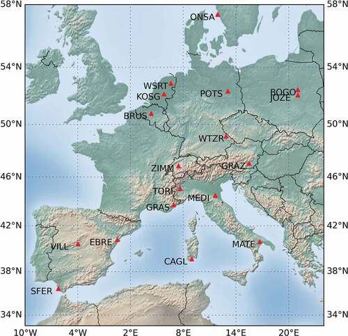
Table 1. Coordinates of 18 common points in WGS84 and ITRF at the 1998.0055 epoch.

No	Site	WGS84 at the 1998.0055 epoch			ITRF at the 1998.0055 epoch
		X/std. (m)	Y/std. (m)	Z/std (m)	X/std. (m)	Y/std. (m)	Z/std (m)
1	BOGO	3633739.0586	1397433.9842	5035353.3619	3633739.1002	1397434.0237	5035353.4151
		0.0577	0.0285	0.0541	0.0010	0.0007	0.0011
2	BRUS	4027893.7955	307045.6622	4919474.9939	4027893.8330	307045.7067	4919475.0480
		0.0573	0.0291	0.0547	0.0006	0.0005	0.0006
3	CAGL	4893378.8643	772649.6031	4004182.0082	4893378.9127	772649.6444	4004182.0786
		0.0555	0.0288	0.0566	0.0007	0.0005	0.0006
4	EBRE	4833520.1999	41536.9279	4147461.4073	4833520.2284	41536.9640	4147461.4650
		0.0556	0.0295	0.0563	0.0006	0.0005	0.0006
5	GRAS	4581690.9544	556114.6577	4389360.6542	4581690.9914	556114.6990	4389360.7107
		0.0560	0.0289	0.0558	0.0005	0.0005	0.0005
6	GRAZ	4194423.8927	1162702.5265	4647245.2804	4194423.9353	1162702.5660	4647245.3399
		0.0569	0.0286	0.0554	0.0006	0.0005	0.0006
7	JOZE	3664940.2462	1409153.7170	5009571.2743	3664940.2866	1409153.7554	5009571.3250
		0.0576	0.0285	0.0541	0.0005	0.0005	0.0005
8	KOSG	3899225.1893	396731.7815	5015078.3114	3899225.2275	396731.8256	5015078.3659
		0.0577	0.0290	0.0546	0.0005	0.0005	0.0005
9	MATE	4641949.6400	1393045.2510	4133287.3015	4641949.6814	1393045.2883	4133287.3617
		0.0552	0.0283	0.0557	0.0011	0.0007	0.0010
10	MEDI	4461400.8353	919593.3931	4449504.6311	4461400.8676	919593.4424	4449504.6934
		0.0563	0.0287	0.0557	0.0008	0.0005	0.0008
11	ONSA	3370658.6033	711876.9929	5349786.8391	3370658.6441	711877.0373	5349786.8892
		0.0587	0.0287	0.0535	0.0006	0.0005	0.0008
12	POTS	3800689.7107	882077.2331	5028791.2077	3800689.7446	882077.2733	5028791.2542
		0.0576	0.0287	0.0542	0.0004	0.0004	0.0005
13	SFER	5105519.0384	−555146.0322	3769803.2297	5105519.0543	−555145.9878	3769803.2751
		0.0779	0.0315	0.0700	0.0034	0.0024	0.0029
14	TORI	4472544.3947	601634.1739	4492545.0614	4472544.4356	601634.2137	4492545.1218
		0.0564	0.0289	0.0557	0.0034	0.0023	0.0031
15	VILL	4849833.7270	−335049.2087	4116014.7910	4849833.7689	−335049.1640	4116014.8564
		0.0536	0.0298	0.0550	0.0006	0.0005	0.0006
16	WSRT	3828735.9210	443304.7983	5064884.5841	3828735.9679	443304.8443	5064884.6461
		0.0579	0.0290	0.0545	0.0004	0.0004	0.0004
17	WTZR	4075580.6247	931853.6359	4801568.0145	4075580.6638	931853.6764	4801568.0668
		0.0572	0.0287	0.0550	0.0004	0.0004	0.0005
18	ZIMM	4331297.1146	567555.7081	4633133.7937	4331297.1557	567555.7498	4633133.8528
		0.0569	0.0290	0.0556	0.0008	0.0005	0.0008

6.2. Results and discussion

The system of equations of common points is formed and calculated in the local coordinate system. To assess the effect of outliers on the estimated results of the LS and Dikin estimations, the coordinates of the 18 common points are used to estimate the Helmert transformation parameters. The LS estimator is applied first with the weights computed from the standard deviations of coordinate components. The residuals of common points computed by the LS estimator are shown in Table 2, in which the mean horizontal (2D), vertical (up), and 3D residuals are 3.6, 8.0, and 8.8 mm, respectively, while the maximum values of the horizontal and 3D uncertainties are 12.1 mm at the MEDI station and 21.9 mm at the SFER station, respectively. Except for the east residual at MEDI, most residuals are lower than two standard deviations at the 95% of confidence level.

Table 2. Residuals of common points estimated by the LS estimation with “noisy data”.

Site	Residual e (mm)	Residual n (mm)	Residual u (mm)	2D (mm)	3D (mm)
BOGO	−1.0	0.3	−2.4	1.1	2.7
BRUS	0.8	−0.5	0.4	1.0	1.1
CAGL	0.1	−1.4	13.4	1.4	13.4
EBRE	−5.5	4.3	−5.9	7.0	9.2
GRAS	0.2	−1.1	−1.9	1.1	2.2
GRAZ	−0.7	0.3	2.3	0.7	2.4
JOZE	−1.8	−0.6	−5.4	1.9	5.7
KOSG	0.3	0.1	1.3	0.3	1.3
MATE	−0.6	−0.5	−1.5	0.8	1.7
MEDI	10.1	6.7	−1.2	12.1	12.1
ONSA	0.2	−1.3	−0.3	1.3	1.3
POTS	−1.0	−0.5	−10.1	1.1	10.2
SFER	2.2	1.6	−21.7	2.7	21.9
TORI	−1.9	−0.4	3.7	2.0	4.2
VILL	−0.7	−1.8	11.0	2.0	11.2
WSRT	1.0	−0.8	12.8	1.3	12.8
WTZR	−0.5	−1.9	−3.5	1.9	4.0
ZIMM	−0.6	−0.8	4.0	1.0	4.1

Mean residuals: 2D: 3.6 mm; 3D: 8.8 mm

Mean residuals: East: 2.9 mm; North: 2.1 mm; Up: 8.0 mm

Max 2D residual: 12.1 mm at MEDI; Min 2D residual: 0.3 mm at KOSG

Max 3D residual: 21.9 mm at SFER; Min 3D residual: 1.1 mm at BRUS

The Dikin estimator is then applied to detect and eliminate outliers from the “noisy” data, with the residuals of the coordinates of common points shown in Table 3. From the table, the median residuals of the east, north, and up components are 0.65, 0.75, and 3.05 mm, respectively, and the maximum residuals are 10.3, 6.7, and 27.6 mm for the east, north, and up uncertainties, respectively. By implementing the condition in Equation (27)(27) $\stackrel{=}{x}{D}^{-1}x;B=D^{-1}B;\stackrel{=}{f}{D}^{-1}f$(27) with the threshold in Equation (32)(32) $\alpha =\frac{0.9}{-\mathrm{m}\mathrm{i}\mathrm{n}\left(d\right)}$(32) , 6 common points containing outliers are identified and noted in the last column of Table 3. Specifically, 10 out of 54 coordinate components (approximately 18.5%) are identified as outliers by the Dikin method, in which 3 out of 6 common points have detected outliers in the vertical component.

Table 3. Residuals of common points estimated from the Dikin estimator with “noisy” data.

Site	Residual e (mm)	Residual n (mm)	Residual u (mm)	2D (mm)	3D (mm)	Outlier
BOGO	0.0	0.9	0.0	0.9	0.9
BRUS	0.9	0.1	−1.3	0.9	1.6
CAGL	0.3	−1.7	12.5	1.7	12.6	u
EBRE	–5.8	4.3	–9.4	7.2	11.8	e, n, u
GRAS	0.1	−1.0	−3.2	1.0	3.4
GRAZ	−0.2	0.5	3.4	0.5	3.4
JOZE	−0.7	0.0	−3.0	0.7	3.1
KOSG	0.5	0.8	0.0	1.0	1.0
MATE	0.1	−0.7	0.0	0.7	0.7
MEDI	10.3	6.7	−1.2	12.3	12.4	e, n
ONSA	1.0	−0.2	−0.1	1.0	1.1
POTS	−0.4	0.1	–9.6	0.4	9.6	u
SFER	2.0	1.6	–27.6	2.6	27.7	e, u
TORI	−1.9	−0.2	2.6	1.9	3.3
VILL	−1.0	−1.7	6.2	2.0	6.6
WSRT	1.2	0.0	11.7	1.2	11.8	u
WTZR	−0.1	−1.4	−3.1	1.5	3.4
ZIMM	−0.6	−0.5	2.9	0.7	3.0

Median of absolute east residual: 0.65 mm; max: 10.3 mm at MEDI

Median of absolute north residual: 0.75 mm; max: 6.7 mm at MEDI

Median of absolute up residual: 3.05 mm; max: 27.6 mm at SFER

As shown in Table 3, the outliers are identified in the CAGL, EBRE, MEDI, POST, SFER, and WSRT stations, in which the outliers in the horizontal components are found at EBRE, MEDI, and SFER. Therefore, all coordinate components of these points are eliminated in the following step. Meanwhile, the outliers in the vertical component only (u) are found at CAGL, POTS, and WSRT, and thus the horizontal (n and e) components of these points are retained, i.e. only the u components are removed in the next step. Totally, 12 coordinates (approximately 22.2%) are removed before implementing the LS estimator. As a result, 42 coordinates from 15 common points that do not contain outliers (i.e. “clean” data) are used to estimate 7 parameters of the Helmert transformation by using the LS estimation. This is the core in the proposed approach in this study to estimate the Helmert transformation parameters with high accuracy, in which the Dikin and LS estimators are combined into a flowchart as shown in Figure 1. The residuals of the estimated results are shown in Table 4 and the estimated parameters are shown in the 2^nd column of Table 5.

Table 4. Residuals of common points estimated by the LS estimation with “clean” data.

Site	Residual in e (mm)	Residual in n (mm)	Residual in u (mm)	2D (mm)	3D (mm)
BOGO	−0.2	1.2	1.8	1.2	2.2
BRUS	1.0	0.3	−2.2	1.0	2.4
CAGL	0.6	−0.9	—	1.1	—
EBRE	—	—	—	—	—
GRAS	0.3	−0.5	−4.9	0.6	4.9
GRAZ	−0.3	0.9	3.6	1.0	3.8
JOZE	−1.0	0.3	−1.2	1.0	1.6
KOSG	0.6	0.9	−0.5	1.1	1.2
MATE	0.1	0.0	−0.4	0.1	0.4
MEDI	—	—	—	—	—
ONSA	1.0	−0.2	1.1	1.0	1.5
POTS	−0.5	0.3	—	0.6	—
SFER	—	—	—	—	—
TORI	−1.8	0.2	1.3	1.8	2.3
VILL	−0.2	−1.1	2.4	1.2	2.7
WSRT	1.3	0.0	—	1.3	—
WTZR	−0.2	−1.2	−2.9	1.2	3.2
ZIMM	−0.5	−0.2	1.9	0.5	2.0

Mean residuals: 2D: 1.1 mm; 3D: 2.6 mm

Mean residuals: East: 0.8 mm; North: 0.7 mm; Up: 2.4 mm

Max 2D residual: 1.8 mm at TORI; Min 2D residual: 0.1 mm at MATE

Max 3D residual: 4.9 mm at GRAS; Min 3D residual: 0.4 mm at MATE

Table 5. Comparison of estimated Helmert transformation parameters by the least square estimation and robust estimators (ppb stands for part per billion and mas stands for milliarcsecond).

Transformation parameters	Least square estimation with “clean” data	Dikin estimator with “noisy” data	Huber estimator with “noisy” data	Theil Sen estimator with “noisy” data	Difference of estimated parameters
					LS - Dikin	LS - Huber	LS - Theil Sen
Tx (cm)	8.3	7.5	7.9	7.0	0.7	0.4	1.3
Ty (cm)	4.1	5.3	6.3	7.2	−1.2	−2.2	−3.1
Tz (cm)	5.6	6.3	8.4	3.8	−0.7	−2.9	1.7
k (ppb)	−4.3	−4.7	−5.0	−3.5	0.4	0.7	−0.8
Rx (mas)	−0.3	0.0	−0.1	0.3	−0.3	−0.2	−.6
Ry (mas)	−1.1	−0.8	−1.1	−.8	−0.3	0.0	−0.3
Rz (mas)	−0.2	−0.4	−0.5	−1.2	0.3	0.3	1.0

In Table 4, the mean values of the horizontal and vertical uncertainties derived from the LS estimator with “clean” data are 1.1 mm and 2.4 mm. The maximum residuals in the horizontal components are less than 2 mm, while that of the vertical component is 5 mm. This indicates a significant improvement in accuracy compared to the results in Table 2. Furthermore, compared with the accuracy shown in other studies by Bock et al. (1993), Perez, Monico, and Chaves (2003), Bock, Prawirodirdjo, and Melbourne (2004), El-Mowafy and Bilbas (2016) and Ronen and Even-Tzur (2017), the results in Table 4 and in the 2^nd column in Table 5 are of higher confidence. It shows the efficiency of the proposed approach in improving the precision of the Helmert transformation parameters.

To demonstrate the robustness of the Dikin estimator in eliminating outliers, we use the estimated results by the LS estimator with “clean” data as the reference results. They are subsequently compared with those computed from the Huber estimator (Huber 1992) and Theil Sen estimator (Wang et al. 2009; Wilcox and Clark 2014) with all coordinates of 18 common points (“noisy” data). The estimated results of 3 robust estimators are shown in Table 5 together with the differences in seven parameters between the three robust estimators and those of the reference results.

The Tx, Ty, and Tz comparisons in Table 5 show that the largest difference between the reference results and the Dikin estimator’s results is only 1.2 cm, while 2.9 cm and 3.1 cm are found from the differences between Huber and Theil-Sen estimators with the reference values. In contrast, the comparison of Rx, Ry and Rz shows that the results from the Dikin estimator are slightly worse than those of the Huber method, but are much better than the Theil-Sen estimator. Furthermore, the difference of the estimated k between the LS estimation and the Dikin method is only 0.4 ppb, which is approximately half of the differences between Huber’s and Theil-Sen’s results and the reference results. Overall, the 7 parameters estimated by the Dikin estimator are the closest to the reference results. This demonstrates the efficiency of the Dikin method in eliminating outliers and providing better results compared to the Huber and Theil-Sen methods.

To verify the 7 Helmert transformation parameters estimated by the LS estimation (the 2^nd column in Table 5), the weighted total least squares (WTLS) method (Amiri-Simkooei and Jazaeri 2012; Jazaeri, Amiri-Simkooei, and Sharifi 2014) is also implemented. This estimator was developed based on the LS theory with weighted matrices calculated from the variance-covariance matrix of measurements and the variance-covariance matrix of the design matrix. The estimated parameters and the associated standard deviations of the errors from the LS and WTLS methods with “clean” data are shown in Table 6. It indicates that the difference between the two results is only a few ppm in both estimated values and their standard deviations. Therefore, it can be confidently concluded that the results estimated by the LS estimation are reliable when the observations contain only random noise.

Table 6. Comparison between estimated Helmert transformation parameters of classical LS and WTLS estimation.

Helmert transformation parameters	Classical LS estimation with “clean” data		WTLS estimation with “clean” data		Difference
	Estimated	Std. error	Estimated	Std. error	Estimated (1E–6)	Std. error (1E–6)
Tx (cm)	8.26920898	0.45147637	8.26920956	0.45147620	−0.58	0.17
Ty (cm)	4.06669209	0.61247237	4.06669296	0.61247236	−0.87	0.01
Tz (cm)	5.57864163	0.45204974	5.57864084	0.45204955	0.79	0.19
k (ppb)	−4.33263704	0.48295561	−4.33263687	0.48295556	−0.17	0.05
Rx (mas)	−0.32965777	0.16412977	−0.32965752	0.16412976	−0.26	0.01
Ry (mas)	−1.10066734	0.18140474	−1.10066765	0.18140465	0.31	0.09
Rz (mas)	−0.17349495	0.14718731	−0.17349509	0.14718731	0.14	0.00

The residuals of common points computed by the LS estimation with “clean” data are the same as those by the WTLS estimation. Therefore, the statistics of coordinate residuals estimated from the WTLS estimation is not shown.

6.3. Discussion

Here, the results retrieved from the LS estimation are discussed. Using a p-value lower than 0.05, a threshold of two 3D standard deviations is chosen. From Table 2, only the 3D residual at the SFER station is over the threshold, indicating 5.6% of common points having significant errors. This means that the results from the LS estimator with original data are still reasonable. From Table 2, the mean residuals in the east, north, and up components are 2.9, 2.1, and 8.0 mm, respectively, and the mean 3D residual is 8.8 mm. This bias estimation might not meet the requirement of the common point quality as mentioned in El-Mowafy and Bilbas (2016) and Ronen and Even-Tzur (2017). To verify the necessity of outlier elimination, the residuals of common points from the LS estimator are compared with those from the Dikin estimator (see Table 3).

The Dikin estimator has been implemented with the coordinates of 18 common points in the Géoazur GNSS network. Regarding the condition in Equation (27)(27) $\stackrel{=}{x}{D}^{-1}x;B=D^{-1}B;\stackrel{=}{f}{D}^{-1}f$(27) and the threshold in Equation (32)(32) $\alpha =\frac{0.9}{-\mathrm{m}\mathrm{i}\mathrm{n}\left(d\right)}$(32) , 10(10) $X={\left({\tilde{A}}^{T}P\tilde{A}\right)}^{{ }^{-1}}\left({\tilde{A}}^{T}P\tilde{L}\right)$(10) outliers have been detected from 54 measurements, indicating approximately 18.5% of the original data of common points containing outliers. Based on the above point of view of outlier removal, we have removed 12 coordinates from 6 common points (see Table 4), i.e. approximately 22.2% of the original data. This number of outliers is quite large compared to the normal condition. Previously, the efficiency of the Dikin estimation was demonstrated in the works by Khodabandeh and Amiri-Simkooei (2011) and Zaman and Alakus (2015). The tests consisting of 12.5% and 27.0% outliers in observations were implemented and all added outliers were identified following Khodabandeh and Amiri-Simkooei (2011).

Using the results of the Dikin estimator, outliers have been found in the horizontal coordinates at EBRE, MEDI, and SFER, and in the vertical component at CAGL, POST, and WSRT (see Table 3). However, only one common point has residual values higher than two mean 3D residuals from the LS estimation. Thus, this estimation method can only be applied to the data with random noise only following the Gaussian distribution. If outliers exist in the measurements, this method will distribute them to nearby stations in the adjustment calculation instead of eliminating them. In Table 2, the residuals in the e and n components at EBRE and MEDI stations are greater than other residuals. However, the 3D residual is slightly higher than the mean 3D residual. Furthermore, the residual in the e component at SFER is lower than the mean 2D residual. Still, an outlier has been found to exist in the east component of this common point using the Dikin estimator. A similar situation has been found at the u components of CAGL and WSRT, where their residuals are lower than two times mean vertical residuals, but outliers are existent. In contrast, the residual in the u component of WILL is much bigger than the mean residual, and this may be due to the influence of outliers at EBRE. The fact is that no outlier has been identified at of WILL (Table 4).

The residuals of coordinate components containing outliers in Dikin estimation results are greater than those of the LS estimation. Similar results from the work by Khodabandeh and Amiri-Simkooei (2011) have been presented. It pointed out that those outliers have been successfully isolated by the Dikin estimator, which means that this robust estimator isolated the coordinates consisting of outliers to minimize the outliers’ effect on the estimation results of Helmert transformation parameters. In addition, two existing robust estimators, namely Huber and Theil-Sen estimators, have been implemented to assess the performance of the Dikin method. The comparison results of the Helmert transformation parameters in Table 5 show that the Dikin method outperforms the others. However, after identifying and eliminating the coordinates containing outliers, it is necessary to re-estimate the Helmert transformation parameters by the LS estimation with “clean” data. The final residual results of coordinate measurements and the estimated Helmert transformation parameters have been shown in Table 4 and in the 2^nd column of Table 5. The results in Table 4 show that the LS estimation provides more reliable results with a mean 2D residual of 1.1 mm and a mean vertical residual of 2.4 mm, which is more reasonable compared to the estimation bias in El-Mowafy and Bilbas (2016) and Bock, Prawirodirdjo, and Melbourne (2004). In addition, the minimum and maximum 3D residuals are found to be 0.4 mm and 4.9 mm at the MATE and GRAS stations, respectively.

To prove the rigorousness of the proposed approach, the estimated Helmert transformation parameters have been compared with those of the LS estimation. As shown in Table 5, there is a significant difference in the Helmert transformation parameters between the two estimation results. Also, the uncertainty of the estimated results has significantly been improved compared to the bias from the LS estimation only. This improvement is mainly contributed by two critical factors: the change in the number of coordinate measurements and the vector value of observables. It has also indicated that eliminating outliers in previous steps is genuinely correct, even when the number of observations was reduced by approximately 22.2%. Furthermore, the WTLS method has also been implemented to verify the performance of the classical LS estimator. The comparison results in the two last columns in Table 6 have indicated that the estimation results from the two methods with “clean” data are similar. Finally, the latest estimated results of Helmert transformation parameters are reliable that are only affected by accidental errors.

7. Conclusions

This paper has proposed an approach to estimate seven parameters of the Helmert coordinate transformation to transform coordinates of continuous GNSS networks from WGS84 to ITRF. The approach is implemented in a local coordinate system applying the Dikin estimator to eliminate outliers and the LS estimator to estimate parameters. The proposed approach has been tested with the Géoazur GNSS network with the main findings being:

The computation of a GNSS coordinate time series in an accurate and stable reference frame is an essential step in processing data of continuous GNSS networks as well as determining the Earth’s crust displacement. To meet the accuracy requirement of the transformed GNSS coordinates, it is necessary to estimate the Helmert transformation parameters with uncertainties as low as possible. The estimation should be implemented in a local coordinate system, which allows separating the horizontal and vertical components. In this way, it is efficient to identify if outliers only exist in the vertical component by which the horizontal components that do not consist of outliers are retained. It helps to maintain a high number of measurements to be used in Helmert transformation parameter estimation.

The Dikin estimator can identify and isolate outliers that exist in the coordinates of common points. Also, compared to the reference results, the Dikin estimator performed better than the Huber and Theil-Sen estimators. However, the Helmert transformation parameters determined from the Dikin estimator should not be used to transform the coordinates of other GNSS stations because this estimation does not distribute errors following the normal distribution. Therefore, the combination of two estimations could be more beneficial for data processing. In this approach, the Dikin estimator is used to detect and eliminate the measurements containing outliers; then, the LS estimation is adopted to estimate the optimal Helmert transformation parameters.

The estimation results indicated that the uncertainties of the Helmert transformation parameters were significantly improved compared to the results estimated using the classical least square estimation. It proved that the outliers detected by the Dikin estimation are reliable. Finally, the calculation results indicated the advantage of the proposed approach to determine the Helmert transformation parameters and process the data of continuous GNSS networks, which are used in studies related to tectonic plate movement monitoring or large-scale subsidence monitoring.

Acknowledgments

The authors gratefully thank UMR Géoazur - Campus Azur du CNRS, France, for providing the GNSS data. We acknowledge the editor and two anonymous reviewers for their useful and constructive comments that have helped us to improve the paper.

Disclosure statement

No potential conflict of interest was reported by the author(s).

Data availability statement

Some or all data, models, or code that support the findings of this study are available from the corresponding author upon reasonable request:

− Code of Helmert transformation Programe by Python.

− Free solution of Géoazur GNSS network at epoch 1998.0055.

− Reference solution of ITRF2012 IGS12P33.snx

- Discontinuity solution of ITRF2012 sonl_2012.snx

Additional information

Funding

The work was supported by the Ministry of Education and Training of Vietnam [B2020-XDA-05].

Notes on contributors

Dinh Trong Tran

Dinh Trong Tran received a PhD in Sciences of the Universe from the University of Nice Sophia Antipolis (now renamed to Côte d’Azur University), France, in 2013. He is currently a master lecturer at the Department of Geodesy and Geomatics engineering, Hanoi University of Civil Engineering, Vietnam. His current research interest is geodetic analysis and crustal deformation monitoring.

Jean-Mathieu Nocquet

Jean-Mathieu Nocquet received a PhD in GPS and Tectonics, the HDR degree (professorial thesis) from the University of Nice Sophia Antipolis, France, in 2002 and 2011, respectively. He is currently a research director at the French National Institute for Sustainable Development (IRD). His current research interest is Earthquake cycle and active deformation.

Ngoc Dung Luong

Ngoc Dung Luong received a PhD in in Sciences of the Planet and the Universe from the University of Nice, France, in 2016. He is currently a master lecturer at the Department of Geomatics and Geodesy engineering, Hanoi University of Civil Engineering, Vietnam. His current research interest is geodetic data processing and construction deformation monitoring.

Dinh Huy Nguyen

Dinh Trong Tran received a PhD in Sciences of the Universe from the University of Nice Sophia Antipolis (now renamed to Côte d’Azur University), France, in 2013. He is currently a master lecturer at the Department of Geodesy and Geomatics engineering, Hanoi University of Civil Engineering, Vietnam. His current research interest is geodetic analysis and crustal deformation monitoring.

Dinh Huy Nguyen is a lecturer at the department of Geodesy and Geomatics Engineering, Hanoi University of civil engineering (HUCE), Vietnam. He received an M.S. degree in 2020 from Changwon National University, Republic of Korea. His experience and research interests is the GNSS positioning techniques for engineering geodey.

References

- Amiri-Simkooei, A., and S. Jazaeri. 2012. “Weighted Total Least Squares Formulated by Standard Least Squares Theory.” Journal of Geodetic Science 2 (2): 113–124. doi:10.2478/v10156-011-0036-5.
- Bock, Y., D. C. Agnew, P. Fang, J. F. Genrich, B. H. Hager, T. A. Herring, K. W. Hudnut, et al. 1993. ”Detection of Crustal Deformation from the Landers Earthquake Sequence Using Continuous Geodetic Measurements.” Nature 361 (6410): 337–340. doi:10.1038/361337a0.
- Bock, Y., L. Prawirodirdjo, and T. I. Melbourne. 2004. “Detection of Arbitrarily Large Dynamic Ground Motions with a Dense High-Rate GPS Network.” Geophysical Research Letters 31 (6): L06604. doi:10.1029/2003GL019150.
- Chang, G., T. Xu, and Q. Wang. 2018. “M-Estimator for the 3D Symmetric Helmert Coordinate Transformation.” Journal of Geodesy 92 (1): 47–58. doi:10.1007/s00190-017-1043-9.
- Chen, J., and J. Wang. 2009. “Orbit Fitting Based on Helmert Transformation.” Geo-Spatial Information Science 12 (2): 95–99. doi:10.1007/s11806-009-0236-7.
- Cox, A., and R. B. Hart. 2009. Plate Tectonics: How It Works. Hoboken, New Jersey, U.S: John Wiley & Sons.
- Dach, R., and P. Walser. 2015. “Bernese GNSS Software Version 5.2.”
- Deakin, R. E. 1998. “3-D Coordinate Transformations.” Surveying and Land Information Systems 58 (4): 223–234.
- El-Mowafy, A., and E. Bilbas. 2016. “Quality Control in Using GNSS CORS Network for Monitoring Plate Tectonics: A Western Australia Case Study.” Journal of Surveying Engineering 142 (2): 05015003. doi:10.1061/(ASCE)SU.1943-5428.0000157.
- Gordon, R. G., and S. Stein. 1992. “Global Tectonics and Space Geodesy.” Science 256 (5055): 333–342. doi:10.1126/science.256.5055.333.
- Haasdyk, J., N. Donnelly, C. Harrison, C. Rizos, C. Roberts, and R. Stanaway. 2014. “Options for Modernising the Geocentric Datum of Australia.” Research@ Locate 14: 72–85.
- Huber, P. J. 1992. “Robust Estimation of a Location Parameter.” In Samuel Kotz, Norman L. Johnson., Breakthroughs in Statistics, 492–518. New York: Springer.
- Ito, C., H. Takahashi, and M. Ohzono. 2019. “M.Estimation of Convergence Boundary Location and Velocity Between Tectonic Plates in Northern Hokkaido Inferred by GNSS Velocity Data.” Earth, Planets and Space 71 (1): 86. doi:10.1186/s40623-019-1065-z.
- Janicka, J. 2011. “Transformation of Coordinates with Robust M-Estimation and Modified Hausbrandt Correction.” Environmental Engineering. Proceedings of the International Conference on Environmental Engineering. ICEE, Vol. 8, Vilnius, Lithuania: Vilnius Gediminas Technical University, Department of Construction Economics & Property, 1330
- Janicka, J., and J. Rapinski. 2013. “M Split Transformation of Coordinates.” Survey Review 45 (331): 269–274. doi:10.1179/003962613X13726661625708.
- Jazaeri, S., A. R. Amiri-Simkooei, and M. A. Sharifi. 2014. “Iterative Algorithm for Weighted Total Least Squares Adjustment.” Survey Review 46 (334): 19–27. doi:10.1179/1752270613Y.0000000052.
- Khodabandeh, A., and A. R. Amiri-Simkooei. 2011. “Recursive Algorithm for L1 Norm Estimation in Linear Models.” Journal of Surveying Engineering 137 (1): 1–8. doi:10.1061/(ASCE)SU.1943-5428.0000031.
- Kok, J. J. 1984. On Data Snooping and Multiple Outlier Testing. Vol. 30. Rockville, Md: US Department of Commerce, National Oceanic and Atmospheric Administration, National Ocean Service, Charting and Geodetic Services.
- Ming, F., Y. Yang, A. Zeng, and Y. Jing. 2016. “Analysis of Seasonal Signals and Long-Term Trends in the Height Time Series of IGS Sites in China.” Science China Earth Sciences 59 (6): 1283–1291. doi:10.1007/s11430-016-5285-9.
- Mitsakaki, C., A. M. Agatza-Balodimou, and K. Papazissi. 2006. “Geodetic Reference Frames Transformations.” Survey Review 38 (301): 608–618. doi:10.1179/sre.2006.38.301.608.
- Nikolaidis, R. 2002. “Observation of Geodetic and Seismic Deformation with the Global Positioning System.” Ph.D. Thesis, University of California, San Diego, CA, USA.
- Perez, J. A. S., J. F. G. Monico, and J. C. Chaves. 2003. “Velocity Field Estimation Using GPS Precise Point Positioning: The South American Plate Case.” Journal of Global Positioning Systems 2 (2): 90–99. doi:10.5081/jgps.2.2.90.
- Press, W. H., B. P. Flannery, S. A. Teukolsky, and W. T. Vetterling. 1992. Numerical Recipes in FORTRAN 77: The Art of Scientific Computing. 2nd ed. New York: Cambridge University Press.
- Rebischung, P., J. Griffiths, J. Ray, R. Schmid, X. Collilieux, and B. Garayt. 2012. “IGS08: The IGS Realization of ITRF2008.” GPS Solutions 16 (4): 483–494. doi:10.1007/s10291-011-0248-2.
- Ronen, H., and G. Even-Tzur. 2017. “Kinematic Datum Based on the ITRF as a Precise, Accurate, and Lasting TRF for Israel.” Journal of Surveying Engineering 143 (4): 04017013. doi:10.1061/(ASCE)SU.1943-5428.0000228.
- Teunissen, P. J. G. 2018. “Distributional Theory for the DIA Method.” Journal of Geodesy 92 (1): 59–80. doi:10.1007/s00190-017-1045-7.
- Tran, D. T. 2013. “Analyse Rapide et Robuste Des Solutions GPS Pour La Tectonique.” Ph.D. Thesis, Université Nice Sophia Antipolis, France.
- Tran, D. T., Q. L. Nguyen, and D. H. Nguyen. 2021. “General Geometric Model of GNSS Position Time Series for Crustal Deformation Studies -A Case Study of CORS Stations in Vietnam.” Journal of the Polish Mineral Engineering Society 1 (2): 183–198. doi:10.29227/IM-2021-02-16.
- Uzel, T., K. Eren, E. Gulal, I. Tiryakioglu, A. A. Dindar, and H. Yilmaz. 2013. “Monitoring the Tectonic Plate Movements in Turkey Based on the National Continuous GNSS Network.” Arabian Journal of Geosciences 6 (9): 3573–3580. doi:10.1007/s12517-012-0631-5.
- Vernant, P., R. Bilham, W. Szeliga, D. Drupka, S. Kalita, A. K. Bhattacharyya, V. K. Gaur, P. Pelgay, R. Cattin, and T. Berthet. 2014. “Clockwise Rotation of the Brahmaputra Valley Relative to India: Tectonic Convergence in the Eastern Himalaya, Naga Hills, and Shillong Plateau.” Journal of Geophysical Research: Solid Earth 119 (8): 6558–6571. doi:10.1002/2014JB011196.
- Wang, X., X. Dang, H. Peng, and H. Zhang. 2009. “The Theil-Sen Estimators in Multiple Linear Regression Models.” Manuscript http://Home.Olemiss.Edu/~Xdang/Papers/MTSE.Pdf
- Watson, G. A. 2006. “Computing Helmert Transformations.” Journal of Computational and Applied Mathematics 197 (2): 387–394. doi:10.1016/j.cam.2005.06.047.
- Wilcox, R. R., and F. Clark. 2014. “Comparing Robust Regression Lines Associated with Two Dependent Groups When There is Heteroscedasticity.” Computational Statistics 29 (5): 1175–1186. doi:10.1007/s00180-014-0485-2.
- Woodgate, P., I. Coppa, S. Choy, S. Phinn, L. Arnold, and M. Duckham. 2017. “The Australian Approach to Geospatial Capabilities; Positioning, Earth Observation, Infrastructure and Analytics: Issues, Trends and Perspectives.” Geo-Spatial Information Science 20 (2): 109–125. doi:10.1080/10095020.2017.1325612.
- Yang, Y. 1999. “Robust Estimation of Geodetic Datum Transformation.” Journal of Geodesy 73 (5): 268–274. doi:10.1007/s001900050243.
- Yao, Y. 2003. “Crustal Movement Patterns of China Continent Measured by GPS.” Geo-Spatial Information Science 6 (4): 57–60. doi:10.1007/BF02826951.
- Zaman, T., and K. ALAKUŞ. 2015. “Some Robust Estimation Methods and Their Applications.” Alphanumeric Journal 3 (2): 73–82. doi:10.17093/aj.2015.3.2.5000152703.