AdaFI-FCN: an adaptive feature integration fully convolutional network for predicting driver’s visual attention

ABSTRACT

Visual Attention Prediction (VAP) is widely applied in GIS research, such as navigation task identification and driver assistance systems. Previous studies commonly took color information to detect the visual saliency of natural scene images. However, these studies rarely considered adaptively feature integration to different geospatial scenes in specific tasks. To better predict visual attention while driving tasks, in this paper, we firstly propose an Adaptive Feature Integration Fully Convolutional Network (AdaFI-FCN) using Scene-Adaptive Weights (SAW) to integrate RGB-D, motion and semantic features. The quantitative comparison results on the DR(eye)VE dataset show that the proposed framework achieved the best accuracy and robustness performance compared with state-of-the-art models (AUC-Judd = 0.971, CC = 0.767, KL = 1.046, SIM = 0.579). In addition, the experimental results of the ablation study demonstrated the positive effect of the SAW method on the prediction robustness in response to scene changes. The proposed model has the potential to benefit adaptive VAP research in universal geospatial scenes, such as AR-aided navigation, indoor navigation, and street-view image reading.

KEYWORDS:

• Visual Attention Prediction (VAP)
• feature integration
• Fully Convolutional Network (FCN)
• driving environment
• deep learning

1. Introduction

Visual Attention Prediction (VAP) is a task for computer vision to detect the key area of human selective visual focus. Visual attention is crucial for GIS research, especially in the field of navigation task identification (Liao et al. 2019) and driver assistance systems (Miura et al. 2005), it is determined by the visual saliency of the scene and task-driven factors (Borji, Sihite, and Itti 2012). Predicting the driver’s visual attention by real-time processing of the geospatial cues is beneficial for training novice drivers and providing visual suggestions to experienced drivers during the driving process (Deng et al. 2016; Lateef, Kas, and Ruichek 2022).

With the rapid development of the Convolutional Neural Network (CNN), several CNN-based frameworks were proposed to recognize image patterns, such as LeNet5 (Lecun et al. 1998), AlexNet (Krizhevsky, Sutskever, and Hinton 2012), and VGG (Simonyan and Zisserman 2015). Furthermore, based on the original CNN framework, the Fully Convolutional Network (FCN), such as U-Net (Ronneberger, Fischer, and Brox 2015) and the Deeplab framework (Chen et al. 2018), use the decoding block to predict the visual saliency of natural scenes and to simulate human’s visual attention in specific tasks. However, the above models didn’t consider the particularities of the driving environment, the limitation lies two fold. On the one hand, most of the previous studies focused on free-viewing visual attention, simply taking RGB features to predict visual saliency on natural scenes. Compared to free-viewing, driving is a complex and dynamic task. In general, three main characteristics in driving tasks, including stereoscopic (Lang et al. 2012), dynamic (Zhan and Dong 2021), and task-driven (Oliva et al. 2003) affect human visual attention. When transferring these universal models to the driving environment that we focus on, these intuitive and fundamental factors may be ignored. Thus, it is vital to extract features that represent these factors and integrate them into the prediction model. On the other hand, most of the previous studies failed to predict robustly by adaptive integration of multibranch prediction response to the changes of the scene. The former studies simply add up multibranch output features to make a final prediction, which did not reflect the relative importance of different features (Itti, Koch, and Niebur 1998; Palazzi et al. 2019). Note that the scene condition, such as weather, brightness, and road scenarios, influences the driver’s visual attention as well as the relative importance of multibranch features (Konstantopoulos, Chapman, and Crundall 2010; Gershon, Ben-Asher, and Shinar 2012), but existing research lacks considering the scene factors when designing the feature integration strategy. In conclusion, there remains a gap in predicting driver’s visual attention in the feature adaptive integration, especially considering the task-related characteristics and the changeable environment.

The motivation of this article is to integrate multibranch features and adaptively predict the driver’s visual attention. We obtain depth, optical flow, and semantic features from the original RGB image feature to represent stereoscopic, dynamic, and task-driven characteristics of driving tasks, then we propose an Adaptive Feature Integration Fully Convolutional Network (AdaFI-FCN) based on an FCN (see Figure 1(a)). The AdaFI-FCN framework contains three independent sub-FCNs for extracting visual attention features from each branch of input features, and an optimizer for adaptive environment weights to sum up the output results of each sub-FCN. Inspired by the VGG and the Deeplab framework, the sub-FCN consists of an encoder block, an Atrous Spatial Pyramid Pooling (ASPP) block, and a decoder block, improving the prediction accuracy by extracting and integrating multiscale image features. The Scene-Adaptive Weights (SAW) are used for the integration of three sub-FCNs’ predictions, which enable the model to better cope with the changes of the scene and improve its robustness. The proposed model has been tested on the DR(eye)VE dataset, which is a visual attention dataset for driving tasks, and it achieved state-of-the-art on accuracy and robustness.

The remainder of this paper is organized as follows. In Section 2, we describe some related works, including studies on scene factors influencing visual attention and the progress of visual attention modeling research. In Section 3, we introduce the processing of original features and then show the AdaFI-FCN framework architecture. In Section 4, we report experimental setups and results on the proposed model, including the comparison with state-of-the-art models and ablation studies. In Section 5, we discuss the contribution of SAW and our work to improve prediction efficiency. Finally, we summarize the conclusion in Section 6.

2. Related work

2.1. Factors influencing driver’s visual behaviors

Previous studies found that driver’s visual behaviors are affected by various factors, including brightness (Crundall, Shenton, and Underwood 2004), weather (Calsavara, Junior, and Larocca 2021), road condition (Richardson and Marottoli 2003), and driving speed (Liu, Sun, and Rong 2011), etc. These factors influence visibility conditions and traffic density, so drivers need to make specific visual responses to these various scenes (Konstantopoulos, Chapman, and Crundall 2010; Trick, Toxopeus, and Wilson 2010). The driving speed also affects the driver’s visual attention by influencing the driver’s visual field and concentration. Jo, Lee, and Lee (2014) found an inflection point for the visual field at a certain speed, at which drivers can handle the maximum visual information, while Palazzi et al. (2019) found that driver’s visual field is smaller, showing concentration in their visual behavior at a higher speed.

In conclusion, although previous studies noticed the influence of scene factors on driver’s visual attention, there’s not proper way to combine these geospatial cues into the VAP model. These works enlighten us on the complexity and diversity of driving scenes, and it is necessary to adapt prediction models in different scenes. To better integrate the influencing factors we reviewed into the model, we proposed the trainable scene-adaptive weights when training our prediction framework, to improve robustness in different driving scenes.

2.2. Visual saliency prediction (VSP) models for static images

Visual saliency prediction is a pixel-level classification task and is an important branch of computer vision technology. The theoretical basis of visual salience research is selective visual attention, extracted from the visual behavior of primates and humans (Koch and Ullman 1985). Itti, Koch, and Niebur (1998) proposed a classic calculation model and introduced a VSP task into the field of computer vision inspired by Koch and Ullman. The model was based on the feature integration theory (Treisman and Gelade 1980), extracting and integrating the multiscale color, intensity, and orientation features of the input image to calculate visual saliency. Later, a series of computational models of visual saliency were proposed based on feature integration theory, such as Graph-Based Visual Saliency (GBVS) (Harel, Koch, and Perona 2006) and Corner-Based Saliency (CORS) (Rueopas, Leelhapantu, and Chalidabhongse 2016). With the development of machine learning, the computational accuracy and efficiency of visual saliency models have been improved by the Bayesian model (Zhang et al. 2008; Tavakoli, Rahtu, and Heikkilä 2011; Garcia-Diaz et al. 2012; Bruce and Tsotsos 2010), Support Vector Machine (SVM) (Judd et al. 2009), and random contrast (Fang et al. 2017).

In recent years, a series of VSP models based on deep learning networks have been proposed. Compared with traditional computational models and machine learning models, they greatly improved the prediction accuracy with the help of large sample datasets (Jiang et al. 2015; Judd, Durand, and Torralba 2012) and classical deep learning frameworks, including FCN (Kruthiventi, Ayush, and Babu 2017; Huang et al. 2015; Wang and Shen 2018), Long Short-Term Memory (LSTM) (Cornia et al. 2018), and Generative Adversarial Network (GAN) (Pan et al. 2017). Among these frameworks, the FCN framework has advantages in handling pixel-level classification tasks. To improve the performance of the FCN framework, previous studies applied the skip-connections method to solve the degradation problem (Ronneberger, Fischer, and Brox 2015; Drozdzal et al. 2016; Huang et al. 2019) or used the ASPP block to extract multiscale image features (Kroner et al. 2020; Wang, Shen, and Jia 2019).

In conclusion, the VSP task is commonly solved by machine learning and deep learning frameworks. However, with the improvement of computing power and the explosive increase of model parameters, researchers gradually choose to input single-color features to deep learning models without feature engineering (Bengio, Courville, and Vincent 2013). Note that in a specific task context, it is worthwhile to extract and integrate task-related features, which benefit the prediction performance. However, only a few studies have attempted to apply feature integration theory to modify deep learning models, which were frequently used for semantic segmentation (Ning et al. 2019), remote sensing image processing (Wang, Zou, and Cai 2020), and object detection tasks (Wang et al. 2017). Based on the feature integration theory in machine learning and the FCN framework in deep learning, we extract and integrate multistream driving-related image-format features into the proposed model.

2.3. Predicting visual attention in driving tasks

Different from VSP models, visual attention should be predicted according to specific tasks (Borji, Sihite, and Itti 2012). The driving task is carried out in a stereoscopic and dynamic scene, and the driver’s visual attention is affected by task-related factors, and multistream features related to these factors should be considered. In the following part, we review the related work in three aspects: stereoscopic feature extraction, spatio-temporal feature extraction, and driving-related feature extraction.

In the field of stereoscopy, some studies have used RGB-D information to improve prediction effects. Fang et al. (2014) extracted and fused four types of features, including color, luminance, texture, and depth, to enhance the prediction of saliency maps. By adding depth features to the CNN, Leifman et al. (2017) achieved a performance 15% better than that of other video visual saliency models. Cellular automata (Wang and Wang 2017; Guo, Ren, and Bei 2016), random forest (Song et al. 2017), and CNN (Han et al. 2018) frameworks for salient object detection also improve accuracy by extracting foreground objects by introducing depth maps.

Dynamic visual attention is common and important in human routines (Wang, Shen, and Jia 2019). Previous researchers introduced optical flow images (Bak et al. 2018; Lai et al. 2020; Fang et al. 2014) and frame stacks in a certain time window (Zhou et al. 2018; Xue, Sun, and Liang 2022) in video saliency detection tasks to improve Inferring shared the performance. In addition, the LSTM framework has been widely applied to integrate spatio-temporal characteristics (Jiang et al. 2018; Wang et al. 2018; Fan et al. 2018; Fan, Wang, Cheng, et al. 2019; Fan, Wang, Huang, et al. 2019).

Last, the driver’s visual behavior is highly task-related. When predicting driver’s visual attention, it is important to combine stimulus-driven bottom-up information, such as color and brightness (Itti, Koch, and Niebur 1998), and task-driven top-down information, such as semantic information (Henderson 2003). Part of previous VAP models in driving tasks applied the Bayesian framework (Tawari and Kang 2017) and deep CNN framework (Kang and Lee 2020), simply considering the bottom-up information. In addition, other works joined the top-down information related to driving into the model, such as road vanishing points (Deng, Yan, and Li 2018), semantic segmentation (Lateef, Kas, and Ruichek 2022), and road information of interest (Zhao et al. 2020). These additional features are demonstrated to improve the performance of VAP models, showing the advantages of the feature integration method.

We drew two conclusions from the above literature. On the one hand, these results show integrating the original color features, motion features, depth features, and high-level visual features (such as semantic features) is significant for enhancing the model performance, because these features provide additional top-down information to the prediction model rather than bottom-up information. It is worth combining these features comprehensive when predicting driver’s visual attention. On the other hand, we find that although some studies have tried to use the L^m-norm method and the Winner-Take-All mechanism (Lin et al. 2013), variance-based weights (Kwak, Ko, and Byun 2007), and feature sparse weights (Zhao and Liu 2010), even without weights (Palazzi et al. 2019) to integrate multistreams of features. However, these methods remain a gap in designing an adaptive feature integration strategy to conform to environmental changes and cause limitations in robustness.

3. Methodology

3.1. Feature extraction

Based on our review in Section 2.3, we believe that in driving environments, depth features can be introduced to represent the three-dimensional scene, motion features can be introduced to represent the spatio-temporal context, and driving-related semantic features can be introduced as high-level visual features. These additional features increase the amount of information input into the model, along with the original color features (RGB images). We extracted these features by the process shown in Figure 1(a).

The RGB-D feature contains four channels, three of which are color channels (red/green/blue). The fourth channel is generated by the depth estimation model (Godard, Mac Aodha, and Brostow 2017). This framework generated binocular stereo maps and then calculated the disparity and depth maps. The color features represented the visible environment of the driver and contained low-level stimulation, while the depth channel improved the spatial information of low-level visual features in stereoscopic scenes.

The motion feature displayed in the form of optical flow images, is generated from RGB frames containing two channels (intensity/orientation). We calculated the intensity and orientation features by the Gunnar Farneback optical flow algorithm (Farnebäck 2003), which is a commonly used algorithm for detecting the motion state of the corresponding pixels of two adjacent frames (Rogalska and Napieralski 2018; Ogasawara et al. 2020; Muddamsetty et al. 2013). The algorithm required two adjacent frames to match the pixels one-to-one and then calculated the motion intensity and orientation of each pixel pair. The intensity and orientation are stored in the format of grayscale images.

The semantic feature is a 3-channel binary image representing the high-level visual features. Visual behaviors are highly correlated with driving tasks; for example, the probabilities of fixation vary for different semantic objects outside the vehicle (Zhan and Dong 2021). In this study, we used the Google Deeplab V3+ framework (Chen et al. 2018) to extract the most three significant semantic features in the driving environment: buildings, roads, and vehicles. All three feature channels are stored as binary images.

3.2. Network architecture

The AdaFI-FCN contains two parts: three sub-FCNs for predicting separate predictions of visual attention based on three streams of features: RGB-D, motion, and semantic feature; and a feature integration network, using SAW to integrate the predictions of the sub-FCNs. The details are shown as follows.

3.2.1. Sub-FCN

Referring to the commonly used method, three streams of the feature are designed to separately input to the three sub-FCNs, preventing the fusion of different-source features in the early layer of the network. To mine the multiscale mechanism of input features, the sub-FCN adopts the classical encoding-decoding structure, containing three blocks: encoder block, ASPP block, and decoder block. The architecture is shown in Figure 1(b), while the details of the network design are shown in Table 1.

Figure 1. (a) the roadmap for extracting additional information from the original data and generating predicted maps through the AdaFI-FCN framework. (b) the structure of the sub-FCN consists of encoder block, ASPP block and decoder block.

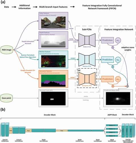
Table 1. The architecture of the sub-FCN.

Network	Layer #	Name	Operation	Stride	Padding	Dilation rate	Activation function	Output size
Input Feature	0	input	-	-	-	-	-	224 × 224 × Cinput
Encoder Block	1	conv1_1	3× 3× 64 convolution	1	SAME	1	ReLU	224 × 224×64
	2	conv1_2	3 × 3× 64 convolution	1	SAME	1	ReLU	224 × 224 × 64
	3	pool1	2 × 2 max pooling	2	-	-	-	112 × 112 ×64
	4	conv2_1	3 × 3× 128 convolution	1	SAME	1	ReLU	112 × 112 ×1 28
	5	conv2_2	3 × 3× 128 convolution	1	SAME	1	ReLU	112 × 112 × 128
	6	pool2	2 × 2 max pooling	2	-	-	-	56 × 56 × 128
	7	conv3_1	3 × 3 × 256 convolution	1	SAME	1	ReLU	56 × 56 × 256
	8	conv3_2	3 × 3 × 256 convolution	1	SAME	1	ReLU	56 × 56 × 256
	9	pool3	2 × 2 max pooling	2	-	-	-	28 × 28 × 256
	10	conv4_1	3 × 3 × 512 convolution	1	SAME	1	ReLU	28 × 28 × 512
	11	conv4_2	1 × 1 × 256 convolution	1	SAME	1	ReLU	28 × 28 × 256
ASPP Block	12-1	aspp_1	3 × 3 × 256 convolution	1	SAME	1	ReLU	28 × 28 × 256
	12-2	aspp_2	3 × 3 × 256 convolution	1	SAME	2	ReLU	28 × 28 × 256
	12-3	aspp_3	3 × 3 × 256 convolution	1	SAME	5	ReLU	28 × 28 × 256
	12-4	aspp_4	3 × 3 ×2 56 convolution	1	SAME	8	ReLU	28 × 28 × 256
	13	aspp_concat	concat Layer #12	-	-	-	-	28 × 28 × 1024
Decoder Block	14	upsample	8 × bilinear interpolation	-	-	-	-	224 × 224 × 1024
	15	conv5_1	3 × 3 × 64 convolution	1	SAME	5	ReLU	224 × 224 × 64
	16	conv5_2	3 × 3× 64 convolution	1	SAME	2	ReLU	224 × 224 × 64
	17	conv5_3	3 × 3× 64 convolution	1	SAME	1	ReLU	224 × 224 × 64
	18	conv5_4	1 × 1 × 8 convolution	1	SAME	1	ReLU	224 × 224 × 8
	19	output	mean & normalization	-	-	-	-	224 × 224 × 1

The encoder block structure was inspired by the VGG framework, which is commonly adopted by feature encoding, containing eight convolution layers and three max-pooling layers. The input feature is resampled to 224 × 224 before entering the encoder block. Then the top ten layers of the VGG-13 framework were adopted to encode multiscale features. To limit the number of weights in the following blocks and to accelerate the prediction efficiency, a 1 × 1 convolution layer was applied at the eleventh layer, reducing the size of the output features processed to 28 × 28 × 256.

The ASPP block was adopted to extract multiscale features in single layers by varying the dilation rate of the convolution layer. This structure achieved the expansion of the receptive field without introducing extensive weights (Chen et al. 2018). Receiving an input in the size of 28 × 28 × 256, the four branches of the ASPP block operated the 3 × 3 convolution at the dilation rate of 1 (which is a simple 3 × 3 convolution layer), 2, 5, and 8. The dilation rates were set up according to the empirical value (Wang et al. 2018). At the thirteenth layer, the features from four branches were concatenated to enter the decoder block with a size of 28 × 28 × 1024.

The function of the decoder block is upsampling the features and restoring them to the size of the input features. At the fourteenth layer, the features were first upsampled by 8×bilinear interpolation to 224 × 224 × 1024. Then, three 3 × 3 convolution layers decoded the feature at empirical dilation rates of 5, 2, and 1. Finally, a 1 × 1 convolution layer reduced the number of feature channels to 8, reducing the amount of calculation and avoiding the negative effect of random neuron necrosis. Finally, at the nineteenth layer, we calculated the mean value of all eight output features to generate the normalized prediction of the sub-FCN with a size of 224 × 224.

All the convolution filters in the sub-FCNs are sized 3 × 3 × N_filter, where N_filter refers to the number of convolution filters, the activation function is the Rectified Linear Unit (ReLU), and the stride and padding setup are 1 and “SAME”, respectively.

3.2.2. Feature integration network

The feature integration network fuses the 224 × 224 × 1 predictions generated by three sub-FCNs and then sums up three sub-FCNs’ predictions and generates the final prediction. Instead of the traditional studies equally treating the multibranch predictions, we proposed the scene-adaptive weight to adjust the relative importance between the output of different sub-FCNs. The SAW method was designed in response to the variability of the driving scene, especially to solve the problem caused by the input features with a lack of quality in some specific scenes, like in night and rainy conditions. For the prediction from the sub-FCN $\mathrm{i}$ on the input frame $\mathrm{f}$, the SAW was organized as a matrix with three lines and four columns:

(1) $\begin{array}{c}\mathrm{S}\mathrm{A}{\mathrm{W}}_{\mathrm{i},\mathrm{f}}=\left[\begin{array}{cccc}{w}_{\mathrm{t}\mathrm{i}\mathrm{m}\mathrm{e}1}& w_{\mathrm{w}\mathrm{e}\mathrm{a}\mathrm{t}\mathrm{h}\mathrm{e}\mathrm{r}1}& w_{\mathrm{r}\mathrm{o}\mathrm{a}\mathrm{d}1}& w_{\mathrm{s}\mathrm{p}\mathrm{e}\mathrm{e}\mathrm{d}1}\\ w_{\mathrm{t}\mathrm{i}\mathrm{m}\mathrm{e}2}& w_{\mathrm{w}\mathrm{e}\mathrm{a}\mathrm{t}\mathrm{h}\mathrm{e}\mathrm{r}2}& w_{\mathrm{r}\mathrm{o}\mathrm{a}\mathrm{d}2}& w_{\mathrm{s}\mathrm{p}\mathrm{e}\mathrm{e}\mathrm{d}2}\\ w_{\mathrm{t}\mathrm{i}\mathrm{m}\mathrm{e}3}& w_{\mathrm{w}\mathrm{e}\mathrm{a}\mathrm{t}\mathrm{h}\mathrm{e}\mathrm{r}3}& w_{\mathrm{r}\mathrm{o}\mathrm{a}\mathrm{d}3}& w_{\mathrm{s}\mathrm{p}\mathrm{e}\mathrm{e}\mathrm{d}3}\end{array}\right]\end{array}$(1)

In the matrix $\mathrm{S}\mathrm{A}{\mathrm{W}}_{\mathrm{i},\mathrm{f}}$, each column represents a scene factor related to the driving task: time, weather, road, and speed, and each row stands for a category shown in Table 2.

Table 2. Scene factors and categories of each factor.

Factors	Categories
Time	morning, evening, night
Weather	sunny, cloudy, rainy
Road	downtown, highway, countryside
Speed	low, mid, high

For the first three factors, the category is divided by the attributes of each input feature. For the speed, the three categories were divided by the three quantiles of the driving speed data in the experimental dataset (see Section 4.1). Thus, for each specific frame, the driving scene can be described by a series of one-hot vectors, defined as Scene Factor (SF) (e.g. the sunny scene = [1,0,0]; the high driving speed = [0,0,1]). The respective weight of specific sub-FCN $\mathrm{i}$ on frame $\mathrm{f}$ can be calculated as:

(2) $\begin{array}{c}{\omega }_{\mathrm{i},\mathrm{f}}=\mathrm{s}\mathrm{u}\mathrm{m}\left(\mathrm{S}\mathrm{A}{\mathrm{W}}_{\mathrm{i},\mathrm{f}}\cdot \mathrm{S}{\mathrm{F}}_{\mathrm{f}}\right)\end{array}$(2)

where $\mathrm{S}\mathrm{A}{\mathrm{W}}_{\mathrm{i},\mathrm{f}}$ is the scene-adaptive weight matrix defined in Equation (1)(1) $\begin{array}{c}\mathrm{S}\mathrm{A}{\mathrm{W}}_{\mathrm{i},\mathrm{f}}=\left[\begin{array}{cccc}{w}_{\mathrm{t}\mathrm{i}\mathrm{m}\mathrm{e}1}& w_{\mathrm{w}\mathrm{e}\mathrm{a}\mathrm{t}\mathrm{h}\mathrm{e}\mathrm{r}1}& w_{\mathrm{r}\mathrm{o}\mathrm{a}\mathrm{d}1}& w_{\mathrm{s}\mathrm{p}\mathrm{e}\mathrm{e}\mathrm{d}1}\\ w_{\mathrm{t}\mathrm{i}\mathrm{m}\mathrm{e}2}& w_{\mathrm{w}\mathrm{e}\mathrm{a}\mathrm{t}\mathrm{h}\mathrm{e}\mathrm{r}2}& w_{\mathrm{r}\mathrm{o}\mathrm{a}\mathrm{d}2}& w_{\mathrm{s}\mathrm{p}\mathrm{e}\mathrm{e}\mathrm{d}2}\\ w_{\mathrm{t}\mathrm{i}\mathrm{m}\mathrm{e}3}& w_{\mathrm{w}\mathrm{e}\mathrm{a}\mathrm{t}\mathrm{h}\mathrm{e}\mathrm{r}3}& w_{\mathrm{r}\mathrm{o}\mathrm{a}\mathrm{d}3}& w_{\mathrm{s}\mathrm{p}\mathrm{e}\mathrm{e}\mathrm{d}3}\end{array}\right]\end{array}$(1) , and $\mathrm{S}{\mathrm{F}}_{\mathrm{f}}$ is a matrix related to four scene factors with four one-hot vectors. For each frame $\mathrm{f}$, there is a certain scene factor matrix.

For a group of predictions from three sub-FCNs, the three weights correspond to each prediction. The final prediction can be calculated as:

(3) $\begin{array}{c}{p}_{\mathrm{f}}=\mathrm{n}\mathrm{o}\mathrm{r}\mathrm{m}\mathrm{a}\mathrm{l}\mathrm{i}\mathrm{z}\mathrm{e}\mathrm{d}\left(\sum _{i=1}^3{\omega }_{\mathrm{i},\mathrm{f}}\times p_{\mathrm{i}}\right)\end{array}$(3)

where $p_{\mathrm{f}}$ is the final prediction on frame $\mathrm{f}$, ${\omega }_{\mathrm{i},\mathrm{f}}$ is the weight defined in Equation (2)(2) $\begin{array}{c}{\omega }_{\mathrm{i},\mathrm{f}}=\mathrm{s}\mathrm{u}\mathrm{m}\left(\mathrm{S}\mathrm{A}{\mathrm{W}}_{\mathrm{i},\mathrm{f}}\cdot \mathrm{S}{\mathrm{F}}_{\mathrm{f}}\right)\end{array}$(2) , and $p_i$ is the prediction from the sub-FCN $\mathrm{i}$. The result was normalized to the range of [0,1].

3.2.3. Loss function

The loss function is based on Binary Cross-Entropy (BCE), also called log loss. In addition, we considered the mean fixation as the prior knowledge to add weight to the loss, which is defined as:

(4) $\begin{array}{c}L\left(Y,\hat{Y}\right)=-\frac{1}{N}\sum _{i=1}^N\left[Y_{\mathrm{i}}log\left({\hat{Y}}_{\mathrm{i}}\right)+\left(1-Y_{\mathrm{i}}\right)\mathrm{l}\mathrm{o}\mathrm{g}\left(1-{\hat{Y}}_{\mathrm{i}}\right)\right]\text{break}Meanfi{x}_{\mathrm{i}}\end{array}$(4)

where $\hspace{0.17em}N$ is the number of pixels, $Y$ represents the ground truth, $\hat{Y}$ represents the prediction map and both the ground truth and prediction map are in the range of [0,1]. $Meanfi{x}_{\mathrm{i}}$ is the mean frame of all the ground truth features and represents the central bias of visual attention. It was linearly stretched to the range of 0.5–2, increasing the predicted penalty in the center of the map. $L\left(Y,\hat{Y}\right)$is the negative of the mean of binary cross-entropy for each pair of pixels in the ground truth and prediction map, with the weight of mean fixation.

4. Experiments and results

In this section, we first introduce the experimental dataset (Section 4.1), the experimental setups, including the training methods, the hyperparameters, and the evaluation metrics (Section 4.2). Then, we report the results of a comparison with other classical models (Section 4.3) and examine the performance of the proposed model by the ablation study (Section 4.4).

4.1. Dataset

The dataset used in this study is DR(eye)VE (Alletto et al. 2016), which contains more than 550,000 frames in 74 driving video records, and each driving record lasted for 5 minutes. This dataset recorded 8 drivers (7 males and 1 female) at different times (morning, evening, and night), different weather (sunny, cloudy, and rainy), and different roads (downtown, countryside, and highway). Fixation data were collected by an SMI ETG 2w eye tracking glasses at 60 FPS. The scene videos were collected by a roof-mounted GARMIN VirbX camera at 25 FPS. The ground truth map was computed in a 25-frame time window by Spatio-Temporal Gaussian smoothing. Additionally, the experimental vehicle was equipped with sensors to record location and speed data.

We randomly sampled 20,000 frames from the original dataset to reduce the data redundancy and accelerate the training process. Then, we divided these samples into the training set, validation set, and test set at a ratio of 8:1:1. On the whole, the representativeness of different times, weather, roads, and drivers is almost the same on the three subdatasets, and the randomly selected frames can represent the various scenes of the original dataset equally (Table 3). For each selected frame, we extracted three branches of input features as introduced in Section 3.1, and the ground truth map was obtained from the original DR(eye)VE dataset.

Table 3. The ratios of frames with different times, weather, roads, and drivers.

		Training Set	Validation Set	Test Set	Total			Training Set	Validation Set	Test Set	Total
Time	Morning	0.358	0.345	0.362	0.357	Driver	D1	0.137	0.142	0.133	0.137
	Evening	0.338	0.357	0.361	0.342		D2	0.124	0.107	0.117	0.122
	Night	0.304	0.299	0.278	0.301		D3	0.126	0.118	0.121	0.124
Weather	Sunny	0.312	0.312	0.313	0.312		D4	0.122	0.133	0.131	0.124
	Cloudy	0.373	0.379	0.374	0.374		D5	0.137	0.134	0.139	0.137
	Rainy	0.315	0.309	0.314	0.314		D6	0.097	0.096	0.091	0.097
Road	Countryside	0.328	0.332	0.320	0.369		D7	0.135	0.141	0.141	0.137
	Downtown	0.369	0.365	0.373	0.328		D8	0.121	0.129	0.129	0.123
	Highway	0.303	0.304	0.308	0.303

4.2. Experimental setups

4.2.1. Training methods and hyperparameters

Our framework was coded in Python 3.6 and the TensorFlow 1.14 deep learning library. To accelerate the training procedure, we ran the framework on a workstation with two NVIDIA GeForce GTX 1080 Ti GPU, CUDA 9.0, and cuDNN 7.6 drivers. To improve the efficiency of training and the performance of the prediction framework, we proposed dividing the training process into two steps. In Step 1, three sub-FCNs were trained separately for 10 epochs (with a batch size of 1 and lasting 160,000 iterations). The independent training process reduced the parameters and network layers of each optimizer and ensured the prediction ability of each sub-FCN through. In Step 2, besides training the sub-FCN with the three optimizers from Step 1, we used the additional fourth optimizer to train the SAW, aiming to adaptively adjust the integration of the three channels based on the pretrained weight from Step 1. We used the early-stopping method to end the training epochs of Step 2; thus, the overfitting can be controlled. After finishing an epoch in Step 2, we compared the mean AUC-Judd (see Section 4.2.2) on the validation set from the last 1–5 epochs and the last 6–10 epochs. The whole training process was ended when the AUC-Judd metric in the last 1–5 epochs was lower than the former. Finally, the best checkpoint was chosen as the final model parameter.

The model parameters of three sub-FCNs were initialized randomly by a truncated normal initializer, while the SAW parameters were initialized at 0.25, so the final prediction in Step 1 of the training process equals the sum of the prediction from three sub-FCNs. The optimizers were AdamOptimizer at learning rates of 1e-4 (three sub-FCN optimizers in Step 1), 1e-5 (three sub-FCN optimizers in Step 2), and 1e-6 (SAW optimizer in Step 2), and all the four optimizers used the BCE loss introduced in Section 3.2.3. All the above hyperparameter setups refer to common settings of classical studies.

4.2.2. Evaluation metrics

According to Bylinskii et al. (2019), the evaluation metrics for VAP models can be divided into location-based and distribution-based metrics. Location-based metrics consider the ground truth at discrete fixation locations, while distribution-based metrics consider it under a continuous distribution. In this work, four metrics are chosen to quantitatively evaluate the accuracy of the models, including a location-based metric (AUC-Judd) and three distribution-based metrics (CC, KL, SIM).

The area under the receiver operating characteristic (ROC) curve (AUC) is a common metric for measuring model accuracy as a classifier. The ROC curve shows the relationship between true and false positive rates (TPR and FPR) under different binary thresholds. A good classifier should yield a higher TPR and lower FPR; thus, the AUC should be larger. AUC-Judd is a variant of AUC (Judd et al. 2009), where the TPR is the ratio of fixation pixels predicted that are higher than the threshold, and the FPR is the ratio of the non-fixation pixels predicted that are higher than the threshold.

Pearson’s Correlation Coefficient (CC) is used to calculate the linear relationship between distributions and is defined as:

(5) $\begin{array}{c}CC\left(Y,\hat{Y}\right)=\frac{\mathrm{c}\mathrm{o}\mathrm{v}\left(Y,\hat{Y}\right)}{\sqrt{\mathrm{D}\left(Y\right)\mathrm{D}\left(\hat{Y}\right)}}\end{array}$(5)

where $\mathrm{c}\mathrm{o}\mathrm{v}\left(Y,\hat{Y}\right)$ is the covariance between the ground truth and prediction map, and $\mathrm{D}\left(Y\right)$ and $\mathrm{D}\left(\hat{Y}\right)$ are the variances of the ground truth and prediction map, respectively. The CC score is in the range of [−1,1], and a higher absolute value means a stronger linear correlation. When the prediction map is completely linearly unrelated to the ground truth, $CC=0$; when the predicted result is equal to the gaze significance map,$\hspace{0.17em}CC=1$.

Kullback – Leibler divergence (KL) is used to evaluate saliency with a probabilistic interpretation and measures the difference between two probability distributions. It is defined as follows:

(6) $\begin{array}{c}KL\left(Y,\hat{Y}\right)={\sum }_{i}Ylog\left(\epsilon +\frac{Y}{\epsilon +\hat{Y}}\right)\end{array}$(6)

where the relative magnitude $\epsilon$ is set to 2.2204e-16 as the default to avoid zero-value predictions. The minimum KL score is 0, which indicates the best prediction, and higher KL score indicates a weaker prediction performance.

Similarity (SIM), also called histogram intersection, is used to measure the intersection between two probability distributions. It is computed as the sum of the minimum values at each pixel, after normalizing the input maps and is defined as:

(7) $\begin{array}{c}SIM\left(Y,\hat{Y}\right)={\sum }_i\mathrm{m}\mathrm{i}\mathrm{n}\left(Y,\hat{Y}\right)where{\sum }_{i}Y={\sum }_i\hat{Y}=1\end{array}$(7)

The SIM value is in the range of [0,1], and a higher SIM means a better prediction performance.

4.3. Comparison results with the state-of-the-art

We compare our framework with state-of-the-art prediction models on the DR(eye)VE dataset. These models are the classical and outstanding VSP models (see the review in Section 2.2), including Itti (Itti, Koch, and Niebur 1998), CORS (Rueopas, Leelhapantu, and Chalidabhongse 2016), GBVS (Harel, Koch, and Perona 2006), Saliency Using Natural statistics (SUN) (Zhang et al. 2008), Learning Discriminative Subspaces (LDS) (Fang et al. 2017), Fast and Efficient Saliency detection (FES) (Tavakoli, Rahtu, and Heikkilä 2011) and Multiscale Information Network (MSI-Net) (Kroner et al. 2020). Among these models, Itti, CORS, and GBVS are computational models, while the others are machine learning or deep learning models. All models are quantitatively and qualitatively evaluated.

From a quantitative perspective, we compare the prediction performance, including accuracy and robustness on the test set. The prediction accuracy stands for the reliability of the model and is represented by the mean value of the evaluation metrics. While the robustness stands for the stability of the model in different scenes, is represented by the Coefficient of Variation ($c_v$) of the evaluation metrics, which is defined as:

(8) $\begin{array}{c}{c}_v=\frac{\sigma }{\mu }\end{array}$(8)

where $c_v$ equals the quotient of the standard deviation ($\sigma$) and the mean ($\mu$) over the test set. A model with high robustness should be lower in $c_v$.

The quantitative result is shown in Table 4. For accuracy, the proposed model scores highest among these models, while MSI-Net, another FCN framework, scores second. For robustness, the proposed model performs better on AUC-Judd, CC, and SIM, while the SUN model performs better on KL. Obviously, our model has more competitive accuracy and robustness than state-of-the-art VSP models, indicating that it is important to join task-related features to predict visual attention in specific tasks. Besides, according to Bylinskii et al. (2019), KL and SIM metrics are more sensitive to false negative, The better score in these two metrics represents the better performance detection ability to fixation pixels, which is more valuable to safe driving.

Table 4. Comparison between AdaFI-FCN and the state-of-the-art prediction models on the DR(eye)VE dataset. The AUC-Judd, CC, KL, and SIM metrics are defined in Section 4.2. $\mu$ and $c_v$ are the mean and the coefficient of variation, respectively, representing the accuracy and robustness. The best performance in each group is marked in bold.

Model	AUC-Judd		CC		KL		SIM
	$\mu$	$c_v$	$\mu$	$c_v$	$\mu$	$c_v$	$\mu$	$c_v$
Itti	0.647	0.357	0.092	1.423	2.602	0.208	0.137	0.434
CORS	0.789	0.278	0.192	0.675	5.036	0.543	0.172	0.388
GBVS	0.891	0.143	0.337	0.388	2.004	0.212	0.198	0.333
SUN	0.723	0.332	0.149	0.822	2.545	0.189	0.140	0.367
LDS	0.915	0.132	0.435	0.461	1.909	0.844	0.316	0.346
FES	0.928	0.132	0.481	0.402	2.563	1.171	0.358	0.309
MSI-Net	0.969	0.090	0.755	0.288	1.220	1.572	0.570	0.278
AdaFI-FCN (Ours)	0.971	0.084	0.767	0.275	1.046	1.312	0.579	0.255

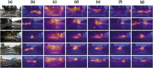
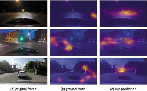
From a qualitative perspective, we chose some specific cases to visualize the prediction of the proposed model, and some better-performing models, including GBVS, LDS, FES, and MSI-Net. The comparison results are shown in Figure 2. Among these models, the GBVS model tends to predict most areas in the images as saliency, increasing the false positive rate of the salient areas, while the other four methods predict more areas in the center of the frames. Similar to the quantitative comparison, the MSI-Net and AdaFI-FCN can also make better predictions, and both are more apt to focus on the road than on other objects, such as cars, buildings, and trees. In terms of intersections and sharp turns, the proposed models predict the driver’s attention more correctly. In conclusion, the proposed model performs better in different driving scenes, and our prediction will give the driver accurate visual aids during the key driving periods.

Figure 2. The prediction maps of different models. From left to right: (a) the original frames. (b) Ground truth. (c) the GBVS model. (d) the LDS model. (e) the FES model. (f) the MSI-Net model. (g) the AdaFI-FCN model.

4.4. Ablation study

To test the performance of the proposed method, we conducted ablation studies on the sub-FCN structure and the integration of input features.

4.4.1. Ablation study on the sub-FCN structure

To demonstrate the best performance of sub-FCNs, we built up some similar model structures for sub-FCNs and then trained them with the same methods as proposed. The structure of the encoder block, the ASPP block, the decoder block, and the loss function were separately adjusted, and the introduction of these models in detail is shown in Table 5.

Table 5. The details of the comparative model structure.

Model		Description
Encoder Block	FCN _thin	Removing Layer 10–11 of sub-FCNs
	FCN _deep	Using the top 12 layers of VGG-16 in the encoder block
ASPP Block	FCN _minus_ASPP	Removing the ASPP block
Decoder Block	FCN _minus_dilation	Setting the dilation rate to 1 in the decoder block
	FCN _segmented_upsample	Using three 8 × bilinear interpolation layers for upsampling
Loss Function	FCN _minus_mean_fixation	Removing the mean fixation in the loss function

The accuracy comparison results on four metrics are shown in Table 6. Considering the four metrics comprehensively, the proposed sub-FCN structure scored better on accuracy. We tested the positive roles of the encoder block (compared with FCN_thin and FCN_deep), the ASPP block (compared with FCN_minus_ASPP), the decoder block (compared with FCN_minus_dilation and FCN_segmented_upsample), and the specially-designed loss function (compared with FCN_minus_mean_fixation). It is worth noting that, FCN_thin also showed strong prediction competitiveness if there is a need for greater prediction efficiency. However, when the prediction accuracy is given priority, the proposed framework performs better than other frameworks.

Table 6. Ablation study results on the sub-FCN structure. The AUC-Judd, CC, KL, and SIM metrics are defined in Section 4.2. The best performance in each group is marked in bold.

Model		AUC-Judd	CC	KL	SIM
Proposed model		0.971	0.767	1.046	0.579
Encoder Block	FCN_thin	0.971	0.756	1.019	0.549
	FCN_deep	0.970	0.759	1.043	0.557
ASPP Block	FCN_minus_ASPP	0.965	0.737	1.050	0.497
Decoder Block	FCN_minus_dilation	0.970	0.757	1.062	0.546
	FCN_segmented_upsample	0.970	0.763	1.063	0.565
Loss Function	FCN_minus_mean_fixation	0.970	0.756	1.105	0.570

4.4.2. Ablation study on feature integration

To demonstrate the contribution of adaptive feature integration methods, we explored the output prediction of the three sub-FCNs, and we generated the sum of these predictions without SAW. Table 7 shows the comparison result on accuracy and robustness. For three sub-FCNs, the RGB-D FCN performed better in AUC-Judd, CC, and SIM metrics, while the motion FCN listed the second. As a degraded version network with only single channel input features, the RGB-D FCN can be applied in a scenario that requires real-time prediction instead of the best accuracy performance, this result confirmed the discovery of Palazzi et al. (2019). Note that no matter whether using SAW to sum up three branches of prediction, the overall accuracy and robustness are improved, showing the advantage of feature integration. The proposed method with SAW achieved an extra improvement compared with the model without SAW.

Table 7. Ablation study result on feature integration. The AUC-Judd, CC, KL, and SIM metrics are defined in Section 4.2. $\mu$ and $c_v$ are the mean and the coefficient of variation, respectively, representing the accuracy and robustness. The best performance in each group is marked in bold.

Model	AUC-Judd		CC		KL		SIM
	$\mu$	$c_v$	$\mu$	$c_v$	$\mu$	$c_v$	$\mu$	$c_v$
RGB-D FCN	0.968	0.091	0.755	0.290	1.340	1.380	0.587	0.274
Motion FCN	0.965	0.093	0.725	0.307	1.187	1.156	0.544	0.276
Semantic FCN	0.960	0.100	0.704	0.335	1.323	1.262	0.533	0.293
Sum without SAW	0.970	0.085	0.762	0.274	1.182	1.374	0.575	0.256
Sum with SAW (proposed)	0.971	0.084	0.767	0.275	1.046	1.312	0.579	0.255

5. Discussion

5.1. The contribution of scene-adaptive weight

a) The contribution to robustness improvement

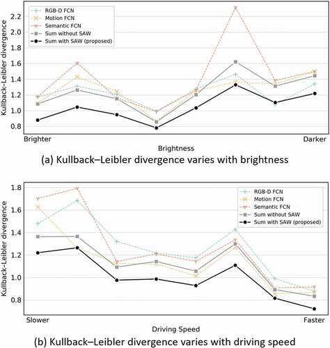
The contribution of SAW lies in the robustness improvement in the changeable driving scenes. We discussed the model’s adaptive ability to changeable scenes by two typical variables: brightness and driving speed. Figure 3 shows the KL variation with brightness and driving speed. Overall, all these compared models predicted weaker in the low brightness and in the low driving speed because of the poor quality of the input features, especially semantic segment features in these scenes. Besides, with increased driving speed, visual attention is more focused (Palazzi et al. 2019), and visual attention tends to be predicted more easily. Compared with the prediction from three sub-FCNs, the KL score of feature integration network prediction shows a more stable trend to cope with scene changes. In addition, the proposed SAW method performed better than the integration method without SAW. We concluded that the proposed SAW strategy is helpful to enhance the performance in different scenes.

Figure 3. The Kullback–Leibler divergence variation with (a) brightness and (b) driving speed. The Kullback–Leibler divergence metric was defined as Equation (6)(6) $\begin{array}{c}KL\left(Y,\hat{Y}\right)={\sum }_{i}Ylog\left(\epsilon +\frac{Y}{\epsilon +\hat{Y}}\right)\end{array}$(6) , and a lower Kullback–Leibler divergence score indicates better prediction accuracy.

b) The contribution to model interpretability

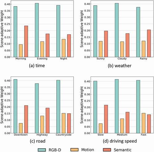
It is worth exploring the model’s dependence on different features with the scene changes by examining the SAW in an explainable way. Figure 4 shows the SAW in different scenes (times, weather, road, and driving speed). Overall, the RGB-D FCN has the largest contribution to the final prediction. This result provides powerful evidence that the importance of RGB-D information, but the task-related features still cannot be ignored. Besides, the weights of the motion FCN and the semantic FCN in different scenes show interesting variations. For different times (Figure 4(a)), the weight of the semantic FCN is greater than twice the weight of the motion FCN in the morning, while the scene becomes darker, and the weight of the motion FCN increases to the level of the semantic FCN. For different weather conditions (Figure 4(b)), the weight of the semantic FCN is higher than that of other weather conditions when raining, while the weight of the motion FCN is more stable in different weather conditions. For different roads (Figure 4(c)), the weight of the semantic FCN is higher than the motion FCN on downtown roads, and their weights are very close to each other on countryside roads. For different driving speeds (Figure 4(d)), as the driving speed increases, the weight of the motion FCN increases, while the weight of the semantic FCN decreases, showing that the dynamic cues are more valuable while high-speed driving.

Figure 4. Scene-adaptive weights in different scenes. The SAW was defined in Section 3.2.2 and was trained in the methods mentioned in Section 4.2.1.

In conclusion, we are able to explain the prediction model’s “preference” between multistream geospatial cues by the application of SAW. Besides, the SAW method can effectively decrease the effect of input feature quality differences in different scenes, especially in dark or rainy scenarios, when the feature extraction process fails to generate reliable optical flow and semantic segment features.

5.2. The balance between accuracy and efficiency

a) The combination of RGB-D feature

In this work, some necessary work was done to reduce computational cost and minimize the impact on computational efficiency. First, we combined the RGB images and the depth images to input RGB-D FCN. Instead of using two sub-FCNs to separately process the two streams of features (Eitel et al. 2015; Liang et al. 2020), our approach reduces the large memory cost and workload of building an additional sub-FCN and increases the efficiency of the network (Table 8). Besides, we found that the combination of RGB-D features also helps to improve prediction accuracy.

Table 8. The efficiency, workload, and accuracy comparison on whether or not to combine RGB-D features. The AUC-Judd, CC, KL, and SIM metrics are defined in Section 4.2.

Combining RGB-D features?	Processing Speed (frame per second, FPS)			Model workload
	Training Step 1	Training Step 2	Predicting	Parameters	FLOPs	Size
No	1.74	1.51	6.43	21.92 M	349.45 B	250.90 MB
Yes (proposed)	2.26	1.96	7.66	16.44 M	262.22 B	188.19 MB
Difference	+30.0%	+30.0%	+19.1%	−25.0%	−25.0%	−25.0%
	Prediction Accuracy
Combining RGB-D features?	AUC-Judd	CC	KL	SIM
No	0.970	0.759	1.021	0.548
Yes (proposed)	0.971	0.767	1.046	0.579
Difference	+0.10%	+1.05%	+2.45%	+5.66%

b) The removal of secondary semantic features

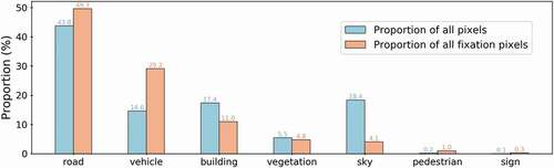
As shown in Figure 5, the road, vehicle, building, vegetation, and sky semantics occupied a large proportion of pixels (more than 99% of all the pixels). However, the road, vehicle, and building semantics occupied nearly 90% of the fixation pixels. We chose to eliminate the other four features that occupied less than 10% of all fixation pixels because the additional computational costs (especially on Layer #1 of the semantic FCN) were far outweighed by the benefits of introducing them to the model considering the low positive samples of these semantics.

Figure 5. The probability of seven semantics in all pixels and all fixation pixels. The blue bars show the proportion of each semantics’ pixels by all pixels (including fixation pixels and no-fixation pixels). The orange bars show the proportion of each semantics’ pixels by all fixation pixels.

In conclusion, for almost every deep learning classifier, it is challenging to balance accuracy and efficiency. We improved the prediction efficiency without affecting the prediction accuracy as much as possible.

5.3. Limitations and future works

The limitation of this work lies twofold. The first issue is prediction failure. As shown in Figure 6, the proposed framework failed to accurately predict the driver’s visual attention at sharp turns, intersections, or when drivers in distracted. In these particular cases, the driver’s visual attention strongly deviates from the center of the heading direction and there exist multiple locations of focus. It may inspire future work to integrate semantic information (like traffic lights and signposts) and estimated driving routes to encourage the model to make predictions in specific areas of the frame. The second issue is the salient detection at the object-level. Different from Wang et al. (2020) and Wang et al. (2021), we predicted the visual attention at the pixel-level, some further works need to be done to combine the prediction with the semantic segment image. Thus, the importance rank of each object can be computed to assist drivers in observing the outside environment.

Figure 6. Failure predictions. The proposed model failed to predict visual attention in specific scenarios, like sharp turns (top), intersections (middle) and when drivers in distracted (bottom).

In the future, there remain works on improving the prediction efficiency, and we will train the proposed framework for other driving task datasets to ensure the representation of different driver groups, such as different ages, genders, and driving experiences.

6. Conclusions

Previous studies have demonstrated the importance of geospatial information to VAP and the effects of different scene factors on the driver’s visual behavior. However, previous VAP models on drivers lacked adaptive integration of geospatial information. To solve this problem, we extracted the RGB-D, motion, and semantic features from the original RGB images. Then, we built an adaptive feature integration network with three sub-FCNs to increase the accuracy and robustness of VAP.

Our main contribution is that we use a first-proposed adaptive approach, named scene-adaptive weight, to integrate the dynamic, stereoscopic, and task-driven geospatial information related to the driving task. The quantitative and qualitative comparison results show that the proposed feature integration strategy can greatly improve the prediction performance of the model, especially in dark and rainy scenarios, besides, the proposed AdaFI-FCN achieved state-of-the-art prediction performance.

The proposed frameworks could guide novice drivers to be appropriately vigilant during the driving process. In addition, our work would use geospatial information to help drivers make decisions by highlighting key areas related to a safe drive. In addition, the proposed work could be further applied to universal geospatial scenes, such as AR-aided navigation, indoor navigation, and street-view image reading.

Data and codes availability statement

The data that support the findings of this study are openly available in figshare at: https://figshare.com/s/8b5a5390de0e08971da9 (the required training and test dataset) https://figshare.com/s/33c6915b29e34b28ff34 (the code, pretrained checkpoint, and prediction result of the framework).

Disclosure statement

No potential conflict of interest was reported by the author(s).

Additional information

Funding

This work was supported by the National Natural Science Foundation of China (NSFC) under Grant No. 42230103; and the State Key Laboratory of Geographic Information Engineering and the Key Laboratory of Surveying and Mapping Science and Geospatial Information Technology of the Ministry of Natural Resources Jointly Funded Project under Grant No. 2021-04-03.

Notes on contributors

Bowen Shi

Bowen Shi is currently a graduate student in Cartography and Geography Information System at Beijing Normal University, China. His research interests are street view image analysis and now he is focusing on spatial cognition experimental research.

Weihua Dong

Weihua Dong received the PhD degree in Cartography and Geographic Information Engineering from Wuhan University and the MSc degree in Cartography and Geographic Information Engineering from Chinese Academy of Surveying and Mapping. He is currently a Professor of Faculty of Geographical Science at Beijing Normal University and the director of the Research Center for Geospatial Cognition and Visual Analysis of Beijing Normal University. He regularly serves as an Editorial member for Cartography and Geographic Information Science, Journal of Location Based Services, and as a Guest Editor for ISPRS International Journal of Geo-Information. He is also a member of the Cognitive Working Committee of the International Cartographic Association (ICA). His research focuses on geospatial cognition and brain-like intelligent navigation. On those topics, he has authored or co-authored more than 50 articles on international journals and conferences.

Zhicheng Zhan

Zhicheng Zhan is currently a PhD candidate in Cartography and Geographical Information Science at Ghent University, Belgium. He earned his MSc degree in Cartography and Geography Information System at Beijing Normal University, China. His research interests include spatial cognition, spatial language, and indoor navigation.

References

- Alletto, S., A. Palazzi, F. Solera, S. Calderara, and R. Cucchiara. 2016. “Dr(eye)ve: A Dataset for Attention-Based Tasks with Applications to Autonomous and Assisted Driving.” Paper Presented at the IEEE Computer Society Conference on Computer Vision and Pattern Recognition Workshops (CVPRW), Las Vegas, NV, 26, 1 June-July, 54–60.
- Bak, C., A. Kocak, E. Erdem, and A. Erdem. 2018. “Spatio-Temporal Saliency Networks for Dynamic Saliency Prediction.” IEEE Transactions on Multimedia 20 (7): 1688–1698. doi:10.1109/TMM.2017.2777665.
- Bengio, Y., A. Courville, and P. Vincent. 2013. “Representation Learning: A Review and New Perspectives.” IEEE Transactions on Pattern Analysis and Machine Intelligence 35 (8): 1798–1828. doi:10.1109/tpami.2013.50.
- Borji, A., D. N. Sihite, and L. Itti. 2012. “Probabilistic Learning of Task-Specific Visual Attention.” Paper presented at the IEEE Conference on Computer Vision and Pattern Recognition (CVPR), Providence, RI, 16-21 June, 470–477.
- Bruce, N., and J. Tsotsos. 2010. “Attention Based on Information Maximization.” Journal of Vision 7 (9): 950. doi:10.1167/7.9.950.
- Bylinskii, Z., T. Judd, A. Oliva, A. Torralba, and F. Durand. 2019. “What Do Different Evaluation Metrics Tell us About Saliency Models?” IEEE Transactions on Pattern Analysis and Machine Intelligence 41 (3): 740–757. doi:10.1109/TPAMI.2018.2815601.
- Calsavara, F., F. I. K. Junior, and A. P. C. Larocca. 2021. “Effects of Fog in a Brazilian Road Segment Analyzed by a Driving Simulator for Sustainable Transport: Drivers’ Visual Profile.” Sustainability 13 (16): 9448. doi:10.3390/su13169448.
- Chen, L., Y. Zhu, G. Papandreou, F. Schroff, and H. Adam. 2018. “Encoder-Decoder with Atrous Separable Convolution for Semantic Image Segmentation.” Paper presented at the European Conference on Computer Vision (ECCV), Munich, Germany, 8-14 September, 833–851.
- Cornia, M., L. Baraldi, G. Serra, and R. Cucchiara. 2018. “Predicting Human Eye Fixations via an LSTM-Based Saliency Attentive Model.” IEEE Transactions on Image Processing 27 (10): 5142–5154. doi:10.1109/tip.2018.2851672.
- Crundall, D., C. Shenton, and G. Underwood. 2004. “Eye Movements During Intentional Car Following.” Perception 33 (8): 975–986. doi:10.1068/p5105.
- Deng, T., K. Yang, Y. Li, and H. Yan. 2016. “Where Does the Driver Look? Top-Down-Based Saliency Detection in a Traffic Driving Environment.” IEEE Transactions on Intelligent Transportation Systems 17 (7): 2051–2062. doi:10.1109/tits.2016.2535402.
- Deng, T., H. Yan, and Y. Li. 2018. “Learning to Boost Bottom-Up Fixation Prediction in Driving Environments via Random Forest.” IEEE Transactions on Intelligent Transportation Systems 19 (9): 3059–3067. doi:10.1109/tits.2017.2766216.
- Drozdzal, M., E. Vorontsov, G. Chartrand, S. Kadoury, and C. Pal. 2016. “The Importance of Skip Connections in Biomedical Image Segmentation.” Paper presented at the International Workshop on Deep Learning in Medical Image Analysis (DLMIA)/International Workshop on Large-Scale Annotation of Biomedical Data and Expert Label Synthesis (LABELS), Athens, Greece, 21 October, 179–187.
- Eitel, A., J. T. Springenberg, L. Spinello, M. Riedmiller, and W. Burgard. 2015. “Multimodal Deep Learning for Robust RGB-D Object Recognition.” Paper presented at the IEEE/RSJ International Conference on Intelligent Robots and Systems (IROS), Hamburg, Germany, 28 September 2 October, 681–687.
- Fan, L., Y. Chen, P. Wei, W. Wang, and S. Zhu. 2018. “Inferring Shared Attention in Social Scene Videos.” IEEE Conference on Computer Vision and Pattern Recognition (CVPR), Salt Lake City, UT, 18-23 June.
- Fang, S., J. Li, Y. Tian, T. Huang, and X. Chen. 2017. “Learning Discriminative Subspaces on Random Contrasts for Image Saliency Analysis.” IEEE Transactions on Neural Networks and Learning Systems 28 (5): 1095–1108. doi:10.1109/TNNLS.2016.2522440.
- Fang, Y., Z. Wang, W. Lin, and Z. Fang. 2014. “Video Saliency Incorporating Spatiotemporal Cues and Uncertainty Weighting.” IEEE Transactions on Image Processing 23 (9): 3910–3921. doi:10.1109/tip.2014.2336549.
- Fang, Y., J. Wang, M. Narwaria, P. Le Callet, and W. Lin. 2014. “Saliency Detection for Stereoscopic Images.” IEEE Transactions on Image Processing 23 (6): 2625–2636. doi:10.1109/TIP.2014.2305100.
- Fan, D., W. Wang, M. Cheng, and J. Shen. 2019. “Shifting More Attention to Video Salient Object Detection.” Paper presented at the IEEE Conference on Computer Vision and Pattern Recognition (CVPR), Long Beach, CA, 16-20 June, 8546–8556.
- Fan, L., W. Wang, S. Huang, X. Tang, and S. Zhu. 2019. “Understanding Human Gaze Communication by Spatio-Temporal Graph Reasoning.” Paper presented at the IEEE International Conference on Computer Vision (ICCV), Seoul, South Korea, 2, 27 October, November, 5723–5732.
- Farnebäck, G. 2003. “Two-Frame Motion Estimation Based on Polynomial Expansion.” Paper presented at the Scandinavian Conference on Image Analysis (SCIA), Halmstad, Sweden, 29, 2 June, July, 363–370.
- Garcia-Diaz, A., V. Leborán, X. R. Fdez-Vidal, and X. M. Pardo. 2012. “On the Relationship Between Optical Variability, Visual Saliency, and Eye Fixations: A Computational Approach.” Journal of Vision 12 (6): 17. doi:10.1167/12.6.17.
- Gershon, P., N. Ben-Asher, and D. Shinar. 2012. “Attention and Search Conspicuity of Motorcycles as a Function of Their Visual Context.” Accident Analysis & Prevention 44 (1): 97–103. doi:10.1016/j.aap.2010.12.015.
- Godard, C., O. Mac Aodha, and G. J. Brostow. 2017. “Unsupervised Monocular Depth Estimation with Left-Right Consistency.” Paper presented at the IEEE Conference on Computer Vision and Pattern Recognition (CVPR), Honolulu, HI, 21-26 July, 6602–6611.
- Guo, J., T. Ren, and J. Bei. 2016. “Salient Object Detection for RGB-D Image via Saliency Evolution.” Paper presented at the IEEE International Conference on Multimedia and Expo (ICME), Seattle, WA, 11-15 July, 1–6.
- Han, J., H. Chen, N. Liu, C. Yan, and X. Li. 2018. “CNNs-Based RGB-D Saliency Detection via Cross-View Transfer and Multiview Fusion.” IEEE Transactions on Cybernetics 48 (11): 3171–3183. doi:10.1109/TCYB.2017.2761775.
- Harel, J., C. Koch, and P. Perona. 2006. “Graph-Based Visual Saliency.” Paper presented at the International Conference on Neural Information Processing Systems (NIPS), Vancouver, British Columbia, Canada, 4–7 December, 545–552.
- Henderson, J. M. 2003. “Human Gaze Control During Real-World Scene Perception.” Trends in Cognitive Sciences 7 (11): 498–504. doi:10.1016/j.tics.2003.09.006.
- Huang, X., C. Shen, X. Boix, and Q. Zhao. 2015. “SALICON: Reducing the Semantic Gap in Saliency Prediction by Adapting Deep Neural Networks.” Paper presented at the IEEE International Conference on Computer Vision (ICCV), Santiago, Chile, 7-13 December, 262–270.
- Huang, J., X. Zhang, Q. Xin, Y. Sun, and P. Zhang. 2019. “Automatic Building Extraction from High-Resolution Aerial Images and LiDar Data Using Gated Residual Refinement Network.” ISPRS Journal of Photogrammetry and Remote Sensing 151: 91–105. doi:10.1016/j.isprsjprs.2019.02.019.
- Itti, L., C. Koch, and E. Niebur. 1998. “A Model of Saliency-Based Visual Attention for Rapid Scene Analysis.” IEEE Transactions on Pattern Analysis and Machine Intelligence 20 (11): 1254–1259. doi:10.1109/34.730558.
- Jiang, M., S. S. Huang, J. Y. Duan, and Q. Zhao. 2015. “SALICON: Saliency in Context.” Paper presented at the IEEE Conference on Computer Vision and Pattern Recognition (CVPR), Boston, MA, 7-12 June, 1072–1080.
- Jiang, L., M. Xu, T. Liu, M. Qiao, and Z. Wang. 2018. “DeepVs: A Deep Learning Based Video Saliency Prediction Approach.” Paper presented at the European Conference on Computer Vision (ECCV), Munich, Germany, 8-14 September, 625–642.
- Jo, D., S. Lee, and Y. Lee. 2014. “The Effect of Driving Speed on Driver’s Visual Attention: Experimental Investigation.” Paper presented at the International Conference on Engineering Psychology and Cognitive Ergonomics (EPCE), Heraklion, Crete, Greece, 22-27 June, 174–182.
- Judd, T., F. Durand, and A. Torralba. 2012. “A Benchmark of Computational Models of Saliency to Predict Human Fixations.” MIT Technical Report.
- Judd, T., K. Ehinger, F. Durand, and A. Torralba. 2009. “Learning to Predict Where Humans Look.” Paper presented at the IEEE International Conference on Computer Vision (ICCV), Kyoto, Japan, 29, 2 September, October, 2106–2113.
- Kang, B., and Y. Lee. 2020. “High-Resolution Neural Network for Driver Visual Attention Prediction.” Sensors 20 (7): 2030. doi:10.3390/s20072030.
- Koch, C., and S. Ullman. 1985. “Shifts in Selective Visual Attention: Towards the Underlying Neural Circuitry.” Human Neurobiology 4 (4): 219–227.
- Konstantopoulos, P., P. Chapman, and D. Crundall. 2010. “Driver’s Visual Attention as a Function of Driving Experience and Visibility. Using a Driving Simulator to Explore Drivers’ Eye Movements in Day, Night and Rain Driving.” Accident Analysis & Prevention 42 (3): 827–834. doi:10.1016/j.aap.2009.09.022.
- Krizhevsky, A., I. Sutskever, and G. E. Hinton. 2012. “ImageNet Classification with Deep Convolutional Neural Networks.” Paper presented at the International Conference on Neural Information Processing Systems (NIPS), Lake Tahoe, NV, 3-8 December, 1097–1105.
- Kroner, A., M. Senden, K. Driessens, and R. Goebel. 2020. “Contextual Encoder-Decoder Network for Visual Saliency Prediction.” Neural Networks 129: 261–270. doi:10.1016/j.neunet.2020.05.004.
- Kruthiventi, S. S. S., K. Ayush, and R. V. Babu. 2017. “DeepFix: A Fully Convolutional Neural Network for Predicting Human Eye Fixations.” IEEE Transactions on Image Processing 26 (9): 4446–4456. doi:10.1109/tip.2017.2710620.
- Kwak, S., B. Ko, and H. Byun. 2007. “Salient Human Detection for Robot Vision.” Pattern Analysis and Applications 10 (4): 291–299. doi:10.1007/s10044-007-0068-8.
- Lai, Q., W. Wang, H. Sun, and J. Shen. 2020. “Video Saliency Prediction Using Spatiotemporal Residual Attentive Networks.” IEEE Transactions on Image Processing 29: 1113–1126. doi:10.1109/tip.2019.2936112.
- Lang, C., T. V. Nguyen, H. Katti, K. Yadati, M. Kankanhalli, and S. Yan. 2012. “Depth Matters: Influence of Depth Cues on Visual Saliency.” Paper presented at the European Conference on Computer Vision (ECCV), Florence, Italy, 7-13 October, 101–115.
- Lateef, F., M. Kas, and Y. Ruichek. 2022. “Saliency Heat-Map as Visual Attention for Autonomous Driving Using Generative Adversarial Network (GAN).” IEEE Transactions on Intelligent Transportation Systems 23 (6): 5360–5373. doi:10.1109/TITS.2021.3053178.
- Lecun, Y., L. Bottou, Y. Bengio, and P. Haffner. 1998. “Gradient-Based Learning Applied to Document Recognition.” Proceedings of the IEEE 86 (11): 2278–2324. doi:10.1109/5.726791.
- Leifman, G., D. Rudoy, T. Swedish, E. Bayro-Corrochano, and R. Raskar. 2017. “Learning Gaze Transitions from Depth to Improve Video Saliency Estimation.” Paper presented at the IEEE International Conference on Computer Vision (ICCV), Venice, Italy, 22-29 October, 1698–1707.
- Liang, F., L. Duan, W. Ma, Y. Qiao, Z. Cai, J. Miao, and Q. Ye. 2020. “CoCnn: RGB-D Deep Fusion for Stereoscopic Salient Object Detection.” Pattern Recognition 104 (9): 107329. doi:10.1016/j.patcog.2020.107329.
- Liao, H., W. Dong, H. Huang, G. Gartner, and H. Liu. 2019. “Inferring User Tasks in Pedestrian Navigation from Eye Movement Data in Real-World Environments.” International Journal of Geographical Information Science 33 (4): 739–763. doi:10.1080/13658816.2018.1482554.
- Lin, Y., Y. Tang, B. Fang, Z. Shang, Y. Huang, and S. Wang. 2013. “A Visual-Attention Model Using Earth Mover’s Distance-Based Saliency Measurement and Nonlinear Feature Combination.” IEEE Transactions on Pattern Analysis and Machine Intelligence 35 (2): 314–328. doi:10.1109/TPAMI.2012.119.
- Liu, B., L. Sun, and J. Rong. 2011. “Driver’s Visual Cognition Behaviors of Traffic Signs Based on Eye Movement Parameters.” Journal of Transportation Systems Engineering and Information Technology 11 (4): 22–27. doi:10.1016/S1570-6672(10)60129-8.
- Miura, T., K. Shinohara, T. Kimura, and K. Ishimatsu. 2005. “Characteristics of Visual Attention and the Safety.” Systems and Human Science for Safety, Security and Dependability 63–73.
- Muddamsetty, S., D. Sidibé, A. Treméau, and F. Meriaudeau. 2013. “A Performance Evaluation of Fusion Techniques for Spatio-Temporal Saliency Detection in Dynamic Scenes.” Paper presented at the IEEE International Conference on Image Processing (ICIP), Melbourne, Australia, 15-18 September, 3924–3928.
- Ning, Z., J. Luo, Y. Li, S. Han, Q. Feng, Y. Xu, W. Chen, T. Chen, and Y. Zhang. 2019. “Pattern Classification for Gastrointestinal Stromal Tumors by Integration of Radiomics and Deep Convolutional Features.” IEEE Journal of Biomedical and Health Informatics 23 (3): 1181–1191. doi:10.1109/jbhi.2018.2841992.
- Ogasawara, K., T. Miyazaki, Y. Sugaya, and S. Omachi. 2020. “Object-Based Video Coding by Visual Saliency and Temporal Correlation.” IEEE Transactions on Emerging Topics in Computing 8 (1): 168–178. doi:10.1109/TETC.2017.2695640.
- Oliva, A., A. Torralba, M. S. Castelhano, and J. M. Henderson. 2003. “Top-Down Control of Visual Attention in Object Detection.” Paper presented at the IEEE International Conference on Image Processing (ICIP), Barcelona, Spain, 14-17 September, 1–253.
- Palazzi, A., D. Abati, S. Calderara, F. Solera, and R. Cucchiara. 2019. “Predicting the Driver’s Focus of Attention: The Dr(eye)ve Project.” IEEE Transactions on Pattern Analysis and Machine Intelligence 41 (7): 1720–1733. doi:10.1109/TPAMI.2018.2845370.
- Pan, J., C. Canton-Ferrer, K. McGuinness, N. O’Connor, J. Torres, E. Sayrol, and X. Giro-i-Nieto. 2017. “SalGan: Visual Saliency Prediction with Generative Adversarial Networks.” ArXiv abs/1701.01081. doi:10.48550/arXiv.1701.01081.
- Richardson, E. D., and R. A. Marottoli. 2003. “Visual Attention and Driving Behaviors Among Community-Living Older Persons.” The Journals of Gerontology: Series A 58 (9): 832–836. doi:10.1093/gerona/58.9.M832.
- Rogalska, A., and P. Napieralski. 2018. “The Visual Attention Saliency Map for Movie Retrospection.” Open Physics 16 (1): 188–192. doi:10.1515/phys-2018-0027.
- Ronneberger, O., P. Fischer, and T. Brox. 2015. “U-Net: Convolutional Networks for Biomedical Image Segmentation.” Paper presented at the International Conference on Medical Image Computing and Computer-Assisted Intervention (MICCAI), Munich, Germany, 5-9 October, 234–241.
- Rueopas, W., S. Leelhapantu, and T. H. Chalidabhongse. 2016. “A Corner-Based Saliency Model.” Paper presented at the International Joint Conference on Computer Science and Software Engineering (JCSSE), Khon Kaen, Thailand, 13-15 July, 1–6.
- Simonyan, K., and A. Zisserman. 2015. “Very Deep Convolutional Networks for Large-Scale Image Recognition.” ArXiv abs/1409.1556. doi:10.48550/arXiv.1409.1556.
- Song, H., Z. Liu, H. Du, G. Sun, O. Le Meur, and T. Ren. 2017. “Depth-Aware Salient Object Detection and Segmentation via Multiscale Discriminative Saliency Fusion and Bootstrap Learning.” IEEE Transactions on Image Processing 26 (9): 4204–4216. doi:10.1109/TIP.2017.2711277.
- Tavakoli, H. R., E. Rahtu, and J. Heikkilä. 2011. “Fast and Efficient Saliency Detection Using Sparse Sampling and Kernel Density Estimation.” Paper presented at the Scandinavian Conference on Image Analysis (SCIA), Ystad Saltsjöbad, Sweden, 23-27 May, 666–675.
- Tawari, A., and B. Kang. 2017. “A Computational Framework for Driver’s Visual Attention Using a Fully Convolutional Architecture.” Paper presented at the IEEE Intelligent Vehicles Symposium (IV), Redondo Beach, CA, 11-14 June, 887–894.
- Treisman, A. M., and G. Gelade. 1980. “A Feature-Integration Theory of Attention.” Cognitive Psychology 12 (1): 97–136. doi:10.1016/0010-0285(80)90005-5.
- Trick, L. M., R. Toxopeus, and D. Wilson. 2010. “The Effects of Visibility Conditions, Traffic Density, and Navigational Challenge on Speed Compensation and Driving Performance in Older Adults.” Accident Analysis & Prevention 42 (6): 1661–1671. doi:10.1016/j.aap.2010.04.005.
- Wang, P., P. Chen, Y. Yuan, D. Liu, Z. Huang, X. Hou, and G. Cottrell. 2018. “Understanding Convolution for Semantic Segmentation.” Paper presented at the IEEE Winter Conference on Applications of Computer Vision (WACV), Lake Tahoe, NV, 11-15 March, 1451–1460.
- Wang, J., H. Jiang, Z. Yuan, M. Cheng, X. Hu, and N. Zheng. 2017. “Salient Object Detection: A Discriminative Regional Feature Integration Approach.” International Journal of Computer Vision 123 (2): 251–268. doi:10.1007/s11263-016-0977-3.
- Wang, Y., B. Liang, M. Ding, and J. Li. 2019. “Dense Semantic Labeling with Atrous Spatial Pyramid Pooling and Decoder for High-Resolution Remote Sensing Imagery.” Remote Sensing 11 (1): 20. doi:10.3390/rs11010020.
- Wang, W., and J. Shen. 2018. “Deep Visual Attention Prediction.” IEEE Transactions on Image Processing 27 (5): 2368–2378. doi:10.1109/tip.2017.2787612.
- Wang, W., J. Shen, X. Dong, A. Borji, and R. Yang. 2020. “Inferring Salient Objects from Human Fixations.” IEEE Transactions on Pattern Analysis and Machine Intelligence 42 (8): 1913–1927. doi:10.1109/tpami.2019.2905607.
- Wang, W., J. Shen, F. Guo, M. Cheng, and A. Borji. 2018. “Revisiting Video Saliency: A Large-Scale Benchmark and a New Model.” Paper presented at the IEEE Conference on Computer Vision and Pattern Recognition (CVPR), Salt Lake City, UT, 18-23 June, 4894–4903.
- Wang, W., J. Shen, and Y. Jia. 2019. “Review of Visual Attention Detection.” Journal of Software 30 (2): 416–439.
- Wang, W., J. Shen, X. Lu, S. C. H. Hoi, and H. Ling. 2021. “Paying Attention to Video Object Pattern Understanding.” IEEE Transactions on Pattern Analysis and Machine Intelligence 43 (7): 2413–2428. doi:10.1109/tpami.2020.2966453.
- Wang, A., and M. Wang. 2017. “RGB-D Salient Object Detection via Minimum Barrier Distance Transform and Saliency Fusion.” IEEE Signal Processing Letters 24 (5): 663–667. doi:10.1109/lsp.2017.2688136.
- Wang, Z., C. Zou, and W. Cai. 2020. “Small Sample Classification of Hyperspectral Remote Sensing Images Based on Sequential Joint Deeping Learning Model.” IEEE Access 8: 71353–71363. doi:10.1109/access.2020.2986267.
- Xue, H., M. Sun, and Y. Liang. 2022. “ECANet: Explicit Cyclic Attention-Based Network for Video Saliency Prediction.” Neurocomputing 468: 233–244. doi:10.1016/j.neucom.2021.10.024.
- Zhan, Z., and W. Dong. 2021. “A Multi-Feature Approach for Modeling Visual Saliency of Dynamic Scene for Intelligent Driving.” Acta Geodaetica et Cartographica Sinica 50 (11): 1500–1511. doi:10.11947/j.AGCS.2021.20210266.
- Zhang, L., M. H. Tong, T. Marks, H. Shan, and G. Cottrell. 2008. “SUN: A Bayesian Framework for Saliency Using Natural Statistics.” Journal of Vision 8 (7): 1–20. doi:10.1167/8.7.32.
- Zhao, S., G. Han, Q. Zhao, and P. Wei. 2020. “Prediction of Driver’s Attention Points Based on Attention Model.” Applied Sciences 10 (3): 1083. doi:10.3390/app10031083.
- Zhao, C., and C. Liu. 2010. “Sparse Embedding Feature Combination Strategy for Saliency-Based Visual Attention System.” Journal of Computational Information Systems 6 (9): 2831–2838.
- Zhou, X., Z. Liu, C. Gong, and W. Liu. 2018. “Improving Video Saliency Detection via Localized Estimation and Spatiotemporal Refinement.” IEEE Transactions on Multimedia 20 (11): 2993–3007. doi:10.1109/tmm.2018.2829605.