Modelling future spatial distribution of peanut crops in Australia under climate change scenarios

ABSTRACT

One of the major impacts of climate change in the agricultural sector relates to changes in the suitability of areas that are used for planting crops. Since peanut (Arachis hypogaea L.) is one of the most important sources of protein, an assessment of the potential shifts in peanut crop planting areas is critical. In this study, we evaluated the effects of climate change on the potential distribution of peanut crops in Australia. The current and potential future distributions of peanut crops were modeled using Species Distribution Models (SDMs) of CLIMatic indEX (CLIMEX). The future potential peanut crop distributions in Australia for 2030, 2050, 2070, and 2100 were modeled by employing CSIRO-Mk3.0 and MIROC-H Global Climate Models (GCMs) under SRES A2 climate change scenarios from CliMond 10’ database. The results indicated an increase in unsuitable areas for peanut cultivation in Australia throughout the projected years for the two GCMs. The CSIRO-Mk3.0 projection of unsuitable areas in 2100 was higher (i.e. 76% of the Australian continent) than the MIROC-H projection (i.e. 48% of the Australian continent). It was found that the projected increase in dry stress in the future could cause limitations in areas that are currently suitable for peanut crop cultivation. Looking into the future suitability of existing peanut cultivation areas, both GCMs agreed that some areas will become unsuitable, while they disagreed with the suitability of other areas. However, they agreed on the important point that only a small number of existing peanut cultivation areas would still be suitable in the future. Using CLIMEX, the present study has confirmed the effects of climate change on the shifts in areas suitable for peanut cultivation in the future, and thus may provide valuable information relevant to the long-term planning of peanut cultivation in Australia.

KEYWORDS:

• CLIMEX
• cropping areas
• climate change
• peanut
• Australia
• GCMs

1. Introduction

Climate change is ongoing and inevitable. As weather and climate have a significant influence on agricultural production (Zhao et al. 2017; Nguyen-Huy et al. 2018), future climate change and climate variability place agriculture as a susceptible sector (Anwar et al. 2013). Research indicates that the increase in anthropogenic gas emissions is the dominant cause of climate change (IPCC 2014). The increase in emissions leads to alterations in mean temperature, climate variability, and increasing extreme weather events, such as very high or very low temperatures, drought, heavy rainfall, flooding, and tropical storms (Gornall et al. 2010; Waterfield 2018). From 1850–1900 to 2010–2019, global surface temperature has risen between 0.8°C and 1.3°C (Masson-Delmotte et al. 2021). It was recorded that the temperature of the last four decades has consecutively increased compared to any decade since 1850 (Masson-Delmotte et al. 2021). If there will be no changes in the current emission rates, it is projected that between 2030 and 2052, the temperature will increase by 1.5°C (Waterfield 2018). Therefore, the Paris Agreement was introduced in 2015 with the aim to limit the increase in global temperature to 2°C by 2100 and to pursue effort in limiting the temperature increase to 1.5°C (Fawzy et al. 2020). This long-term global goal was reaffirmed at the UN Climate Change Conference UK 2021 or COP26 (UNFCCC 2021).

Australia’s climate is influenced by El Nino – Southern Oscillation (ENSO), the Indian Ocean Dipole (IOD), the Madden-Julian Oscillation (MJO), and the Southern Annular Mode (SAM) (King et al. 2014; CSIRO, and BoM 2015), all of which lead to Australia having one of the most variable climates in the world (Potgieter et al. 2013; DERM 2010). Over the last 50 years, Australia has become hotter with substantial changes in the geographic distribution of rainfall (DERM 2010). The country has experienced a mean temperature increase of 1.4°C since 1910, with a rapid increase in extreme heat events and a decline in rainfall in southern and eastern regions (CSIRO, and BoM 2020; Canadell et al. 2021). As a result of the variability, climate change will continue to significantly influence Australia's agricultural sector.

The climate in the future will be different to the climate at present and in the past (DERM 2010; Steffen et al. 2012). Global Climate Models (GCMs) are among the best instruments for projecting climate change. These are developed using mathematical representations of the climate systems, based on the laws of physics, including conservation of mass, energy, and momentum (CSIRO, and BoM 2015; Suppiah et al. 2007). The projections are built by accounting for the main natural and anthropogenic radiative forces, such as greenhouse gases, aerosols, land use, and solar output (Tang et al. 2019). It is predicted that under all emissions scenarios in the climate projections, further temperature increase will occur until mid-century (Masson-Delmotte et al. 2021).

Because of the impacts of climate change, agricultural industries are exposed to a number of risks like heat stress, drought, water availability, waterlogging, salinity, the occurrence of pests and diseases, reduction in production, and unsuitability of current planting areas (Steffen et al. 2012; Gornall et al. 2010). Major factors determining the geographic boundary in planting crops include soil quality, availability of nutrients, and climate (Anwar et al. 2013; Ujoh, Igbawua, and Ogidi Paul 2019). In particular, geographical distribution and growth of plant species will be significantly affected by climate change (Scheffers et al. 2016), although the scale will depend on the species type (annuals or perennials) and their growth patterns (agricultural crops or natural vegetation) (Coakley, Scherm, and Chakraborty 1999). Unfortunately, in most landscapes, plant species are unable to cope with the projected climate change, which results in a natural shift in their geographical range (IPCC 2014). If the climate changes as projected, there will be shifts in crop areas planted and the occurrence of pests and diseases, which could lead to economic impacts from crop loss (Chakraborty, Tiedemann, and Teng 2000). Therefore, studies on the spatio-temporal dynamics of cropland and cropping pattern changes are crucial to understand the underlying factors and the functional effects of the agricultural landscape (Rahman and Saha 2009).

Peanut (Arachis hypogaea L.) is one of the most important sources of protein and has 26% more protein than eggs, dairy products, meat, or fish (DPIF 2007). Peanut crops require relatively warm conditions, an abundance of sunshine, 500–600 mm well-distributed rainfall, and stored soil water to harvest a high-yielding crop (Halder et al. 2020). Peanut crops originated in South America and have adapted without problems to warmer regions of Australia (DPIF 2007). Queensland is the main peanut cropping area in Australia, producing more than 90% of Australia’s peanuts (GRDC 2014). Originally, peanut crops were grown in the Burnett and the Atherton Tableland regions in Queensland, but in 1990s, the cropping areas expanded into other Queensland areas, namely Bundaberg, Mackay, Emerald, and southern Queensland (Crosthwaite 1994; DPIF 2007). Currently, the peanut planting areas further expand into Katherine in the Northern Territory and other Queensland areas, i.e. Texas, Inglewood, St. George, Childers, Chinchilla, and Georgetown (Chauhan et al. 2013).

Like other crops, peanut crops can also be affected by climate change. In Australia, peanuts are traditionally cultivated in dryland conditions (Chauhan et al. 2013). Unfortunately, since Australia’s climate is highly variable (Nguyen-Huy et al. 2020) due to the impact of El Nino-Southern Oscillation (ENSO) (Nicholls, Drosdowsky, and Lavery 1997), unfavorable weather conditions, for instance drought and excessive rainfall, can easily affect peanut production in the country (Meinke, Stone, and Hammer 1996). As climate holds an important role in determining crop planting suitability (Anwar et al. 2013), it is projected that the future geographic distribution of peanut crops will be affected.

Shifting geographic distribution of crops due to climate change can be mapped using modeling techniques such as Species Distribution Models (SDMs). A fundamental approach of SDMs is that climate ultimately limits the distribution of species (Beaumont, Hughes, and Pitman 2008). These models establish the relationship between known species distribution data and environmental variables and/or spatial characteristics of those locations to determine appropriate environmental conditions for a species to survive (Joshi et al. 2011; Elith and Leathwick 2009). The resulting data can then be used to predict species potential distribution under a particular climate change scenario (Heikkinen et al. 2006). This condition makes SDMs a valuable tool in the study of invasive species (Joshi et al. 2011). Some examples of SDMs are MaxEnt, ANUCLIM/BIOCLIM, CLIMATE, CLIMATE ENVELOPE, DOMAIN, GARP, HABITAT, and CLIMatic indEX(CLIMEX) (Kriticos and Randall 2001; Gogol-Prokurat 2011; Liu et al. 2015). In statistical modeling of species distribution, three components are required, namely ecological model (ecological knowledge and theory), data model (the collection and measurement/estimation of data), and statistical model (statistical method, error function, and significance tests) (Austin 2002).

CLIMEX (Sutherst and Maywald 1985) is a simplified dynamic computer model that deduces species’ or other biological entities’ responses to climate, based on their geographical distribution and their seasonal growth and mortality patterns in different areas (Kriticos et al. 2015). It is based on the key assumption that if it is known where a species lives, it will be possible to deduce tolerant climatic conditions for the species, an assumption also used by other models. However, while other correlative statistical models try to characterize species’ occupied environments, CLIMEX attempts to mimic mechanisms that limit the geographical distribution of the species, determine species’ seasonal phenology, and to some extent determine species’ relative abundance (Kriticos et al. 2015). CLIMEX also facilitates the need to contain dynamic elements, which is often missing in correlative models, by depicting the response of species to a set of climatic variables at daily or temporal scales (Kriticos et al. 2015). The model has been widely used to predict future geographic distributions of several crops, such as the common bean (Ramirez-Cabral, Kumar, and Taylor 2016), wheat and cotton (Shabani and Kotey 2015), oil palms (Paterson et al. 2015), tomato (Silva et al. 2017), and date palms (Shabani, Kumar, and Taylor 2014, 2015). However, to the best of our knowledge, studies regarding the projected suitable areas for peanut cultivation in the future have not been carried out in any part of the world, including Australia.

Recently, Australia’s climate has been becoming warmer and is projected to continue in the future, which increases the possibility of extremely hot summers (DERM 2010; King, Karoly, and Henley 2017). Consequently, some regions could turn out to be more suitable for future peanut planting, while others could turn out to be less favorable. Moreover, the analysis of land suitability for crops is a key factor for irrigation development and crop productivity improvement to ensure food security and stable expansion of agricultural production (Al-Hanbali et al. 2021; Sarkar, Ghosh, and Banik 2014). Therefore, it is important to identify and map which areas will be favorable for peanut production in the future, and which areas will be adversely affected by climate change impacts. Performing these tasks will provide useful knowledge in anticipating climate change effects in this commodity. The primary aim of this study was to evaluate the effects of climate change on the future geographic distribution of peanut crops in Australia. The following are the specific objectives: 1) to develop CLIMEX model parameters on geographic distribution of peanut crops by using current crop distribution and climate data and 2) to project and analyze the potential future geographic distribution of peanut crops in Australia under two different climate models.

2. Materials and methods

2.1. Study area

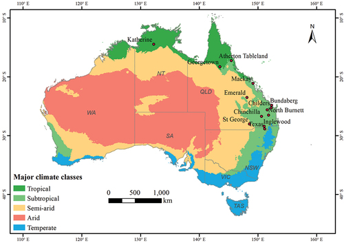
This study covered the entire Australian continent (Figure 1), with a total area of 7.692 million km² (Geoscience Australia 2018). Australia has a variety of climates comprising five major climate groups, i.e. tropical, subtropical, semi-arid, arid, and temperate (Kriticos et al. 2012). This climate classification is based on the Koppen-Geiger classification system, which was developed by applying the rules of Kriticos et al. (2012) to the 5’resolution WorldClim global climatology (Hijmans et al. 2005). Agricultural lands in Australia are located in the eastern parts of Queensland and New South Wales, the majority of Victoria, the southern part of South Australia, and the south-western part of Western Australia (ABARES 2019). These agricultural lands are dominated by subtropical, semi-arid, and temperate climates. Summer crops planted in Australia are sorghums, cottons, rice paddies, corns, mung beans, peanuts, soybeans, and sunflowers, while winter crops planted are wheat, barleys, canola, chickpeas, faba beans, field peas, lentils, lupine, oats, safflower, and triticale (ABARES 2016).

Figure 1. Map of the study area (Australia) with the locations (town and cities) of peanut cropping areas throughout different climate zones. Adapted from Kriticos et al. (2012).

2.2. Research flowchart

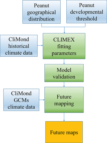
The entire workflow employed in this study is presented in Figure 2.

Figure 2. Flow chart of data and key processing tasks employed in the study.

2.3. Data acquisition

2.3.1. Peanut crop geographic distribution

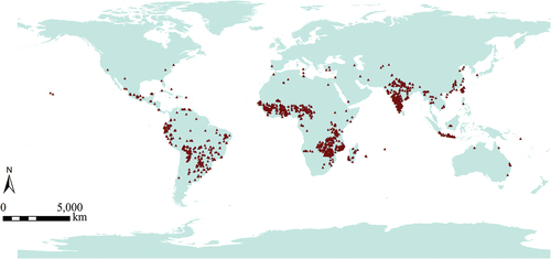
Data representing the current distribution of peanut (Arachis hypogaea L.) (Figure 3) were obtained from the Global Biodiversity Information Facility (GBIF 2017) and the Atlas of Living Australia (ALA 2017). A total of 9,011 records were obtained from these databases. However, only 1,912 records were used in this study, since the other 7,099 records were identified as records without geographic coordinates, preserved specimens, duplicate records, and data outliers. During the CLIMEX model parameter development, these geographic distribution records were divided into two: one area was used for parameter fitting, while the other area was used for model validation. This division is important to ensure data independence of model validation, thus affirming the reliability of the model.

Figure 3. The current data site distribution of peanut crops taken from GBIF (2017) and ALA (2017). Red triangles represent the distribution data.

2.3.2. Climate data and climate change models and scenarios

The CliMond gridded climate data at 10’ resolution (Kriticos et al. 2012) was employed to model the geographical distribution of peanut crops. The climate variables used to run the CLIMEX model are average maximum monthly temperature (T_max), average minimum monthly temperature (T_min), average monthly precipitation (P_total) and Relative Humidity recorded at 9:00 am (RH_09:00) and 3:00 pm (RH_15:00) (Kriticos et al. 2012). Historical climate data of these five climate variables for a period of 1950–2000 (centered at 1975) were retrieved from the CliMond database to develop peanut CLIMEX parameters. The same climate variables were also used to model future peanut distribution in Australia by employing GCMs and the climate change scenarios.

Two GCMs, i.e. CSIRO-Mk3.0 (developed by CSIRO, Australia) and MIROC-H (developed by the Center for Climate Research, Japan) were used in this study and downloaded from the CliMond database. The choice of these GCMs was based on three criteria (Kriticos et al. 2012): 1) their availability of monthly averages of minimum and maximum daily temperature, precipitation, mean sea-level pressure, and specific humidity; 2) their relatively small horizontal grid spacing; and 3) their superior performance relative to other GCMs. The SRES (Special Report on Emissions Scenarios) A2 family (Nakicenovic et al. 2000) was used as emission scenarios for both GCMs. The “A” family of SRES emission scenarios is the most extreme SRES scenario family; it was chosen in this study based on its consistency with the emission of carbon dioxide since 2000 (Manning et al. 2010). The A2 emission scenario family depicts the world as very heterogeneous with high population growth, but slow economic growth, largely due to slow changes in technology (Bernstein et al. 2008). This scenario family’s theme is self-reliance and local identities preservation, which leads to regional orientation of economic development (Nakicenovic et al. 2000).

2.4. Species distribution model (SDMs)

2.4.1. CLIMEX model

CLIMEX is a dynamic model based on a mechanistic (process-oriented) approach of species population processes. This enables the determination of a species’ relative abundance, potential geographic distribution, and seasonal variations based on climate-related processes (Kriticos et al. 2015). There are three options for running the model: compare locations, compare years, and compare locations/years (Kriticos et al. 2015), and this study has employed the compare locations option. The model can utilize the minimum field data by extracting the maximum information of species’ responses to climate (Sutherst 2003). It works on the assumption that most species experienced both favorable season(s) for population growth, which is known as the growth season and unfavorable season(s) for population growth, which is known as the survival or stress season (Sutherst 2003; Kriticos et al. 2015).

The CLIMEX model develops a Growth Index (GI_A) to describe the potential species’ growth during favorable season(s), and a Stress Index (SI) to describe the survival ability of species during unfavorable season(s). The philosophy of the model is that a range of climatic parameters defined by Growth Indices (i.e. Temperature Index (TI_W) and Moisture Index (MI_W)) will determine species’ population growth. Values outside these ranges will stimulate stress and lead to a negative population growth, which is described by Stress Indices: Cold Stress (CS), Heat Stress (HS), Dry Stress (DS), and Wet Stress (WS). Growth and Stress Indices define species’ responses to temperature, soil moisture, and if applicable, light. The CLIMEX program calculated these indices every week, then combined them into an annual value. The purpose of the model is to combine the GI and SI indices into an Ecoclimatic Index (EI) value, which describes the climatic favorability of a location for a species’ permanent occupation (Kriticos et al. 2015; Sutherst and Maywald 1985). The EI can be calculated as follows:

(1) $\mathrm{E}\mathrm{I}=\mathrm{G}{\mathrm{I}}_{\mathrm{A}}\times \mathrm{S}\mathrm{I}$(1)

where:

(2) $\mathrm{G}{\mathrm{I}}_{\mathrm{A}},\mathrm{t}\mathrm{h}\mathrm{e}\mathrm{a}\mathrm{n}\mathrm{n}\mathrm{u}\mathrm{a}\mathrm{l}\mathrm{G}\mathrm{r}\mathrm{o}\mathrm{w}\mathrm{t}\mathrm{h}\mathrm{I}\mathrm{n}\mathrm{d}\mathrm{e}\mathrm{x},=100{\sum }_{i=1}^{52}\mathrm{G}{\mathrm{I}}_{\mathrm{w}}/52$(2)

(3) $\mathrm{G}{\mathrm{I}}_{\mathrm{W},}\mathrm{t}\mathrm{h}\mathrm{e}\mathrm{w}\mathrm{e}\mathrm{e}\mathrm{k}\mathrm{l}\mathrm{y}\mathrm{G}\mathrm{r}\mathrm{o}\mathrm{w}\mathrm{t}\mathrm{h}\mathrm{I}\mathrm{n}\mathrm{d}\mathrm{e}\mathrm{x}=\mathrm{T}{\mathrm{I}}_{\mathrm{W}}\times \mathrm{M}{\mathrm{I}}_{\mathrm{W}}$(3)

TI_W is weekly Temperature Index and MI_W is weekly Moisture Index

(4) $\begin{array}{cc}& \hspace{0.17em}\mathrm{S}\mathrm{I},\mathrm{t}\mathrm{h}\mathrm{e}\mathrm{a}\mathrm{n}\mathrm{n}\mathrm{u}\mathrm{a}\mathrm{l}\mathrm{S}\mathrm{t}\mathrm{r}\mathrm{e}\mathrm{s}\mathrm{s}\mathrm{I}\mathrm{n}\mathrm{d}\mathrm{e}\mathrm{x},\\ & =\left[\left(1-\frac{\mathrm{C}\mathrm{S}}{100}\right)\times \left(1-\frac{\mathrm{D}\mathrm{S}}{100}\right)\times \left(1-\frac{\mathrm{H}\mathrm{S}}{100}\right)\times \left(1-\frac{\mathrm{W}\mathrm{S}}{100}\right)\right]\end{array}$(4)

CS, DS, HS, WS, respectively are the annual cold, dry, heat, and wet stress indices.

The Ecoclimatic Index (EI) value ranges from 1 to 100 which denotes unsuitable to optimal conditions for a species to survive in one location. If the climate of a location is ideal for a species to persist throughout the year, the EI value will be 100. However, this rarely occurs since GI seldom reaches its maximum value (Kriticos and Leriche 2010; Kriticos et al. 2015). In areas with distinct wet and dry seasons, it would be expected that the maximum EI value would be around 50 (Kriticos et al. 2015; Sutherst 2003). It has been found that EI values of more than 20 have been adequate to support substantial population densities, while EI values of less than 10 indicate that the location is likely to experience large annual climate fluctuation and is therefore marginal for species’ permanent occupation (Sutherst 2003). The EI classification used in this study was defined as follows: unsuitable (EI = 0), marginal (0 < EI < 10), suitable (10< EI  < 20), and optimal (EI > 20).

2.4.2. Fitting CLIMEX parameters

The most challenging task in CLIMEX modeling is fitting species’ CLIMEX parameters. It requires an understanding of global geography and climatic patterns and the sensitivity of Stress and Growth indices (Kriticos et al. 2015). The underlying philosophy is that Stress Indices limit the geographical distribution of the species, while Growth Indices indicate the seasonal population growth (Ramirez-Cabral, Kumar, and Taylor 2016; Kriticos et al. 2015). In addition, the resulting parameters should be biologically reasonable, based on theoretical and practical species’ knowledge from experimental domains (Kriticos et al. 2015).

As with other CLIMEX studies (Ramirez-Cabral, Kumar, and Taylor 2016; Taylor et al. 2012), this study also used native and exotic distribution data with a heterogeneous environment to fit peanut CLIMEX parameters. A heterogeneous environment with variable climates is recommended in fitting CLIMEX parameters (Kriticos et al. 2015; Sutherst 2003), since it facilitates the required range of possible temperature and moisture values for species’ permanent occupations (Sutherst 2003). Furthermore, in fitting the parameters, Sutherst (2003) and Kriticos and Leriche (2010) have suggested the use of both native and exotic (agricultural worldwide) distribution data of the species. After being released from the effects of natural enemies, a species might occupy exotic distribution areas, which have totally different climate ranges from the native distribution areas. Therefore, the inclusion of these climate ranges will enhance the model’s ability to approximate the species’ potential distribution (Kriticos et al. 2015; Kriticos and Leriche 2010; Sutherst 2003).

In this study, peanut geographical distribution data, which provides general pictures of peanut climatic preferences, was used as a guideline in fitting CLIMEX parameters. Comparing the peanut distribution data with the available CLIMEX template, this study chose the CLIMEX wet tropical template, which showed the best fit with overall peanut geographical distribution, as a starting point to develop peanut CLIMEX parameters. The peanut geographical distribution data was divided into two groups, which were used for fitting parameters and model validation purposes. Peanut distributions in South America, North America, South Asia, South-East Asia, and East Asia were used in developing CLIMEX parameters.

In the first place, an intensive study to understand the biology and growth requirements of peanut was carried out to retrieve field and laboratory data on the peanut developmental threshold of temperature and moisture levels. These field and laboratory data were then used as initial CLIMEX parameter values to start fitting the CLIMEX parameters. Fitting CLIMEX parameters involved a manual iterative procedure (Ramirez-Cabral, Kumar, and Taylor 2016). The initial CLIMEX parameter values were adjusted, by visually comparing various CLIMEX indices with the peanut geographic distribution data. This process was conducted until a satisfactory level of agreement between the model output and the peanut geographic distribution data was achieved; thus, parameter values for future reference could be justified (Kriticos et al. 2015). Initially, Stress Indices were iteratively fitted, since they pointed to areas without stress conditions for peanut growth, and hence established peanut geographical boundaries. Then, Growth Indices were established using the same iterative procedure. The determination of peanut CLIMEX parameter values are explained in detail below, and the values of CLIMEX parameters are presented in Table 1.

Table 1. CLIMEX parameter values generated from this study are then used in modeling the peanut distribution.

Index	Parameter	Values
Temperature	DV0	10°C
	DV1	24°C
	DV2	30°C
	DV3	38°C
Moisture	SM0	0.1
	SM1	0.4
	SM2	0.85
	SM3	2
Cold stress	DTCS	8°C
	DHCS	−0.00025 week^−1
Heat stress	TTHS	45°C
	THHS	0.0002 week^−1
Dry stress	SMDS	0.1
	HDS	−0.0001 week^−1
Wet stress	SMWS	2
	HWS	0.001 week^−1

2.4.2.1. Cold stress

The day-degree temperature threshold of cold stress (DTCS) of 8°C and the accumulation rate derived from it (DHCS) of −0.00025 week⁻¹ denoted cold stress of peanut species. The stress parameters were iteratively adjusted to fit areas in the coldest peanut distributions, i.e. Shandong-China (GBIF 2017), Hebei-China (WMO 2010), Virginia-USA, and Kalama (Washington)-USA (GBIF 2017).

2.4.2.2. Heat stress

Craufurd et al. (2003) found that many peanut genotypes showed consistently high temperature tolerance, which enabled them to persist in arid and semi-arid environments. To enable peanut persistence in the known distribution areas of Rajasthan, India (GBIF 2017), the heat stress temperature threshold (TTHS) was set to 45°C with the weekly accumulation rate (THHS) of 0.0002 week⁻¹. Setting heat stress at this value has eliminated heat stress in peanut distribution areas.

2.4.2.3. Dry stress

To include peanut persistence in the arid climate of Rajasthan, India, the dry stress threshold (SMDS) was set to be similar to the permanent wilting point of a crop, where peanut growth diminished, i.e. 0.1. Peanut crops started to accumulate dry stress when they stopped growing, with an accumulation rate (HDS) of −0.0001 week ⁻¹.

2.4.2.4. Wet stress

The wet stress threshold (SMWS) was set at the same level as the highest CLIMEX soil moisture threshold (SM3), i.e. 2, and the wet stress accumulation rate (HWS) was chosen at 0.001 week ⁻¹. These parameter values prevented wet stress occurring in peanut distribution areas.

2.4.2.5. Temperature index

The CLIMEX Temp-erature Index consists of lower temperature threshold (DV0), lower optimum temperature (DV1), upper optimal temperature (DV2), and upper temperature threshold (DV3) parameters, which define the suitable temperature range for species’ growth and development (Kriticos et al. 2015). Peanuts require relatively warm conditions (Crosthwaite 1994), with different temperature requirements for their growing stages. The base temperature where peanuts start to grow and develop is widely considered between 9°C and 11°C (Williams and Boote 1995). Other scientists, Leong and Ong (1983), considered a range of 10–11°C as peanut base temperature, while Bell, Shorter, and Mayer (1991) discovered Virginia and Spanish cultivar of peanut crops have a base temperature of 8.2°C and 12.4°C, respectively. Based on this, the DV0 was set at 10°C to accommodate the values mentioned above.

The optimum temperatures at which peanuts grow and develop maximally are in the range of 25°C and 30°C for different crop stages (WMO 2010). Williams and Boote (1995) found that the optimum temperature is 27–33°C, whereas Vara Prasad et al. (2003) and DPIF (2007) suggested that peanut vegetative growth requires a temperature of 25–30°C, and generative growth requires a temperature of 22–24°C. As a result, DV1 and DV2 were established at 24°C and 30°C, respectively. Although peanut crops were grown with sufficient water supply, their development started to decrease when the crops were exposed to 35°C (Ketring 1984). Furthermore, if peanut crops were exposed to a temperature of 38°C from flowering to maturity stages, there was a significant reduction in peanut pod yield (Vara Prasad, Craufurd, and Summerfield 2000). Based on this, the DV3 was set at 38°C. In general, setting the DV0, DV1, DV2, and DV3 at these values has enabled the coverage of peanut distribution areas in China and the United States.

2.4.2.6. Moisture index

The CLIMEX Moisture Index works on the assumption that soil moisture significantly determines a crop’s moisture content. The index provides a species’ responses to the soil moisture values, which consists of four parameters: lower soil moisture threshold (SM0); lower optimal soil moisture (SM1); upper optimal soil moisture (SM2); and upper soil moisture threshold (SM3) (Kriticos et al. 2015). Peanuts are considered to be drought tolerant crops at two specific development stages: at the beginning of the vegetative phase and at the maturation stage (Wright et al. 2009; DPIF 2007), where the peanut water requirement can be as much as 40% of soil moisture level (Wright et al. 2009; Lindsay Corporation 2010). Based on this information, the SM1 value in this study was set to 0.4.

However, to achieve a yield that is high in quantity and quality, adequate soil moisture is needed (DPIF 2007), especially in the developmental stages of flowering/pegging and pod formation when peanut crops use the greatest amount of water (Wright et al. 2009). In general, soil moisture levels should be maintained at around 85–90% of the plant’s available water-holding capacity (Lindsay Corporation 2010). In fact, by setting SM2 at 0.85, the model produced in this study had the ability to include peanut cropping areas in the arid region of Rajasthan, India. SMO was established using a permanent wilting point value of 0.1 (Kriticos et al. 2015), whereas SM3 was set at 2, since excessive soil moisture can stimulate leaf disease (DPIF 2007).

2.4.3. Model validation

Validating the CLIMEX parameters is important to ensure model consistency and reliability. The model is indicated to be reliable if the model parameters built in one distribution area can predict the distribution in other areas successfully (Shabani and Kotey 2015). In this study, the CLIMEX parameters, which showed the best visual fit for the peanut distribution data in South America, North America, South Asia, South-East Asia, and East Asia were validated against independent distribution data in Africa, Central America, and Australia.

2.4.4. Future distribution model

The final CLIMEX parameters were used to project peanut distribution in Australia for 2030, 2050, 2070, and 2100. The projections were conducted using climate data derived from two GCMs, namely CSIRO-Mk3.0 and MIROC-H, with the SRES A2 climate change scenarios. Model output from these two GCMs was analyzed further by overlaying the results, thus making it possible to acquire the common areas of future peanut distribution.

3. Results

3.1. Model evaluation and current climate

The peanut distribution model produced from the CLIMEX model (Figure 4) shows a consistent distribution with the current peanut distribution data retrieved from GBIF (2017) and ALA (2017) (Figure 3), with approximately 2.3% of peanut distribution data falling outside the model. Peanut distribution data in its native range in South American countries, i.e. Bolivia, Brazil, Peru, Paraguay, and Uruguay, can be well presented in the model. Only data in the Andes mountain region in Peru was not included in the model, due to the persistence of cold stress (Figure 5a).

Figure 4. The Ecoclimatic Index (EI) of current peanut distribution using current climate data.

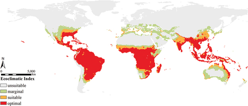
Figure 5. (a) Cold stress map and (b) dry stress map of peanut crops generated from the CLIMEX model. Green cross represents the peanut distribution data taken from GBIF (2017) and ALA (2017).

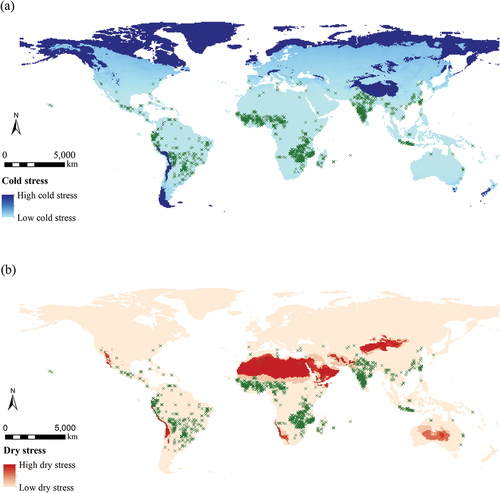
The model also successfully captured peanut distribution data in exotic locations, where the species is cultivated, including China, the United States, India, Indonesia, Myanmar, Thailand, Vietnam, and the Philippines. The peanut distribution in China resulting from CLIMEX model aligns well with the peanut distribution map produced in Yang and Zheng (2016) study, and it captured all major peanut growing areas in China. Some minor growing areas in China, such as Xinjiang, Gansu, Ningxia, Inner Mongolia, and Heilongjiang, were not included in the model due to unfavorable climate conditions for massive peanut planting. These minor growing areas experience cold and arid climates. In India, only small amount of distribution data in the arid region of Rajasthan was not included in the model, due to lack of rainfall and dry stress persistence (Figure 5b). It was found in this study that peanut crop distribution was affected by cold stress, where low temperature limited peanut crop distribution, and dry stress, where low moisture limited peanut crop distribution.

The majority of peanut distribution data in Africa, Central America, and Australia, which was retained for model validation, shows general agreement with the CLIMEX model output (Figure 6). All distribution data in Australia were included in the CLIMEX model and only one outlier data were found in Central America. Closer detail of the African region reveals that 99.3% of peanut records were incorporated in the model. In addition, the majority of the distribution data of these validation areas fell within optimal and suitable areas for peanut planting.

Figure 6. The distribution of peanut crops in validation areas of (a) Central America, (b) Africa, and (c) Australia. Blue dots represent current peanut distribution data.

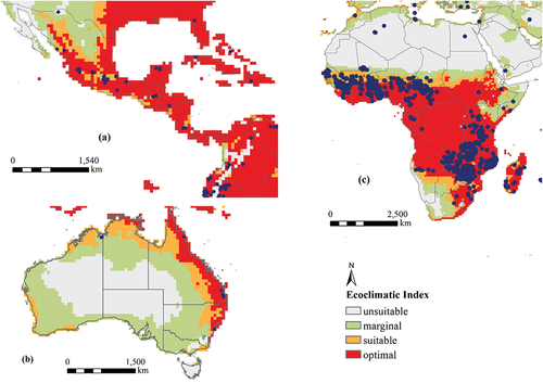
Most of the areas with optimal suitability for growing peanut crops are found in tropical regions, i.e. SouthEast Asia, East India, Central Africa, the northern part of South America, and Central America. However, it has been found that some subtropical and arid regions, including the southern part of China, the eastern part of Australia, the north-eastern part of Argentina, Uruguay, the south-eastern part of the United States, and the eastern parts of South Africa, Zambia, and South Angola, also show optimal suitability. In addition, areas which are categorized as suitable for peanut cultivation are found in subtropical regions, such as the middle-eastern part of the United States and the eastern part of China, and arid regions, such as the northern parts of India and Central Africa (Figure 4). In Australia, current suitable areas for peanut growing are located in the eastern parts of Queensland and New South Wales; the northern parts of Queensland, the Northern Territory, and Western Australia; and the eastern part of Western Australia, which are characterized as tropical and subtropical climate regions (Figure 6).

3.2. Future projections

The results of projections of future peanut cropping areas in Australia using CSIRO-Mk3.0 are shown in Figure 7. A comparison of the projection years shows that there has been a significant increase in unsuitable peanut cropping areas, which is marked by approximately 76% of Australian continent in 2100. In 2030, the projected unsuitable areas only cover the arid region in the middle of Australia, but these unsuitable areas will be expanded throughout the projection years, until in 2100, they are projected to reach the current peanut growing areas in subtropical regions of the eastern part of Queensland and tropical regions of northern Queensland and the Northern Territory. Current peanut planting areas, which will not be suitable in 2100 include Katherine in the Northern Territory and Georgetown, Emerald, St. George, Chinchilla, Inglewood, and Texas in Queensland. These areas are the expansion of peanut growing regions in Australia, due to decreasing productivity in the traditional dryland peanut regions in the South and North Burnett (Chauhan et al. 2013).

Figure 7. The future distribution of peanut crops in Australia using CSIRO-Mk3.0 Global Climate Model, with climate scenarios of the SRES A2.

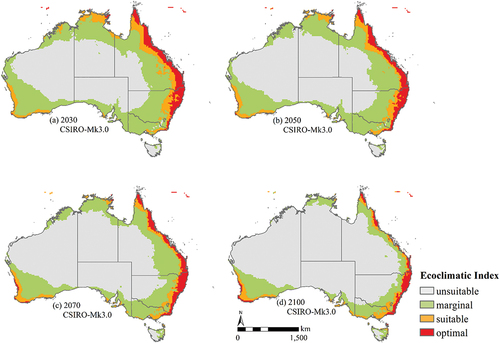
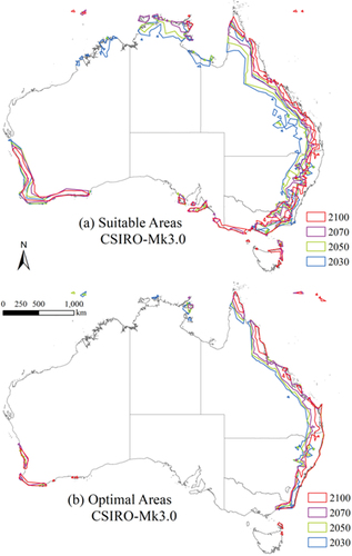
Moreover, the traditional dryland peanut regions, i.e. the South Burnett and the North Burnett, have been projected as marginal peanut growing areas in 2100. In terms of projections for optimal and suitable areas, which are mainly located on the eastern coast of Australia and known as peanut main production regions, there is a significant reduction under the CSIRO-Mk3.0 model (Figure 8). Interestingly, small areas in the south-western part of West Australia and south-eastern parts of New South Wales and Victoria, which are marked as marginal areas in the current peanut distribution, are projected to become suitable areas in 2100 (Figure 8).

Figure 8. The dynamic shifting of projected suitable and optimal areas of peanut crops in Australia using CSIRO-Mk3.0 Global Climate Model in 2030, 2050, 2070, and 2100.

The results of MIROC-H projections in areas of peanut crop suitability in Australia (Figure 9), especially for optimal and suitable areas, are not as dramatic as CSIRO-Mk3.0 projections. Although there is a significant increase in unsuitable peanut areas in 2100, it only accounts for approximately 48% of Australian continent. In addition, unlike CSIRO-Mk3.0 projections, MIROC-H projections of unsuitable areas are mainly concentrated in the middle of Australia, with a smaller effect for tropical regions in the northern part of Australia. The number of current peanut production areas, which will become unsuitable in 2100, according to the MIROC-H projection, is considerably smaller than the number CSIRO-Mk3.0 number. Only two current peanut production areas will be affected: Georgetown in northern Queensland and Katherine in the Northern Territory.

Figure 9. The future distribution of peanut crops in Australia using MIROC-H Global Climate Model, with climate scenarios of the SRES A2.

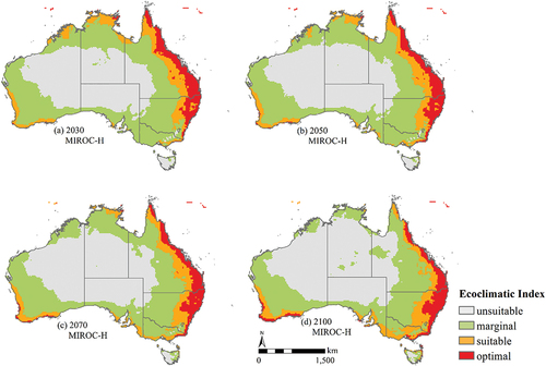
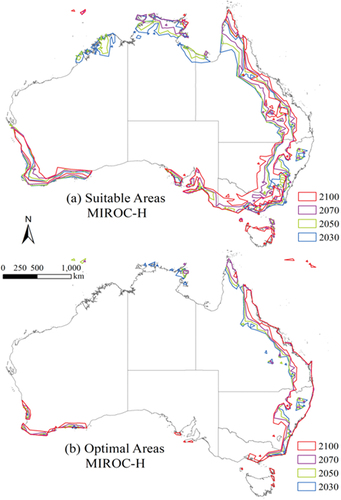
Looking at the dynamic shifting of suitable and optimal areas throughout the projection years (Figure 10), the subtropical regions in the eastern part of Australia where peanuts are mainly produced, i.e. South Burnett, North Burnett, Chinchilla, Inglewood, and Texas, are still categorized as optimal and suitable areas in 2100. Only little change occurs in these regions. Meanwhile, other current peanut production areas, i.e. Emerald and St. George, are projected to be marginal areas in 2100. Moreover, similar to the CSIRO-Mk3.0 projections, some areas in the south-western part of West Australia and south-eastern parts of New South Wales and Victoria will become suitable for peanut cultivation in 2100 according to the MIROC-H projection (Figure 10). However, MIROC-H projection coverage for these regions is larger than the CSIRO-Mk3.0 projection coverage.

Figure 10. The dynamic shifting of projected suitable and optimal areas of peanut crops in Australia using MIROC-H Global climate in 2030, 2050, 2070, and 2100.

In general, the results show a projected reduction in suitable areas for peanut crop planting in Australia under the SRES A2 using two GCMs, CSIRO-Mk3.0 and MIROC-H; although a few areas will experience increasing suitability for peanut planting (Figures 7, 9). Both models, CSIRO-Mk3.0 and MIROC-H, show a decreased trend in optimal, suitable, and marginal areas throughout the projection years (Figure 11). However, CSIRO-Mk3.0 projected a significant reduction from year to year, which could be seen from the decrease of 56% of the marginal areas and almost 50% of the optimal and suitable areas in 2100, compared to 2030. Meanwhile, MIROC-H predicted a small reduction in 2100 compared to 2030 for optimal, suitable, and marginal peanut planting areas, i.e. 5%, 13%, and 15%, respectively. Comparing the two models, the MIROC-H projections for optimal, suitable, and marginal areas are higher than CSIRO-Mk3.0 projections. It should also be noted that, for the MIROC-H projection, marginal areas for peanut cultivation in 2030 are slightly higher than unsuitable areas. Nevertheless, since 2050, unsuitable areas of MIROC-H projection exceed marginal areas, and the trend continues until 2100.

Figure 11. The total areas of future peanut crops using the CSIRO-Mk3.0 (CS) and MIROC-H (MR) projections for 2030, 2050, 2070, and 2100.

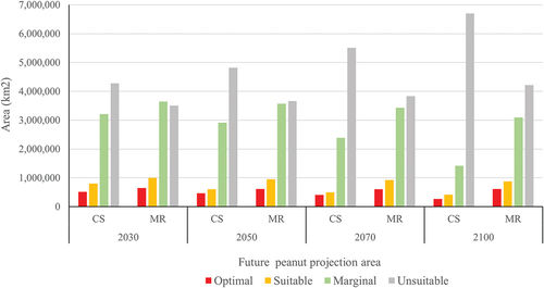
In contrast, there is an increased trend for unsuitable projection areas for both models. However, similar to the trends for other category areas, the increase for MIROC-H in 2100 compared to 2030 is lower than for CSIRO-Mk3.0, which accounted for 20% and 57%, respectively. In general, the CSIRO-Mk3.0 projection for future unsuitable peanut crop areas shows a higher number than the MIROC-H projection, with a trend of an increasing gap between the two models throughout the projection years. The results show that there is a significant difference between projections of unsuitable peanut cropping areas for both models in 2100.

Examining cold stress projections for peanut planting areas, both the CSIRO-Mk3.0 and MIROC-H models forecast almost similar cold stress areas for peanut cultivation. These are located in temperate regions in the south-eastern part of Australia. Specifically, the models predicted a reduction in cold stress areas throughout the projection years. Comparing the two models, the MIROC-H model projected a slightly higher cold stress severity and coverage area than the CSIRO-Mk3.0 model, especially in 2070 and 2100. In terms of dry stress projections, which are mainly located in the arid region of central Australia, the areas affected by dry stress are larger for the CSIRO-Mk3.0 model than the MIROC-H model. Moreover, the CSIRO-Mk3.0 model predicted an increase in dry stress areas throughout the projection years. It is projected that by 2100, dry stress areas will expand to central Queensland, the majority of Western Australia, and tropical regions in the Northern Territory. Meanwhile, the MIROC-H projected a reduction in dry stress in central Australia and a small dry stress increase in the northern part of Western Australia. Analyzing the heat stress, both models projected that Australia will not experience heat stress until 2100. However, comparing the two models, more areas are significantly affected by heat stress in the CSIRO-Mk3.0 projection than the MIROC-H projection, i.e. areas in the northern and middle parts of Australia.

The results of overlaid maps between the two models, CSIRO-Mk3.0 and MIROC-H, show an agreement in the reduction of peanut planting areas in the tropical regions in the northern part of Australia and an increase in the peanut suitability in the temperate regions in the south-eastern part of Australia (Figure 12). While the percentage of unsuitable/marginal agreement areas between two models is moderately constant from 81.09% of Australian continent in 2030 to around 82.87% of Australian continent in 2100, the percentage of optimal/suitable areas decreased from 14.65% of Australian continent in 2030 to 7.51% of Australian continent in 2100. In addition, the overlaid maps also show a disagreement between the two models. For example, in 2100, Chinchilla is categorized as an unsuitable area in the CSIRO-Mk3.0 projection, while the MIROC-H projection included Chinchilla as a suitable area. The disagreement areas increased from 4.26% of Australian continent in 2030 to 9.62% of Australian continent in 2100.

Figure 12. CSIRO-Mk3.0 (CS) and MIROC-H (MR) overlaid map of future distribution of peanut crops in Australia under climate scenarios of the SRES A2.

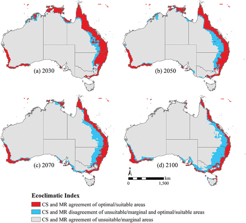
The overlaid maps show that some current peanut cropping areas, i.e. Katherine in the Northern Territory, Georgetown in northern Queensland, St. George in southern Queensland, and Emerald in central Queensland, will be not be suitable for peanut planting in 2100. Meanwhile, two models, i.e. CSIRO-Mk3.0 and MIROC-H, disagreed with the projections in 2100 of other current peanut planting areas in Queensland such as South Burnett, North Burnett, Chinchilla, Inglewood, and Texas.

4. Discussion

4.1. Peanut distribution under current climate

The CLIMEX model produced from this study showed agreement with the majority of the distribution data in both native and exotic ranges, which confirmed the correctness of the selected peanut CLIMEX parameter values. Only small amounts of peanut distribution data, i.e. 2.3%, were not included in the CLIMEX model, which could be peanut herbarium records or errors in GBIF or ALA databases. In addition, the fact that the majority of peanut distribution data were categorized as optimal and suitable peanut planting areas, together with the inclusion of majority peanut distribution data in model validation, has strengthened the validity of the model. Furthermore, it was also found that the peanut distribution produced from this model is consistent with the data of global peanut cropping areas retrieved from the Spatial Production Allocation Model (SPAM 2021).

Although known as moderately drought tolerant crops, peanut crops require at least 600 mm of well-distributed water throughout the growing season for achieving optimal yields. In addition, the crops typically require warm temperatures, i.e. around 25–30°C for vegetative growth and around 22–24°C for generative growth (DPIF 2007). Therefore, as can be seen in the peanut CLIMEX model, tropical regions are the most suitable areas to cultivate peanut crops, although the model also includes some subtropical regions. In fact, the starting point to develop peanut CLIMEX parameters in this study was the CLIMEX wet tropical template parameters, which are provided in the CLIMEX program. In addition, due to the temperature and water requirements as mentioned before, peanut crop distribution was limited by cold and dry stress. As a result, peanut distribution cannot be found in extremely arid regions, such as northern Africa, or in extremely cold regions, such as Northern Europe and Northern America.

Good data sources are important to enhance the reliability of CLIMEX model in projecting the species distribution. It is worth noting that this study included climate ranges of both native and exotic distribution data in a heterogeneous environment to parameterize CLIMEX model of peanut crops. As explained in section 2.4.2, this model parameterization was designed to enhance the model’s ability to project the species’ potential distribution (Kriticos et al. 2015). Some distribution areas could have been missed in the development of the CLIMEX model. However, model development did not only rely on geographical distribution alone but also from field and laboratory data (Kriticos et al. 2015) in the peanut developmental threshold of temperature and moisture levels. This is to ensure that the resulting model’s parameters are biologically responsible.

In addition, climate is not the only factor determining species spatial distribution; other factors such as competition (e.g. natural enemies), habitat (e.g. soil types and host availability), crop price, and land management also play crucial roles (Guoxin, Shibasaki, and Matsumura 2004; Kriticos et al. 2015). Areas with different climates from which species originally grew could be suitable for that species due to the absence of its natural enemies (Kriticos et al. 2015). Thus, to ensure the coverage of all climatic ranges of peanut crops, this study used both native and exotic distributions of peanut crops in developing the CLIMEX model.

The current development of SDMs of invasive species shows a trend of using only the exotic distribution data of the species. One of the criticisms in modeling invasive species using SDMs is that the model could violate the equilibrium assumption (Barbet-Massin et al. 2018). Therefore, the predictive accuracy of SDMs on projecting the invasion of species in exotic places needs to be assessed (Barbet-Massin et al. 2018). To facilitate this assessment, several studies developed their SDMs using two different groups of data, i.e. native and exotic distribution data and exotic distribution data. Barbet-Massin et al. (2018) found that the predictive accuracy of V.v. nigrithorax in its invasive range was slightly better when using exotic data only. Thus, future studies on peanut crops distribution in new expanded agricultural areas might explore the predictive accuracy of SDMs by employing specifically exotic distribution data.

Differentiating input data into two groups can provide an opportunity to explore environmental drivers of species distribution in specific areas. O’Mahony, de la Torre Cerro, and Holloway (2021) discovered that modeling the distribution of Asparagopsis species using the exotic distribution data alone produced broader projection areas than modeling it using both native and exotic distribution data. Their findings suggest the possibility of niche shift in the species’ suitability areas, which are driven by the important environmental variables. Therefore, future research in the projection of peanut crops distribution might explore the possibility of running the model separately for each group of data to identify the most important environmental drivers in each group. In addition, as peanut crops are cultivated all around the world, running the model specifically for each distribution group can provide an opportunity to identify additional climatic niches of peanut crops (if any).

4.2. Peanut distribution under future climate scenarios

The results of this study and other crop distribution studies, such as wheat and cotton (Shabani and Kotey 2015), common bean (Ramirez-Cabral, Kumar, and Taylor 2016), tomato (Silva et al. 2017), oil palm (Paterson et al. 2015), and date palm (Shabani, Kumar, and Taylor 2015), confirm the effects of climate change on crop distribution. Climate is one of the significant factors in determining crop planting suitability (Anwar et al. 2013). Currently, regions with low-temperature constraints, such as high mid-latitude countries, may increase their agricultural productivity, while current productive areas in mid-latitude continental countries may experience productivity decrease due to moisture stress increase. In addition, countries in lower middle and low latitudes, which have limited production capacity, will experience further crop stress as a result of climate change (Parry, Porter, and Carter 1990).

CLIMEX model projections on future peanut cropping areas in Australia showed a decrease in suitable peanut planting areas and the emergence of new suitable peanut planting areas for two climate models used in this study, i.e. CSIRO-Mk3.0 and MIROC-H. In the future, it is predicted that dry stress will limit peanut distribution in Australia, since the results of this study have shown that the increase in unsuitable areas is in line with the increase in projected dry stress. This study also found that dry stress projection coverage for CSIRO-Mk3.0 was larger than MIROC-H coverage, which explains the larger coverage of unsuitable areas for CSIRO-Mk3.0 than MIROC-H coverage. In addition, the influence of heat stress occurrence in 2100 also contribute for the decrease in suitable areas for peanut planting in Australia. Interestingly, some areas in the south-western part of Western Australia and south-eastern parts of New South Wales and Victoria, which are currently not suitable for peanut planting due to cold stress occurrence, are predicted to be suitable in the future. It is predicted that cold stress limitation in these areas will be reduced in the future, since the areas will become warmer due to climate change.

The results of this study were consistent with the results of a future distribution study of another legume crop, the common bean (Phaseolus vulgaris L.), which also originated in South America. In their study, Ramirez-Cabral, Kumar, and Taylor (2016) used two climate models, CSIRO-Mk3.0 and MIROC-H, in projecting the future common bean distribution. Their findings produced similar results to our study, i.e. there is a slight increase in suitable common bean planting area in the New South Wales coast and the southern coast of Western Australia, and CSIRO-Mk3.0 (rather than MIROC-H) projected a less suitable area for common bean cultivation in Australia in 2100. The differences in the model output from these two climate models are understandable, given that they were developed by two different institutions. CSIRO-M3.0 was developed by CSIRO, Australia, while MIROC-H was developed by the Center for Climate Research, Japan. In a study to measure the performance of AR4 GCMs in Australia, it was found that CSIRO-Mk3.0 was among the best models in simulating the probability of temperature minimum (T_min), while MIROC-H was among the best models in simulating the probability of temperature maximum (T_max) (Perkins et al. 2007). These results increase the confidence that the models can simulate future climate over Australia with a greater proportion, and thus confirm the model’s skill.

Analogous to other CLIMEX studies used to project future cotton and wheat distribution in Australia (Shabani and Kotey 2015), the projections of peanut planting areas produced from CSIRO-Mk3.0 and MIROC-H were overlaid to identify common areas between the two models. This method will enhance the likelihood of projections in the future, and thus possible errors can be minimized. Traditionally, in Australia, peanut crops are planted in the South Burnett and North Burnett regions under dryland conditions. However, due to recurring droughts in those regions, peanut areas have been expanded into Katherine in the Northern Territory and areas in the central and northern parts of Queensland, such as Georgetown, the Atherton Tablelands, Emerald, Chinchilla, St. George, Childers, Inglewood, Texas, and Bundaberg (Chauhan et al. 2013). Unfortunately, based on the overlaid projections of future suitable peanut planting areas using CLIMEX model, some of these expansion regions will experience unsuitable climatic conditions for peanut growth.

The overlaid CLIMEX model maps from CSIRO-Mk3.0 and MIROC-H climate models indicate that Katherine in the Northern Territory and Georgetown, Emerald, and St. George in Queensland will have low suitability or will not be suitable for peanut planting areas. Only Bundaberg, Mackay, the Atherton Tableland, and Childers in Queensland can be reserved as suitable or optimal areas in 2100. Meanwhile, both CSIRO-Mk3.0 and MIROC-H models disagreed on climate suitability in 2100 for other peanut regions, including the traditional peanut planting areas of South Burnett and North Burnett, where one model included a region as an optimal/suitable area, while the other model included it as an unsuitable/marginal area. Indeed, this fact gives a warning of the potential negative impacts of climate change in the current peanut growing regions in Australia. Currently, more than 90% of peanut growing regions in Australia, which supply the majority of the peanut domestic market, are located in Queensland (Wright, Wieck, and O’Connor 2017). Therefore, it is important to develop strategic measures to overcome and manage the economic impacts of the projected shifting climate suitability of the majority of current peanut growing regions.

Based on the projections, future peanut distribution in Australia will be limited by the occurrence of dry stress, which could have unfavorable effects for peanut crops. Although known as moderately drought tolerant, peanut crops require readily available moisture throughout their development stages, especially in the flowering and pod formation stages (DPIF 2007). Inadequate water supply during flowering will reduce pod yield, while severe drought stress during the pod filling stage will lead to more severe yield reduction (Wright, Hubick, and Farquhar 1991). Recurrence of water deficit during the late season decreases yield, reduces peanut quality, and increases the possibility of aflatoxin disease contamination (Kambiranda et al. 2011). Peanut seed physiological activity is reduced with the occurrence of drought stress, thus it becomes more susceptible to fungal invasion, such as aspergillus invasion that leads to aflatoxin disease (Kambiranda et al. 2011).

As a result of frequent water deficit, crops experience anatomical changes, i.e. reduction in size of cell and intercellular spaces, cell walls thickening, and larger development of epidermal tissue. In addition, severe water deficits could also influence a crop’s metabolic process, i.e. reduction in enzymatic activity (Kambiranda et al. 2011). Shahenshah and Isoda (2010) found that drought stress in peanut caused an increase in leaf temperature and non-photochemical quenching. Moreover, it leads to a reduction in water content per unit leaf area, chlorophyll content, and maximum quantum yield of the photosystem. Furthermore, peanut crops also experience an increase in root dry weight with a small reduction in leaf area when they suffer drought stress (Shahenshah and Isoda 2010).

Therefore, it is important to take strategic measures to anticipate the future shifting suitable areas of peanut crops in Australia, especially since the majority of current peanut planting areas will be negatively affected. One measure that has been taken and is still in progress is the development of drought tolerant varieties. Currently, drought tolerant peanut genotypes are screened using advanced molecular tools, which involve studies on the peanut at the molecular and cellular levels (Kambiranda et al. 2011). Although an improved peanut genotype that can tolerate drought stress has been developed, the process still needs to continue to develop advanced genotypes (Kambiranda et al. 2011). Another measure that can be considered is to apply and improve irrigation and greenhouse technologies, although economic constraints must also be considered.

It should be noted that careful considerations should be taken in interpreting the results of this study, since the CLIMEX model only considers climatic factors in determining the current and future distributions of the species. Soberón and Townsend Peterson (2005) mentioned three factors that affect the geographical distribution of a species: first, environmental factors, which majority consist of abiotic factors such as climate, topography, and solar radiation; second, biotic factors such as competitors, predators, and mutualists; and third, accessible areas. Non-climatic factors that could limit species distribution, such as biotic interactions (e.g. competition and predator), habitats (e.g. presence of suitable hosts, soil types, and humans), and topographic elements (Kriticos et al. 2015), were likewise not considered in CLIMEX modeling. In addition, the model development of this study did not consider the application of irrigation and the use of greenhouse technologies in peanut crops, which could increase the suitable areas of peanut crop planting. It should also be noted that there could be some limitations of CLIMEX model, such as in capturing areas near the boundary or threshold of climate parameters used in the model.

5. Conclusion

In this study, we have successfully developed CLIMEX model parameters for peanut crops, which are found to be consistent with the current peanut geographic distribution. In addition, using CSIRO-Mk3.0 and MIROC-H Global Climate Models under the climate scenarios of the SRES A2, CLIMEX model projections for future peanut distribution in Australia show an increase in unsuitable areas for peanut cultivation. Specifically, the projection of unsuitable peanut cultivation areas in 2100 is higher for CSIRO-Mk3.0 (i.e. 76% of the Australian continent) than MIROC-H (48%). In the future, dry stress is projected to increase and will cause limitations of suitable peanut areas. The overlaid maps of CSIRO-Mk3.0 and MIROC-H models have projected that in 2100, some existing peanut cultivation areas, namely, Katherine (the Northern Territory) and Georgetown, Emerald, and St. George (Queensland), will become unsuitable for peanut cultivation. Only peanut cropping areas in Bundaberg, Mackay, the Atherton Tableland, and Childers in Queensland are projected to be suitable or optimal for peanut cultivation in 2100. Meanwhile, CSIRO-Mk3.0 and MIROC-H models disagreed on climatic suitability in 2100 for other peanut cropping areas, such as the traditional peanut planting areas in South and North Burnett, Chinchilla, Inglewood, and Texas. The future peanut distribution maps resulting from this study will provide valuable contributions in long-term planning of peanut cultivation in Australia, especially with regard to the projected unsuitable areas for the majority of current peanut cultivation regions. However, further work is needed to include non-climatic factors, such as topography, soil type, and biotic interactions, to further increase the accuracy and robustness of the projected spatial distribution of peanut cropping areas.

Acknowledgements

We would like to thank the Australian Government for the Australia Awards Scholarship awarded to the first author. We would also like to acknowledge GBIF and ALA as data sources for this study, and the helpful proofreading work of Dr. Barbara Harmes.

Disclosure statement

No potential conflict of interest was reported by the authors.

Data availability statement

The peanut distribution data can be obtained from the Global Biodiversity Information Facility (GBIF, http://www.gbif.org/species) and the Atlas of Living Australia (ALA, http://www.ala.org.au/). The climate variable data used to run the CLIMEX model was retrieved from the CliMond database (https://www.climond.org/ClimateData.aspx).

Additional information

Funding

This research did not receive any specific grant from funding agencies in the public, commercial, or not-for-profit sectors.

Notes on contributors

Haerani Haerani

Haerani Haerani is a Senior Lecturer at the Department of Agricultural Engineering, Universitas Hasanuddin, Indonesia. She received her PhD from the University of Southern Queensland, Australia. Her research interests include remote sensing and geospatial analyses in agriculture.

Armando Apan

Armando Apan is a Professor at the School of Surveying and Built Environment, University of Southern Queensland, Australia, and an Adjunct Professor at the Institute of Environmental Science and Meteorology, University of the Philippines Diliman, the Philippines. He received his PhD from Monash University, Australia. His research interests focus on the use of remote sensing and GIS in ecology, forestry, agriculture, and environmental management.

Thong Nguyen-Huy

Thong Nguyen-Huy is a Post-doctoral fellow at the SQNNSW Drought Resilience Adoption and Innovation Hub, University of Southern Queensland, Australia. He received his PhD from the University of Southern Queensland, Australia. His research interests include modeling and data analysis and developing and applying novel statistical models, AI algorithms, and remote sensing techniques.

Badri Basnet

Badri Basnet is a Senior Lecturer at the School of Surveying and Built Environment, University of Southern Queensland, Australia. He received his PhD from the University of Southern Queensland, Australia. His research interests focus on the development and use of open educational resources in GIS education and free and open-source software for geo-spatial.

References

- ABARES. 2016. “Australian Crop Report.” Canberra: Australian Bureau of Agricultural and Resource Economics and Sciences.
- ABARES. 2019. “National Scale Land Use of Australia 2010-11.” ABARES, Accessed 13 March 2019. http://www.agriculture.gov.au/abares/aclump.
- ALA. 2017. “Atlas of Living Australia.” Accessed 17 August 2017. http://www.ala.org.au/.
- Al-Hanbali, A., K. Shibuta, B. Alsaaideh, and Y. Tawara. 2021. “Analysis of the Land Suitability for Paddy Fields in Tanzania Using a GIS-Based Analytical Hierarchy Process.” Geo-Spatial Information Science 25: 1–17. doi:10.1080/10095020.2021.2004079.
- Anwar, M. R., D. L. Liu, I. Macadam, and G. Kelly. 2013. “Adapting Agriculture to Climate Change: A Review.” Theoretical and Applied Climatology 113 (1–2): 225–245. doi:10.1007/s00704-012-0780-1.
- Austin, M. P. 2002. “Spatial Prediction of Species Distribution: An Interface Between Ecological Theory and Statistical Modelling.” Ecological modelling 157 (2–3): 101–118. doi:10.1016/S0304-3800(02)00205-3.
- Barbet-Massin, M., Q. Rome, C. Villemant, and F. Courchamp. 2018. “Can Species Distribution Models Really Predict the Expansion of Invasive Species?” PLoS One 13 (3): e0193085.
- Beaumont, L. J., L. Hughes, and A. J. Pitman. 2008. “Why is the Choice of Future Climate Scenarios for Species Distribution Modelling Important?” Ecology letters 11: 1135–1146.
- Bell, M. J., R. Shorter, and R. Mayer. 1991. “Cultivar and Environmental Effects on Growth and Development of Peanuts (Arachis Hypogaea L.). I. Emergence and Flowering.” Field Crops Research 27 (1–2): 17–33. doi:10.1016/0378-4290(91)90019-R.
- Bernstein, L., P. Bosch, O. Canziani, Z. Chen, R. Christ, O. Davidson, W. Hare, S. Huq, D. Karoly, and V. Kattsov. 2008. Climate Change 2007: Synthesis Report: An Assessment of the Intergovernmental Panel on Climate Change. Valencia: IPCC.
- Canadell, J. G., C. P. Meyer, G. D. Cook, A. Dowdy, P. R. Briggs, J. Knauer, A. Pepler, and V. Haverd. 2021. “Multi-Decadal Increase of Forest Burned Area in Australia is Linked to Climate Change.” Nature communications 12 (1): 1–11. doi:10.1038/s41467-021-27225-4.
- Chakraborty, S., A. V. Tiedemann, and P. S. Teng. 2000. “Climate Change: Potential Impact on Plant Diseases.” Environmental Pollution 108 (3): 317–326. doi:10.1016/S0269-7491(99)00210-9.
- Chauhan, Y. S., G. C. Wright, D. Holzworth, R. C. Rachaputi, and J. O. Payero. 2013. “AQUAMAN: A Web-Based Decision Support System for Irrigation Scheduling in Peanuts.” Irrigation Science 31 (3): 271–283. doi:10.1007/s00271-011-0296-y.
- Coakley, S. M., H. Scherm, and S. Chakraborty. 1999. “Climate Change and Plant Disease Management.” Annual Review of Phytopathology 37 (1): 399–426. doi:10.1146/annurev.phyto.37.1.399.
- Craufurd, P. Q., P. V. Vara Prasad, V. G. Kakani, T. R. Wheeler, and S. N. Nigam. 2003. “Heat Tolerance in Groundnut.” Field Crops Research 80 (1): 63–77. doi:10.1016/S0378-4290(02)00155-7.
- Crosthwaite, I. 1994. Peanut Growing in Australia. Brisbane: Department of Primary Industries.
- CSIRO, and BoM. 2015. “Climate Change in Australia Information for Australia’s Natural Resource Management Regions: Technical Report.” Australia: CSIRO and BoM.
- CSIRO, and BoM. 2020. “State of the Climate 2020.” Australia: CSIRO and BoM.
- DERM. 2010. “Climate Change in Queensland - What the Science is Telling Us.” Brisbane: DERM - State of Queensland.
- DPIF. 2007. “Best Management Practices for Peanuts.” Brisbane: Department of Primary Industries and Fisheries - The State of Queensland.
- Elith, J., and J. R. Leathwick. 2009. “Species Distribution Models: Ecological Explanation and Prediction Across Space and Time.” Annual Review of Ecology, Evolution, and Systematics 40 (1): 677–697. doi:10.1146/annurev.ecolsys.110308.120159.
- Fawzy, S., A. I. Osman, J. Doran, and D. W. Rooney. 2020. “Strategies for Mitigation of Climate Change: A Review.” Environmental Chemistry Letters 18: 2069–2094. doi:10.1007/s10311-020-01059-w.
- GBIF. 2017. “Global Biodiversity Information Facility.” Accessed 5 August 2017. http://www.gbif.org/species.
- Geoscience Australia. 2018. “Area of Australia - State and Territories.” Geoscience Australia, Accessed 3 April 2018. http://www.ga.gov.au/scientific-topics/national-location-information/dimensions/area-of-australia-states-and-territories.
- Gogol-Prokurat, M. 2011. “Predicting Habitat Suitability for Rare Plants at Local Spatial Scales Using a Species Distribution Model.” Ecological Applications 21 (1): 33–47. doi:10.1890/09-1190.1.
- Gornall, J., R. Betts, E. Burke, R. Clark, J. Camp, K. Willett, and A. Wiltshire. 2010. “Implications of Climate Change for Agricultural Productivity in the Early Twenty-First Century.” Philosophical Transactions of the Royal Society B: Biological Sciences 365 (1554): 2973–2989. doi:10.1098/rstb.2010.0158.
- GRDC. 2014. “GRDC Grownotes: Peanuts.” GRDC - Grains Research and Development Corporation.
- Guoxin, T., R. Shibasaki, and K. Matsumura. 2004. “Development of a GIS-Based Decision Support System for Assessing Land Use Status.” Geo-Spatial Information Science 7 (1): 72–78. doi:10.1007/BF02826679.
- Halder, D., S. Kheroar, R. Kumar Srivastava, and R. Kumar Panda. 2020. “Assessment of Future Climate Variability and Potential Adaptation Strategies on Yield of Peanut and Kharif Rice in Eastern India.” Theoretical and Applied Climatology 140 (3): 823–838. doi:10.1007/s00704-020-03123-5.
- Heikkinen, R. K., M. Luoto, M. B. Araújo, R. Virkkala, W. Thuiller, and M. T. Sykes. 2006. “Methods and Uncertainties in Bioclimatic Envelope Modelling Under Climate Change.” Progress in Physical Geography 30 (6): 751–777. doi:10.1177/0309133306071957.
- Hijmans, R. J., S. E. Cameron, J. L. Parra, P. G. Jones, and A. Jarvis. 2005. “Very High Resolution Interpolated Climate Surfaces for Global Land Areas.” International Journal of Climatology 25 (15): 1965–1978. doi:10.1002/joc.1276.
- IPCC. 2014. Climate Change 2014: Synthesis Report - Contribution of Working Groups I, II and III to the Fifth Assessment Report of the Intergovernmental Panel on Climate Change. edited by Rajendra K. Pachauri and Leo Meyer. Geneva: IPCC.
- IPCC. 2018. ”Global Warming of 1.5°C: An IPCC Special Report on the Impacts of Global Warming of 1.5°C Above Pre-Industrial Levels and Related Global Greenhouse Gas Emission Pathways, in the Context of Strengthening the Global Response to the Threat of Climate Change, Sustainable Development, and Efforts to Eradicate Poverty.” In Summary for Policymakers, edited by T. Waterfield, P. Zhai, V. Masson-Delmonte, H.-O. Portner, D. Roberts, J. Skea, P. Shukla, A. Pirani, W. Moufouma-Okia, C. Pean, R. Pidcock, S. Connors, J. Matthews, Y. Chen, X. Zhou, M. Gomis, E. Lonnoy, T. Maycock, and M. Tignor, 3–24. Cambridge and New York: In Press.
- IPCC. 2021. “Climate Change 2021: The Physical Science Basis Contribution of Working Group I to the Sixth Assessment Report of the Intergovernmental Panel on Climate Change.” In Summary for Policymakers, edited by V. Masson-Delmotte, P. Zhai, A. Pirani, S. L. Connors, C. Pean, Y. Chen, L. Goldfarb, 4–31. In Press.
- Joshi, P., N. Sheena, R. Asha, and J. Aniruddha. 2011. “Landscape Characterization of Sariska National Park (India) and Its Surroundings.” Geo-Spatial Information Science Ghosh 14 (4): 303–310. doi:10.1007/s11806-011-0557-1.
- Kambiranda, D. M., H. K. Vasanthaiah, R. Katam, A. Ananga, S. M. Basha, and K. Naik. 2011. “Impact of Drought Stress on Peanut (Arachis Hypogaea L.) Productivity and Food Safety.” In Plants and environment, edited by H. Vasanthaiah, 249–272. Rijeka, Croatia: InTech.
- Ketring, D. L. 1984. “Temperature Effects on Vegetative and Reproductive Development of Peanut.” Crop Science 24 (5): 877–882. doi:10.2135/cropsci1984.0011183X002400050012x.
- King, A. D., D. J. Karoly, and B. J. Henley. 2017. “Australian Climate Extremes at 1.5 C and 2 C of Global Warming.” Nature Climate Change 7 (6): 412–416. doi:10.1038/nclimate3296.
- King, A. D., N. P. Klingaman, L. V. Alexander, M. G. Donat, N. C. Jourdain, and P. Maher. 2014. “Extreme Rainfall Variability in Australia: Patterns, Drivers, and Predictability.” Journal of Climate 27 (15): 6035–6050. doi:10.1175/JCLI-D-13-00715.1.
- Kriticos, D. J., and A. Leriche. 2010. “The Effects of Climate Data Precision on Fitting and Projecting Species Niche Models.” Ecography 33 (1): 115–127. doi:10.1111/j.1600-0587.2009.06042.x.
- Kriticos, D. J., G. F. Maywald, T. Yonow, E. J. Zurcher, N. I. Herrmann, and R. W. Sutherst. 2015. “Climex Version 4: Exploring the Effects of Climate on Plants, Animals and Diseases.” Canberra: CSIRO.
- Kriticos, D. J., and R. P. Randall. 2001. “A Comparison of Systems to Analyse Potential Weed Distributions.” In Weed risk assessment, edited by R. H. Groves, F. D. Panetta, and J. G. Virtue, 61–79. Melbourne: CSIRO Publishing.
- Kriticos, D. J., B. L. Webber, A. Leriche, N. Ota, I. Macadam, J. Bathols, and J. K. Scott. 2012. “CliMond: Global High-resolution Historical and Future Scenario Climate Surfaces for Bioclimatic Modelling.” Methods in Ecology and Evolution 3 (1): 53–64. doi:10.1111/j.2041-210X.2011.00134.x.
- Leong, S. K., and C. K. Ong. 1983. “The Influence of Temperature and Soil Water Deficit on the Development and Morphology of Groundnut (Arachis Hypogaea L.).” Journal of Experimental Botany 34 (11): 1551–1561. doi:10.1093/jxb/34.11.1551.
- Lindsay Corporation. 2010. “Increasing Peanut Yields Through Efficient Irrigation Solutions - Higher Yields, Lower Costs, Precision Application.” Omaha, Nebraska, The USA: Lindsay Corporation.
- Liu, Z., P. Yang, H. Tang, W. Wenbin, L. Zhang, Y. Qiangyi, and L. Zhengguo. 2015. “Shifts in the Extent and Location of Rice Cropping Areas Match the Climate Change Pattern in China During 1980–2010.” Regional Environmental Change 15 (5): 919–929. doi:10.1007/s10113-014-0677-x.
- Manning, M. R., J. Edmonds, S. Emori, K. H. Arnulf Grubler, F. Joos, M. Kainuma, et al. 2010. “Misrepresentation of the IPCC CO2 Emission Scenarios.” Nature geoscience 3 (6): 376–377. doi:10.1038/ngeo880.
- Meinke, H., R. C. Stone, and G. L. Hammer. 1996. “SOI Phases and Climatic Risk to Peanut Production: A Case Study for Northern Australia.” International Journal of Climatology 16 (7): 783–789. doi:10.1002/(SICI)1097-0088(199607)16:7<783:AID-JOC58>3.0.CO;2-D.
- Nakicenovic, N., O. Davidson, G. Davis, A. Grubler, T. Kram, E. Lebre La Rovere, B. Metz, et al. 2000. IPCC Special Report on Emissions Scenarios (SRES), a Special Report of Working Group III of the Intergovernmental Panel on Climate Change: Intergovernmental Panel on Climate Change.
- Nguyen-Huy, T., R. C. Deo, S. Mushtaq, J. Kath, and S. Khan. 2018. “Copula-Based Agricultural Conditional Value-At-Risk Modelling for Geographical Diversifications in Wheat Farming Portfolio Management.” Weather and Climate Extremes 21: 76–89. doi:10.1016/j.wace.2018.07.002.
- Nguyen-Huy, T., J. Kath, S. Mushtaq, D. Cobon, G. Stone, and R. Stone. 2020. “Integrating El Niño-Southern Oscillation Information and Spatial Diversification to Minimize Risk and Maximize Profit for Australian Grazing Enterprises.” Agronomy for Sustainable Development 40 (1): 1–11. doi:10.1007/s13593-020-0605-z.
- Nicholls, N., W. Drosdowsky, and B. Lavery. 1997. “Australian Rainfall Variability and Change.” Weather 52 (3): 66–72. doi:10.1002/j.1477-8696.1997.tb06274.x.
- O’Mahony, J., R. de la Torre Cerro, and P. Holloway. 2021. “Modelling the Distribution of the Red Macroalgae Asparagopsis to Support Sustainable Aquaculture Development.” AgriEngineering 3 (2): 251–265. doi:10.3390/agriengineering3020017.
- Parry, M. L., J. H. Porter, and T. R. Carter. 1990. “Agriculture: Climatic Change and Its Implications.” Trends in Ecology & Evolution 5 (9): 318–322. doi:10.1016/0169-5347(90)90090-Z.
- Paterson, R. R., M. Lalit Kumar, S. Taylor, and N. Lima. 2015. “Future Climate Effects on Suitability for Growth of Oil Palms in Malaysia and Indonesia.” Scientific reports 5: 14457. doi:10.1038/srep14457.
- Perkins, S. E., A. J. Pitman, N. J. Holbrook, and J. McAneney. 2007. “Evaluation of the AR4 Climate Models’ Simulated Daily Maximum Temperature, Minimum Temperature, and Precipitation Over Australia Using Probability Density Functions.” Journal of Climate 20 (17): 4356–4376. doi:10.1175/JCLI4253.1.
- Potgieter, A., H. Meinke, A. Doherty, V. O. Sadras, G. Hammer, S. Crimp, and D. Rodriguez. 2013. “Spatial Impact of Projected Changes in Rainfall and Temperature on Wheat Yields in Australia.” Climatic Change 117 (1–2): 163–179. doi:10.1007/s10584-012-0543-0.
- Rahman, M., and S. Saha. 2009. “Spatial Dynamics of Cropland and Cropping Pattern Change Analysis Using Landsat TM and IRS P6 LISS III Satellite Images with GIS.” Geo-Spatial Information Science 12 (2): 123–134. doi:10.1007/s11806-009-0249-2.
- Ramirez-Cabral, N. Y. Z., L. Kumar, and S. Taylor. 2016. “Crop Niche Modeling Projects Major Shifts in Common Bean Growing Areas.” Agricultural and Forest Meteorology 218: 102–113. doi:10.1016/j.agrformet.2015.12.002.
- Sarkar, A., A. Ghosh, and P. Banik. 2014. “Multi-Criteria Land Evaluation for Suitability Analysis of Wheat: A Case Study of a Watershed in Eastern Plateau Region, India.” Geo-Spatial Information Science 17 (2): 119–128. doi:10.1080/10095020.2013.774106.
- Scheffers, B. R., L. De Meester, T. C. Bridge, A. A. Hoffmann, J. M. Pandolfi, R. T. Corlett, S. H. Butchart, P. Pearce-Kelly, K. M. Kovacs, and D. Dudgeon. 2016. “The Broad Footprint of Climate Change from Genes to Biomes to People.” Science 354 (6313). doi:10.1126/science.aaf7671.
- Shabani, F., and B. Kotey. 2015. “Future Distribution of Cotton and Wheat in Australia Under Potential Climate Change.” The Journal of Agricultural Science 154 (2): 175–185. doi:10.1017/S0021859615000398.
- Shabani, F., L. Kumar, and S. Taylor. 2014. “Projecting Date Palm Distribution in Iran Under Climate Change Using Topography, Physicochemical Soil Properties, Soil Taxonomy, Land Use, and Climate Data.” Theoretical and Applied Climatology 118 (3): 553–567. doi:10.1007/s00704-013-1064-0.
- Shabani, F., L. Kumar, and S. Taylor. 2015. “Distribution of Date Palms in the Middle East Based on Future Climate Scenarios.” Experimental Agriculture 51 (2): 244–263. doi:10.1017/S001447971400026X.
- Shahenshah, and A. Isoda. 2010. “Effects of Water Stress on Leaf Temperature and Chlorophyll Fluorescence Parameters in Cotton and Peanut.” Plant production science 13 (3): 269–278. doi:10.1626/pps.13.269.
- Silva, R. S., L. Kumar, F. Shabani, and M. C. Picanço. 2017. “Assessing the Impact of Global Warming on Worldwide Open Field Tomato Cultivation Through CSIRO-Mk3.0 Global Climate Model.” The Journal of Agricultural Science 155 (3): 407–420. doi:10.1017/S0021859616000654.
- Soberón, J., and A. Townsend Peterson. 2005. “Interpretation of Models of Fundamental Ecological Niches and Species’ Distributional Areas.” Biodiversity Informatics 2: 1–10. doi:10.17161/bi.v2i0.4.
- SPAM. 2021. “Spatial Production Allocation Model.” Accessed 10 June 2021. https://www.mapspam.info/.
- Steffen, W., L. Hughes, V. Sahajwalla, and G. Hueston. 2012. “The Critical Decade: Queensland Climate Impacts and Opportunities.” Canberra: Climate Comission Secretariat (Department of Climate Change and Energy Efficiency).
- Suppiah, R., K. J. Hennessy, P. H. Whetton, K. McInnes, I. Macadam, J. Bathols, J. Ricketts, and C. M. Page. 2007. “Australian Climate Change Projections Derived from Simulations Performed for the IPCC 4th Assessment Report.” Australian Meteorological Magazine 56 (3): 131–152.
- Sutherst, R. W. 2003. “Prediction of Species Geographical Ranges.” Journal of Biogeography 30 (6): 805–816. doi:10.1046/j.1365-2699.2003.00861.x.
- Sutherst, R. W., and G. F. Maywald. 1985. “A Computerised System for Matching Climates in Ecology.” Agriculture, Ecosystems & Environment 13 (3–4): 281–299. doi:10.1016/0167-8809(85)90016-7.
- Tang, C., B. Morel, M. Wild, B. Pohl, B. Abiodun, and M. Bessafi. 2019. “Numerical Simulation of Surface Solar Radiation Over Southern Africa. Part 1: Evaluation of Regional and Global Climate Models.” Climate Dynamics 52 (1): 457–477. doi:10.1007/s00382-018-4143-1.
- Taylor, S., L. Kumar, N. Reid, and D. J. Kriticos. 2012. “Climate Change and the Potential Distribution of an Invasive Shrub, Lantana Camara L.” PLoS One 7 (4): e35565. doi:10.1371/journal.pone.0035565.
- Ujoh, F., T. Igbawua, and M. Ogidi Paul. 2019. “Suitability Mapping for Rice Cultivation in Benue State, Nigeria Using Satellite Data.” Geo-Spatial Information Science 22 (4): 332–344. doi:10.1080/10095020.2019.1637075.
- UNFCCC. 2021. “Glasgow Climate Pact.” In Glasgow: COP26.
- Vara Prasad, P. V., K. J. Boote, L. Hartwell Allen, and J. M. Thomas. 2003. “Super-optimal Temperatures are Detrimental to Peanut (Arachis Hypogaea L.) Reproductive Processes and Yield at Both Ambient and Elevated Carbon Dioxide.” Global Change Biology 9 (12): 1775–1787. doi:10.1046/j.1365-2486.2003.00708.x.
- Vara Prasad, P. V., P. Q. Craufurd, and R. J. Summerfield. 2000. “Effect of High Air and Soil Temperature on Dry Matter Production, Pod Yield and Yield Components of Groundnut.” Plant and Soil 222 (1–2): 231–239. doi:10.1023/A:1004793220787.
- Williams, J. H., and K. J. Boote. 1995. “Physiology and Modeling - Predicting the Unpredictable Legume.” In Advances in Peanut Science, edited by H. E. Patee and H. T. Stalker, 301–353. Stillwater, Oklahoma: American Peanut Research and Education Society.
- WMO. 2010. “Guide to Agricultural Meteorological Practices (GAMP) WMO - No. 134.” Geneva: World Meteorological Organization.
- Wright, G. C., K. T. Hubick, and G. D. Farquhar. 1991. “Physiological Analysis of Peanut Cultivar Response to Timing and Duration of Drought Stress.” Australian Journal of Agricultural Research 42 (3): 453–470. doi:10.1071/AR9910453.
- Wright, D. L., B. Tillman, E. Jowers, J. Marois, J. A. Ferrell, T. Katsvairo, and E. B. Whitty. 2009. “Management and Cultural Practices for Peanuts.” In SS-AGR-74 UF/IFAS Extension University of Florida. Gainesville, Florida.
- Wright, G., L. Wieck, and D. O’Connor. 2017. “Peanut Production Guide.” Peanut Company of Australia.
- Yang, T., and Y. Zheng. 2016. “State and Trends of Oil Crops Production in China.” Oilseeds and Fats, Crops and Lipids 23 (6): D603. doi:10.1051/ocl/2016046.
- Zhao, C., B. Liu, S. Piao, X. Wang, D. B. Lobell, Y. Huang, M. Huang, Y. Yao, S. Bassu, and P. Ciais. 2017. “Temperature Increase Reduces Global Yields of Major Crops in Four Independent Estimates.” Proceedings of the National Academy of Sciences 114 (35): 9326–9331. doi:10.1073/pnas.1701762114.