Lockdown lifted: measuring spatial resilience from London’s public transport demand recovery

ABSTRACT

The disruptive effects of the COVID-19 pandemic has rapidly shifted how individuals navigate in cities. Governments are concerned that travel behavior will shift toward a car-driven and homeworking future, shifting demand away from public transport use. These concerns place the recovery of public transport in a possible crisis. A resilience perspective may aid the discussion around recovery – particularly one that deviates from pre-pandemic behavior. This paper presents an empirical study of London’s public transport demand and introduces a perspective of spatial resilience to the existing body of research on post-pandemic public transport demand. This study defines spatial resilience as the rate of recovery in public transport demand within census boundaries over a period after lockdown restrictions were lifted. The relationship between spatial resilience and urban socioeconomic factors was investigated by a global spatial regression model and a localized perspective through Geographically Weighted Regression (GWR) model. In this case study of London, the analysis focuses on the period after the first COVID-19 lockdown restrictions were lifted (June 2020) and before the new restrictions in mid-September 2020. The analysis shows that outer London generally recovered faster than inner London. Factors of income, car ownership and density of public transport infrastructure were found to have the greatest influence on spatial patterns in resilience. Furthermore, influential relationships vary locally, inviting future research to examine the drivers of this spatial heterogeneity. Thus, this research recommends transport policymakers capture the influences of homeworking, ensure funding for a minimum level of service, and advocate for a polycentric recovery post-pandemic.

KEYWORDS:

• Spatial resilience
• demand recovery
• public transport
• COVID-19
• pandemic
• London

1. Introduction

The global COVID-19 pandemic has rapidly transformed travel behavior, placing the future of public transport in crisis. Whilst other epidemics (SARS, swine flu) and terrorist attacks (London, Brussels, the US), altered how people travel, those impacts were relatively short-lived (Vickerman 2021). In the case of the COVID-19 pandemic, public transport systems have faced a “virtual collapse” (Vickerman 2021), which has the potential to fundamentally transform the mode and demand of travel. Initial estimates anticipate a full recovery in public transport demand by mid-2022 (Saunders et al. 2021; Vickerman 2021). Extended decreases in travel pose a significant risk to the financial sustainability of the public transport systems (Van Audenhove 2020; TfL 2021b).

Within the first month of the first national lockdown, Transport for London (TfL) fare revenue plummeted by 90% (TfL Press Office 2020). Since then, TfL has devised five long-term scenarios to address the exceptional level of uncertainty in recovery. These scenarios contain a “return to normal,” “lower growth in London,” a pivot toward “low carbon futures,” a “revolution in remote working,” and an “expanding and unequal London” (TfL 2020d). The lifting of the first lockdown travel restrictions in summer 2020 provided a glimpse of the potential recovery pathway for London. The initial analysis of mobility data broadly indicates a quicker recovery in outer London as compared to inner London (Batty et al. 2020; TfL 2020d). A spatial investigation of recovery during this time period may help to identify the characteristics that influence spatial heterogeneity in public transport demand resilience. The purpose of this study is to inform how spatial characteristics may shape the trajectory of public transport demand recovery from the travel restrictions as a result of the COVID-19 pandemic. It does so through a unique intersection of three concepts: (1) spatial resilience perspective on public transport demand, (2) the context of behavioral changes due to COVID-19, and (3) the utilization of globalized and localized spatial regression models to analyze spatial patterns of resilience.

Spatial resilience, a subgroup of resilience theory, analyses the spatial attributes of a system that either produces resilience or emerges from a resilient system (Allen et al. 2016). This perspective provides a definition for resilience in the context of public transport in London. To quantify the resilience of public transport demand, spatial regression models were utilized to identify features of areas that have a spatial relationship with resilience. The analyzed features included indicators of socioeconomic attributes, built environment accessibility, and the perception of risk. This paper explores how a spatial resilience metric may be applied to monitor and project the subsequent recovery path of public transport in London. The methodology presented in this paper is generic and applicable in other major cities.

What follows in section 2 is a literature review of public transport demand recovery, spatial resilience, and spatial regression models. Section 3 introduces the methodology and data utilized in this paper. Section 4 provides the results of the methodology and recommends policy responses. Section 5 provides a discussion of the results and conclusions.

2. Literature review

2.1. COVID-19‘s impact on public transport demand and mitigation policies

Research on how the pandemic has changed public transport demand informed the selection of explanatory features for this analysis. Global surveys found that travel behavior changed both due to the fear of infection and income inequality; shopping also became the main purpose of travel (Abdullah et al. 2020; Barbieri et al. 2021). TfL’s surveys found employees desire a shift toward homeworking for at least some of the week (TfL 2020d). In Boston, mobility data from a transit app revealed a reduction in travel to universities (Basu and Ferreira 2021). Google mobility data in London revealed a reduction in overall transit time, and a faster recovery in travel toward grocery stores and parks as compared to transit stations (Batty et al. 2020). Public transport providers found reduced travel within inner cities and greater demand for localized travel, with a tendency toward off-peak travel times (Saunders et al. 2021). The research coalesces around a consistent narrative that telecommuting embraces homeworking flexibility and the pandemic has shifted the remaining journeys away from central business districts and toward localized shopping and outdoor activities.

The significant reduction in ridership rose concerns about the sustainability of public transport systems that heavily rely on fare revenue rather than subsidies or local taxation (TfL 2021b). Before the pandemic, fare revenue accounted for 65% of TfL’s revenue stream, whereas New York and Paris primarily funded operations through local taxation (Smeds, McArthur, and Ray 2020). From 2015 to 2019, London Underground revenue subsidized the costs of bus and rail services (Dickie et al. 2021). The travel restrictions caused by COVID-19 had a devastating impact on this revenue (TfL 2021b; TSC 2021). TfL also had to pause fare collection on buses from April to June 2020 to protect drivers (TfL 2020d). As a condition of national government funding support, TfL increased fares and reduced free travel periods for the young and elderly (Vickerman 2021). Despite these mitigating steps, there remain uncertainties in sustainable transport development. Ridership recovery has become even more important for fare-reliant public transport systems like London. The agglomeration benefits of an urban environment – economic output and scaling of resources – are dependent on the public transport (Saunders et al. 2021). This dependency justifies redesigning financial structures that directly link public transport to these benefits (Cox, Prager, and Rose 2011; Saunders et al. 2021). Policy solutions should support a diversity of sustainable transport modes instead of a mode-specific approach to the transport financing (Vickerman 2021).

2.2. Spatial resilience in public transport demand

The resilience concept was first explored in the context of ecological systems through an examination of their ability to rebound and return to an original state (D’Lima and Medda 2015; Holling 1973). The “resilience triangle” captures the phases of a system from disruption to recovery (Bruneau et al. 2003). Bešinović (2020) expands the “resilience triangle” concept in the context of railway systems. The phases of robustness, vulnerability, survivability, response, and recovery are shown in Figure 1 (Bešinović 2020; Twumasi-Boakye and Sobanjo 2019).

Figure 1. Resilience phases of a system (Bešinović 2020).

Robustness: a system’s ability to resist disturbances and maintain performance. Vulnerability: performance loss due to disruption. Survivability: rate at which a system degrades. Response: the actions required to achieve a steady-state in performance. Recovery: a system’s ability to return to its original performance.

Transport systems, the critical infrastructure that supports urban mobility, must be resilient against disruptions: from small impacts of daily delays to larger impacts of climate disasters or terrorist attacks (Bešinović 2020; Twumasi-Boakye and Sobanjo 2019). A spatial resilience perspective can add a new dimension to transport resiliency by analyzing a transport system’s urban form and attributes that locate areas of resilience (Lu et al. 2021). This perspective allows for an investigation into how spatial attributes contribute and feedback resilience within transport systems (Allen et al. 2016).

One effective approach to analyze the resilience of a transport system is to take a data-driven perspective. The data-driven approach utilizes historical data of performance, traffic, ridership, and weather to produce insights into how a system recovered from a disruption (Bešinović 2020). This approach does not require intensive modeling of the system; however, it does require quality granular data (Bešinović 2020). Spatial resilience adds to this perspective through data of density metrics, land use, alternative transport modes, socio-economic characteristics, and infrastructure accessibility (Lu et al. 2021; Modica and Reggiani 2015). A spatial approach provides a holistic perspective of how spatial attributes may influence a system’s resilience, yielding insights that are not found purely from ridership and weather records.

Existing research on transport system resilience from a data-driven perspective is limited. However, among the research identified in Table 1, resilience definitions are provided and the last three definitions utilize a spatial perspective. Resilience definitions require a context “of what” resilience is measured and compared “to what” (Allen et al. 2016). The summarized literature follows two main definitions of resilience after a disruption: the ability of a system to recover to its original state after a disruption and the ability of behavior to recover in an alternative mode of transport. These definitions can be categorized as engineering or ecological (Modica and Reggiani 2015; Perrings 1998). An engineering definition is a conventional approach that measures the speed of recovery to a system’s equilibrium (Modica and Reggiani 2015). The ecological definition takes an evolutionary and complexity perspective; identifying how the system adapts to the disruption by measuring its redundancy and elasticity (Modica and Reggiani 2015). Table 1 provides a range of resilience definitions and their corresponding data sources that inform how this research defines and analyses resilience.

Table 1. Definitions of resilience from a data-driven perspective summarized from literature.

Author	Resilience perspective	Resilience context (of what/to what)	Resilience definition	Data sources
Cox, Prager, and Rose (2011)	Ecological	Resilience of London’s underground system after terrorist bombings as compared to alternative modes of transport	Direct static economic resilience: measures the percentage avoided of maximum disruption to the system	Ridership data, alternative transport modes: traffic, cycling data
D’Lima and Medda (2015)	Engineering	Resilience of ridership for the London underground after a theoretical disruption compared to its equilibrium	The speed of recovery of a system to its equilibrium state after a shock	Ridership data
Zhu et al. (2017)	Engineering	Resilience in demand of NYC subway and taxi transport modes as compared to demand before the climate disruption.	Loss of resilience: measures the area of the triangle of the recovery by region over time	Land use, socioeconomic, alternative transport modes, infrastructure accessibility
Saberi et al. (2018)	Ecological	Resilience of mobility patterns in London during the 2014 strikes as compared to alternative modes of transport	Change in demand for bicycle sharing during public transport disruptions	Ridership data, infrastructure accessibility
Azolin, da Silva, and Pinto (2020)	Ecological	Resilience of two cities in Brazil compared the ability to access alternative modes of transport	Percentage of trips that can stay or transfer towards sustainable, active modes of transport (public transport, walking, cycling)	Origin & destination data, alternative transport modes, socioeconomic

For much of the research summarized, the analysis took place long after the disruption ended and data could be used to adequately identify whether a new equilibrium had been reached. In particular, Zhu et al. (2017) calculated the area of the resilience “triangle” after New York’s system recovered. Huang et al. (2021) utilized mobility data among counties in the US to compare the respective areas of recovery from the impacts of the pandemic. An analysis of the area of the “resilience triangle” invites an understanding of both a system’s robustness – its ability to resist disturbances – and recovery. This paper’s context is specifically interested in recovery trajectories and informing pathways to expeditious recovery from the pandemic’s impact. Therefore, the current scope most closely aligns with D’Lima and Medda’s (2015) engineering definition of resilience: “The speed at which a system returns to equilibrium after a disturbance away from equilibrium.” To support the research motivation for understanding areas within London that have the greatest resilience, a spatial perspective is added to this definition. This study defines spatial resilience as the localized rate of recovery of public transport demand within census boundaries.

2.3. Spatial analytics methods of the resilience of public transport

Spatial analytics serve as a method to understand the relationships between the spatial attributes of a system and its resilience. Spatial regression models have been applied in disciplines of epidemiological studies, transport, and resilience.

A study of the association between socio-demographic attributes and COVID-19 cases and deaths utilizes three spatial regression models: spatial lag model, spatial error model, and Geographically Weighted Regression (GWR) (Sannigrahi et al. 2020). Within its study area of Europe, the GWR model best explains the spatial heterogeneity found in COVID-19 cases and deaths. Specifically, a strong positive association is found between the independent variables of income and total population and the dependent variables of COVID-19 cases and deaths. A spatial analysis of Nanjing utilized Ordinary Least Squares (OLS) and a spatial error model to identify factors that influence the transfer from metro to bikeshare within the catchment area (Ma et al. 2018). The modeling included socio-demographic data, transportation behavior, and built environment. It is found that the spatial error model best fits the data, implying that omitted variables are the primary reason for spatial dependency within the data. Factors including the proportion of local residents, metro, and job density influence the number of transfers from metro to bikeshare. Zhu et al. (2017)’s research is of particular interest due to its combination of resilience in transport systems and a globalized spatial perspective. Resilience is modeled as the recovery rate of trips and calculates the area of the resulting triangle (Zhu et al. 2017). Models of OLS, spatial error, and spatial lag are produced and compared. The study finds that the recovery of trips is significantly influenced by factors of surge area percentage, distance to the coast, and elevation. Similar to Ma et al.’s research (2018), we can find that the spatial error model best fits the observed data.

This paper draws inspiration from D’Lima and Medda’s (2015) resilience definition, Sannigrahi et al.’s (2020) investigation of spatial heterogeneous impacts during the COVID-19 pandemic, and Zhu et al.’s (2017) spatial analysis of the recovery of transport demand after a disruption. In the context of COVID-19 and transport demand, recent quantitative studies analyze the relationship between mobility and COVID-19 transmission (Chen et al. 2021; Jiang et al. 2021; Wielechowski, Czech, and Grzęda 2020; Young et al. 2021) and the likely mode-share and behavior changes (Christidis et al. 2021; Ciuffini, Tengattini, and Bigazzi 2021; Rothengatter et al. 2021). In contrast, this study provides a quantitative framework to interrogate the spatial resilience of public transport demand with the aim of identifying indicators for recovery. It utilizes both global and local spatial regression models to identify the impact of significant features on spatial resilience.

3. Study materials

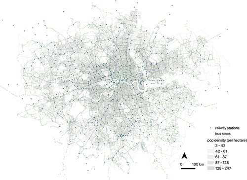
This study utilizes a case study from London to demonstrate a measure of spatial resilience and analysis of recovery. London is a monocentric city (Cox, Prager, and Rose 2011) with spatial patterns in travel mode choice. The primary mode of transport in Inner London is public transport, whereas outer London has a higher share of the private car usage (Cox, Prager, and Rose 2011; TfL 2020d). Figure 2 demonstrates the monocentric nature of London, which concentrates population and resources within the central region, increasing its vulnerability to significant disruptions (Lu et al. 2021).

Figure 2. Map of London railway stations and bus stations.

A map of London railway stations and bus stops relative to the population density within London. Railway stations are in blue, and bus stops are in green. The population density in gray represents the monocentric distribution of London’s residents.

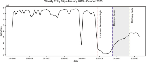
On 23^rd, March 2020, the UK government announced that people should not travel unless for essential reasons to prevent the spread of COVID-19. Figure 3 demonstrates the trend of weekly entries at both railway stations and bus stops from January 2019 to October 2020. The month of May 2020 is artificially low as data on bus boardings was not captured when fare revenue collection paused for buses (TfL 2020d). The recovery horizon to be analyzed starts at the second week of June, when schools have reopened and ridership data reflect levels similar to the week lockdown restrictions began. The analysis horizon ends with the week of 7^th, September, the week before the “rule of six” was implemented – where gatherings could only contain a maximum of six people (UK Home Office 2020). Figure 3 depicts the analysis horizon against weekly trips.

Figure 3. Trend of total weekly entries.

Red dotted line is 23^rd March 2020, when restrictions were first imposed. Blue dotted lines indicate the horizon of recovery to be analyzed: from 8^th June 2020 to 7^th September 2020.

3.1. Data

For this analysis, spatial resilience is measured as the slope of recovery of public transport demand within each Middle Layer Super Output Area (MSOA) in London. MSOAs are census boundaries designed to represent the most equal population size (approximately 9,100 residents per MSOA in London, 982 MSOAs total) and homogeneity of socio-economic status and spatial compactness (Harris 2020). The resilience measure is based on rail passenger ridership data (TfL 2020a, 2020b), and bus alighting data are received from a freedom of information data request to TfL. Data only represents the count of daily entries. To maintain anonymity in the data, certain bus stops with a count of less than five daily entries are reported as “<5”. For this analysis, all less than 5 daily trips are assumed to be the minimum value of one.

Spatial attributes selected for this analysis include categories of socioeconomic data, build environment, and the risk perception of transmitting COVID-19 (as represented by COVID-19 death rate). These are detailed in Table 2, including the source, and existing literature that supports the hypothesis that these features may explain variance in the resilience measure. All features are sourced from spatial datasets and are aggregated at the MSOA level.

Table 2. Explanatory features used in this analysis.

Category	Feature	Label	Description & year	Source of Data
Socioeconomic	IMD score	imd_score	Index of multiple deprivation. A lower score indicates less deprived populations. (2019)	(University of Sheffield 2021)
	Homeworking percent	hw_pct	The ONS homeworking survey indicates level of homeworking by industry (2020). This is applied to Census 2011‘s information of jobs at a MSOA level.	(ONS 2020, 2013)
	Total income	total_income	Annual household income by MSOA. (2015/2016)	(ONS 2015)
	Cars per household	cars_per_hhld	Average number of cars per household by MSOA. (2011)	(GLA 2014)
Built Environment	Cycle length per hectare	cyclelength_perhect	Metres of cycling lanes from TfL’s cycling infrastructure data per hectare by MSOA. (2020)	(TfL 2019)
	Road length per hectare	roadlength_perhect	Metres of road per hectare by MSOA. (2021)	(OS 2021)
	Density of educational spaces	education_den	Density of education locations by MSOA, including primary, second, and tertiary (2021)	(OS 2020)
	Density of public transport infrastructure	pubtrans_den	Density of public transport infrastructure by MSOA. Inclusive of rail stations, bus stops, bus depots, and garages. (2021)
	Density of recreational spaces	recreation_den	Density of recreational spaces by MSOA. (2021)
Risk Perception	Density of COVID deaths	coviddeaths_den	Density of deaths from COVID-19 by MSOA. (2020)	(ONS 2021)

These variables are selected based on the assumption that the spatial attributes of where a trip starts influence the demand for public transport. The provided ridership data only indicate daily entry counts at each station, not capturing where the journey ended or purpose (i.e. workplace, school, and return to home). This analysis assumes that explanatory features may impact public transport demand recovery despite an inability to distinguish between socioeconomic attributes of passengers and destinations that incentivize travel.

4. Methodology

The study follows a straightforward workflow to determine the factors that influence the spatial resilience of public transport demand. The workflow is composed of two primary steps: (1) an estimated resilience measure based on counterfactual demand and (2) a spatial analysis of this resilience measure to determine explanatory features at a global and local level.

4.1. Resilience measure

To estimate the counterfactual demand scenario – estimated demand had the pandemic not occurred – pre-COVID-19 figures were used as a baseline. The activities in the months of June 2019 to September 2019 are used to estimate the counterfactual demand. This approach mirrors existing mobility indices from Google and Citymapper. These indices compared current travel against the previous year to describe how mobility changed due to COVID-19 (Ghosh 2020; Google 2021).

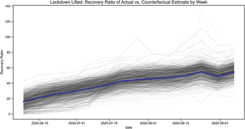
The spatial resilience of public transport demand recovery is defined as the Spatial Resilience Measure (SRM). This analysis defines SRM as the slope of the Recovery Ratio (RR) of actual trips versus counterfactual trips. The ratio (RR) of actual trips versus counterfactual trips is calculated for all zones (e.g. MSOA zones). A linear regression model is fit to the (RR) by week and the resulting slope parameter is the SRM for each MSOA.

Three steps were undertaken to estimate the SRM, detailed as:

1. Calculated the RR for each spatial unit (e.g. MSOA zone).

2. Decomposed the trend of RR by time-series analysis (Perktold, Seabold, and Taylor 2019). In this study of London, the decomposed trend calculates a moving average across periods of 2 weeks. This process yields 10 weeks of data to compute the slope.

3. Fitted a regression to estimate the slope of the decomposed trend line:

$\mathrm{RR}={\alpha }_0+\mathrm{SRM}\mathit{x},$ where $\mathrm{RR}=\frac{\mathrm{Actual}\mathrm{Trips}}{\mathrm{Counter}\mathrm{factual}\mathrm{Trips}}$

where ${\alpha }_0$ is the intercept, $\mathrm{SRM}$ is the slope parameter, and $\mathit{x}$ is the number of weeks. This approach is limited in that it assumes that the slope of a linear model will encapsulate the variation in travel demand recovery. This assumption is explored further in Appendix C.

4.2. Multivariate spatial regression

Once the dependent variable $\mathrm{SRM}$ is calculated, explanatory features are added to the analysis. All features are standardized by utilizing the z-score method. A Variance Inflation Factor (VIF) test is applied to test features for multi-collinearity, strongly correlated features are removed.

A comprehensive analysis is provided by combining results from a global model (i.e. spatial lag model) and a local model (i.e. GWR model). The regression models investigate the hypothesis that the selected explanatory features may significantly explain the spatial variance in the rate of public transport demand recovery. However, there are nuances in each of the models. A spatial lag model assumes a “diffusive” behavior (Sparks and Sparks 2010) in public transport demand. Increased demand in one area is likely to positively influence demand in neighboring areas. The GWR model is a localized approach that allows for an examination of the relationship between the explanatory variables and dependent variables within each defined bandwidth (Fotheringham 2009). This process identifies the contribution of each explanatory variable on each spatial unit.

Table 3 summarizes the baseline OLS model and the global and local spatial regression models utilized. We detail how spatial data is incorporated in the model and the formula for this analysis. All analytical models in this research are developed based on PySAL library (Rey and Anselin 2007).

Table 3. Summary of regression models utilized.

Model	Formula
OLS model	$\mathrm{SRM}={\alpha }_0+\mathit{\beta X}+\mathit{\epsilon }$ Where $\mathrm{SRM}$ is the dependent variable spatial resilience, ${\alpha }_0$ is the intercept, $\mathit{\beta }$ is a vector of parameters for each explanatory feature in vector $\mathit{X}$, and $\mathit{\epsilon }$ is the error term
Spatial lag model	$\mathrm{SRM}={\alpha }_0+\mathit{\beta X}+\mathit{\rho W}\mathrm{SRM}$ Where $\mathit{\rho W}\mathrm{SRM}$ is the spatial lag of dependent variable $\mathrm{SRM}$, $\mathit{\rho }$ is the spatial lag parameter, and $\mathit{W}$ is the spatial weights matrix of $\mathrm{SRM}$.
GWR model	$\mathrm{SR}{\mathrm{M}}_i={\alpha }_{\mathit{i}0}+\sum _{\mathit{k}=1}^K{\beta }_{\mathit{ik}}{X}_{\mathit{ik}}+{ϵ}_i$ Where ${\alpha }_{\mathit{i}0}$ is the intercept coefficient at each location $\mathit{i}$, ${\beta }_{\mathit{ik}}$ is a vector of parameter which is estimated as detailed by: $\widehat{{\beta }_i}={\left[\mathit{X}\prime {\mathit{W}}_i\mathit{X}\right]}^{-1}\mathit{X}\prime {\mathit{W}}_i\mathrm{SRM}$ Where ${\beta }_{\mathit{ik}}$ measures the influence of vector $\mathit{X}$ on the dependent variable $\mathrm{SRM}$ according to the spatial weights matrix ${\mathit{W}}_i$. The bandwidth is selected by optimisation criteria based on the corrected Akaike Information Criterion (AICc) (Oshan et al. 2019)

Through the analysis of the spatial regression model outputs, statistically significant features are identified. The bivariate Moran’s I, a form of spatial correlation, measures the spatial autocorrelation between an explanatory feature and the spatially lagged dependent variable (Anselin 2019). This metric allows for spatial analysis of the relationship between significant features and the dependent variable, $\mathrm{SRM}$.

5. Results

5.1. Spatial resilience of public transport demand

The SRM is the slope of the RR for each MSOA displayed in Figure 4. The methodology detailed in section 4.1 to calculate the spatial resilience measure results for 981 distinct linear regression models. It is found that 75% of these models yield an R-Squared of 0.92 or higher, indicating a strong fit for the majority of the MSOAs. The calculated distribution of the $\mathrm{SRM}$ ranges from 0.24 to 7.91. Therefore, at maximum, an MSOA recovered 7.91% points every week after lockdown restrictions were lifted.

Figure 4. Lockdown lifted: trend of percent actual trips versus counterfactual estimate.

Trend line of actual versus estimated trips over the analysis time horizon. Individual MSOAs are in gray, and the average trend is in blue.

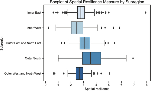
Plotting the SRM reveals spatial heterogeneity – where values vary based on the location in a systematic manner (Sparks and Sparks 2010). The boxplot in Figure 5 segments the SRM by subregion. Immediately, two interesting patterns appear: much of the Inner West of London (e.g. Camden, Kensington & Chelsea, and Hammersmith & Fulham) and Outer West (e.g. Brent) has low spatial resilience, whereas much of South London (e.g. Sutton and Merton) has relatively higher spatial resilience. Inner London has a mean spatial resilience of 2.74, whereas outer London has a mean spatial resilience of 3.10. This finding aligns with previous research that Outer London is recovering faster than Inner London (TfL 2020d). Further definition of categorized MSOA regions is given in Appendix A, B and C.

Figure 5. Boxplot of SRM by subregion.

MSOAs are divided by inner and outer regions. MSOAs in the Inner East and Inner West have lower spatial resilience than Outer MSOAs, although Outer West and North West are more similar to Inner MSOAs.

The visual observation of spatial dependency can be validated through a calculation of statistical significance, the global Moran’s I. The global Moran’s I value is 0.39, indicating a small amount of positive spatial correlation. This value is estimated to be statistically significant against a randomized dataset with a p-value of 0.001.

The Local Indicator of Spatial Association (LISA) gives a statistic for each location with an assessment of significance (Anselin 1995). It is applied here to identify which MSOAs have a significant spatial relationship with the resilience measure. Following Rey, Arribas-Bel, and Wolf’s (2020) method, MSOAs were clustered based on their values relative to the average spatial resilience. Figure 6 spatially plots the statistically significant values. The LISA statistics identifies areas where there may be spatial features influencing the observed spatial autocorrelation.

Figure 6. LISA.

The LISA spatial plot includes only those MSOAs that have statistically significant clustering.

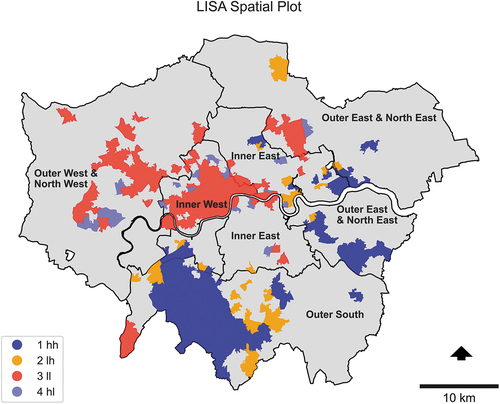
Figure 6 plots each statistically significant LISA values and categorizes them into four clusters: high–high (“hh”), low–high (“lh”), low–low (“ll”), and high–low (“hl”). This clustering draws interest into the commonality between high performing and low performing MSOAs to produce these spatial patterns. High–high and low–low clusters are regions that, respectively, have a higher-than-average or lower-than-average spatial resilience surrounded by similar regions. High–low clusters are areas with high rates surrounded by low spatial resilience, whereas low–high clusters are areas with low spatial resilience surrounded by high spatial resilience (Rey, Arribas-Bel, and Wolf 2020; Sparks and Sparks 2010). MSOAs within Merton and Sutton local authorities in Southwest London belong to the high–high clusters, whereas MSOAs in the Inner West and Inner East of London are in the low–low clusters.

This process of estimating the SRM and its Moran’s I confirm this paper’s hypothesis that there is spatial dependency in the recovery of public transport demand. It warrants an investigation into the spatial attributes that may contribute to high or low resilience within different areas of London. They are detailed in the following section.

5.2. Spatial socioeconomic factors contributing to spatial resilience

The features of socioeconomic indicators, built environment, and risk perception are standardized and tested for multicollinearity prior to modeling. Table 4 details the performance of the three regression models.

Table 4. Summary of regression models.

	OLS		Spatial lag		GWR
Statistics	coefficient	P > |t|	coefficient	P > |t|	coefficient (mean)	range
constant	0.00	1.00	−0.01	0.77	0.02	(−0.51, 0.73)
total_income_std	−0.18	0.00	−0.17	0.00	−0.22	(−0.51, 0.09)
hw_pct_std	−0.01	0.92	0.04	0.47	0.00	(−0.33, 0.41)
cyclelength_std	0.00	0.90	0.00	0.99	−0.01	(−0.32, 0.16)
carsperhhld_std	0.27	0.00	0.14	0.05	0.33	(0.11, 0.79)
roadlengths_std	−0.01	0.77	0.02	0.58	−0.01	(−0.15, 0.28)
education_den_std	0.05	0.37	0.07	0.15	0.15	(−0.27, 0.75)
pubtrans_den_std	−0.08	0.09	−0.09	0.04	−0.44	(−2.85, 0.24)
recreation_den_std	−0.04	0.44	−0.01	0.74	0.02	(−0.31, 0.30)
coviddeaths_den_std	−0.01	0.70	−0.03	0.31	0.01	(−0.15, 0.28)
spatial_lag_SRM			0.62	0.03
R-Squared	0.08		0.33		0.35*
AIC	2720.13		2422.66*		2511.25
Moran’s I of residuals	0.35		−0.05		0.13

Variables that are statistically significant are in bold. Furthermore, the model with the highest R-Squared and lowest AIC are indicated by *. The bandwidth selected for the GWR model is 333.

The R-squared value, AIC, and Moran’s I of residuals are compared to assess the performance of the regression models. The baseline OLS model explains only 8% of the variation in spatial resilience. The spatial lag model and GWR improve on this value, with the GWR model explaining the highest amount of variance at 35%. The AIC is another metric for goodness of fit, where a lower value indicates a stronger fit (Fotheringham 2009). Furthermore, the Moran’s I of the residuals determines whether spatial autocorrelation is still present in the data or if it has been explained by the model. The spatial lag model successfully reduces the global Moran’s I to −0.05 and the GWR reduces it to 0.13.

These results support the conclusions of spatial dependency within the data. The model with the lowest AIC – the spatial lag model – indicates that the SRM is influenced by neighboring regions. Therefore, an increase in public transport demand in one MSOA is likely to similarly appear in neighboring regions. Although the GWR model has a higher AIC score than the spatial lag model, its higher R-squared justifies a localized analysis of the significant features. As the variables are standardized, a one-unit change in the explanatory feature is equivalent to a one standard deviation change in that feature (Taboga 2017). For each feature, a positive coefficient indicates a positive association with the $\mathrm{SRM}$ whereas a negative coefficient indicates a decrease in the $\mathrm{SRM}$.

Across the models, features of total income, cars per household, and public transport infrastructure density have a p-value less than or equal to 0.05, implying statistical significance for the variance in spatial resilience. The main feature for risk perception, COVID-19 deaths density, does not appear to be statistically significant. In the context of this modeling, COVID-19 death rates within the specific MSOA do not significantly influence public transport demand. Due to the limited testing at the beginning of the pandemic, the death density metric was selected instead of case numbers as it is a more accurate depiction of COVID-19 spread. However, the lack of statistically significant influence could be impacted by the absence of a temporal element in the models. There is a time delay between infection and death, and a model that includes these temporal impacts may better demonstrate the weekly influence on public transport demand. Furthermore, it may also be possible that a higher aggregation (i.e. London or the UK) may have an influence on local public transport behaviors.

The GWR model depicts a spatially heterogeneous relationship between total income and public transport infrastructure density with $\mathrm{SRM}$. In the case of total income, its parameter estimates range from −0.51 to 0.09. This finding implies that there is a dependency on the location of the relationship with $\mathrm{SRM}$. That is, an increase in total income may either reduce or increase the spatial resilience of public transport demand. For the public transport infrastructure density variable, the parameter estimates range from −2.85 to 0.24, implying a similar spatially dependent relationship as the total income feature. Therefore, it is important to explore the localized relationship of these variables with $\mathrm{SRM}$.

Figure 7. Bivariate analysis of most significant features.

Plot of spatial resilience measure and top three significant features based on bivariate Moran’s I. Similar to before, each MSOA has been categorized into high–high, low–high, low–low, and high–low clusters. For example, from the total income plot, a low–high cluster indicates an area with less than average income level in an area that is above the average spatial resilience.

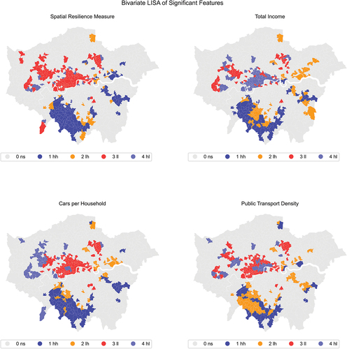
Globally, total income has a negative relationship with the spatial resilience measure, although the relationship is more nuanced at a local level. In Figure 7, a high total income in Inner London directly corresponds with the low spatial resilience, aligning with the global relationship. However, in the Outer South of London, high income is also present in high areas of recovery. Counterintuitively, $\mathrm{SRM}$ has a positive relationship with cars per household and a negative relationship with public transport density. This appears to imply a decoupled relationship where areas continue to use public transport despite high car ownership and low density of public transport infrastructure. There is also a varied relationship between public transport density and spatial resilience. Within Inner London, areas that have high public transport infrastructure density have low spatial resilience. However, there are also areas with low public transport infrastructure density and low spatial resilience.

To provide context for the above findings, further analysis of the difference in journey purposes between areas with high cars per household or high public transport infrastructure density is needed. As discussed previously, the data does not distinguish between attributes of the origin of a journey versus the points of interest that may influence a journey’s destination. Without a transparent linkage between rider’s sociodemographic attributes and their chosen destinations, it is challenging to definitively draw a conclusion of the influences on spatial resilience.

5.3. Policy recommendations

5.3.1. Data collection of homeworking behavior

Whilst the homeworking feature was not statistically significant, it had a high correlation with total income (0.83) and the total income’s VIF (4.31) was close to the VIF threshold of 5. Therefore, models that utilize homeworking percentage instead of total income are likely to find that homeworking is statistically significant. Research conducted by ONS in April 2021 found that 24% of the businesses expected an increase in homeworking going forward, with 85% of working adults desiring a hybrid approach of both homeworking and office working (Casey 2021). Cox et al.’s investigation of the resilience of the London Underground demand after the 2005 terrorist bombings hypothesized that some journeys may have shifted to telecommuting (Cox, Prager, and Rose 2011). Data that defines homeworking as a trip mode could be collected via the London Travel Demand Survey (LTDS), an annual travel survey of sample households (TfL 2021a). This data can identify whether Londoners are moving toward a “remote revolution” (TfL 2020d). Furthermore, this data will allow for future analysis of transport resilience from an ecological perspective (Modica and Reggiani 2015), providing quantitative evidence of how the public transport demand not just recovers but adapts.

5.3.2. Align services and investments to public transport resilience

The high levels of spatial resilience in Merton and Sutton (Figure 7) reveal an opportunity to reconsider public transport services. Additional research is required to understand the purpose and destination of the public transport trips occurring in Outer London. If demand consistently recovers in the outer south, services may need to initially “right-size” (Dickie et al. 2021) to the reduced commuting in central London. Furthermore, a future investment may be reallocated toward areas that are showing greater resilience in the public transport demand (TfL 2020d). More resilient routes can serve as a baseline for funding negotiations and investments (Campaign for Better Transport 2020), potentially garnering greater support from local authorities. If schemes that enable more localized forms of travel are pursued, it may move London toward a future of low carbon localism (TfL 2020d).

5.3.3. Polycentric future

The spatial heterogeneity in $\mathrm{SRM}$ minimizes global predictability in the behavioral response to public transport policy solutions. A low carbon localized future shifts London away from its current monocentric spatial pattern toward a polycentric design. A polycentric design yields a different level of spatial resilience: one that introduces spatial redundancy through modular infrastructure, multiple sizes of support systems, and a spatially equitable recovery from disruptions (Lu et al. 2021; Münter and Volgmann 2021). Therefore, a polycentric response to public transport demand may reduce the spatial heterogeneity observed in the $\mathrm{SRM}$. Policies that support a polycentric future may enhance the resilience of localized public transport demand and will require a balance in resources and land use planning to offset potential harms (Lu et al. 2021).

6. Conclusion and discussion

This research contributed a spatial resilience perspective to the discussion of post-pandemic urban mobility. Spatial resilience relates spatial attributes to the resilience of the studied system, allowing for an analysis of factors that influence spatial heterogeneous behavior in recovery. Specifically, $\mathrm{SRM}$ is defined as the slope of the RR of actual trips versus counterfactual trips. This measure is applied to a case study of London public transport. For 75% of the MSOAs, a linear model resulted in a strong R-squared value above 0.92, indicating that a linear model is a good estimator of the slope of the RR. However, a future analysis should consider non-parametric methods such as Thein-Sen to estimate the slope for MSOAs with non-linear behavior (Hussain and Mahmud 2019).

London’s spatial differences in public transport recovery after the first lockdown restrictions were analyzed. Through comparison of the spatial resilience of public transport demand across MSOAs, this research identified pathways to recovery. The significant features of income, car ownership, and public transport density were shown to have global significance. Therefore, despite the lack of data on an individual’s trip destination or purpose, it was still possible to find significant spatial influences on the $\mathrm{SRM}$. Among the variables of income and public transport density, spatially varying relationships invite further research into individuals’ behaviors and trip purposes.

The spatial resilience heterogeneity influenced by these spatial attributes may result in a comprehensive review of the public transport service provision in the future. The consistent and continuous monitoring of the spatial recovery and influential attributes including homeworking behavior will inform decisions and provide evidence to shape the “new normal” of London. This “new normal” will need to allow for a diversity of travel purposes whilst correcting for existing inequities.

Despite the relatively improved performance of the spatial regression models versus OLS, the base model only explains 8% of the variance. This indicates an opportunity for refinement in the data inputs and additional features to improve the baseline modeling. Data that distinguishes the origin versus destination and additional research of trip purpose could improve the fit. Detailed and long-term public transport demand data such as bus route-level journey counts and rail station and train usage data (TfL 2020c) may provide more insight into where trips are recovering relative to points of interest. Furthermore, the forthcoming census 2021 may provide a more accurate and up-to-date representation of socioeconomic attributes that have spatial dependencies with the resilience of public transport demand.

This methodology could be applied to the recovery after the second lockdown to determine whether the trends in this research are consistent. The zones utilized for this analysis are vulnerable to the Modifiable Areal Unit Problem (MAUP), where the model results are likely to be sensitive to varying definitions of zones (Fotheringham and Wong 1991; Young et al. 2021). Therefore, conducting this same analysis at different levels of aggregation may help determine whether the findings are consistent (Fotheringham and Wong 1991). Future work should return to Bešinović’s resilience model (2020) (Figure 1) and analyze each stage of the triangle of ridership recovery and identify the influential spatial features of a region’s robustness and recovery from the effects of the COVID-19 pandemic.

Data available statement

The data that support the findings of this study are openly available on GitHub at https://github.com/divyasharma-git/spatial-resilience. The raw data (i.e. bus and tube gate counts) can be made available from Transport for London upon reasonable request via FOI.

Disclosure statement

No potential conflict of interest was reported by the authors.

Additional information

Funding

This project has received funding from the European Research Council (ERC) under the European Union’s Horizon 2020 research and innovation programme (grant agreement No 949670), and from ESRC under JPI Urban Europe/NSFC (grant No. ES/T000287/1). We thank Transport for London (TfL) sincerely for their support of COVID-related research.

Notes on contributors

Divya Sharma

Divya Sharma received her MSc degree in Smart Cities and Urban Analytics from UCL in 2021 and an MPhil in Sustainable Development from Cambridge University in 2020. Her research interests include equitable transport decarbonization solutions and spatial analytics.

Chen Zhong

Chen Zhong Associate Professor in Urban Analytics at the Bartlett Centre for Advanced Spatial Analysis (CASA), UCL. Her research interests include spatial data mining, spatial network analysis, and the use of such analytical techniques for urban and transport planning.

Howard Wong

Howard Wong is a Principal Transport Planner in Transport for London, and he is currently doing a part-time PhD at Centre of Advance Spatial Analysis (CASA) in University College London (UCL). His work and study focus on mobility data, particularly on areas such as connectivity, public transport provision, travel behavior and spatial analysis.

Appendices Appendix A.

Categorisation of Local Authorities to Subregion

Table

Region	Subregion	Local authority
Inner	Inner East	Hackney
		Haringey
		Islington
		Lambeth
		Lewisham
		Newham
		Southwark
		Tower Hamlets
	Inner West	Camden
		City of London
		Hammersmith and Fulham
		Kensington and Chelsea
		Wandsworth
		Westminster
Outer	Outer East and North East	Barking and Dagenham
		Bexley
		Enfield
		Greenwich
		Havering
		Redbridge
		Waltham Forest
	Outer South	Bromley
		Croydon
		Kingston upon Thames
		Merton
		Sutton
	Outer West and North West	Barnet
		Brent
		Ealing
		Harrow
		Hillingdon
		Hounslow
		Richmond upon Thames

Appendix B.

Modelling parameters

Time-series method to calculate the slope of the RR:

The decomposition method utilized the python package statistical model and applied the function seasonal decomposition (Perktold, Seabold, and Taylor 2022). This is a seasonal decomposition using moving averages. The decomposition model assumed a linear behavior in the underlying dataset and applied an additive model. The time-series dataset is 14 weeks of data and assumes a period of 2 weeks – thereby calculating the moving average of 2 weeks at a time.

GWR model:

The kernel size and bandwidth for the GWR model were selected by utilizing the Sel_BW class within the python mgwr package (Oshan et al. 2019). Oshan et al. (2019) provide the following guidance for kernel functions: A kernel set to bisquare ensures observations greater than the number of nearest neighbors from the calibration location have no influence. Gaussian and exponential kernel functions allow all observations to have a non-zero weight from the calibration location regardless of distance. Therefore, a bisquare function is selected to limit the influences on neighboring datapoints. Furthermore, the kernel type is set to adaptive, which allows for the study of irregular shaped areas or non-uniform spatial distributions. The bandwidth is selected by utilizing a golden search optimization with an AICc. Further details of model specification are available in Appendix B.

Appendix C.

Non-parametric modelling for the RR

Linear regression method

To calculate the slope of the RR for each MSOA, a linear regression model was utilized. This is a simple method that assumes linear behavior in the underlying data. In this case, the underlying data is the decomposed trend of each MSOA. The R-squared was calculated on the residuals for each MSOA, and the descriptive statistics and histogram of this R-squared value is provided in Figure C1.

Table

	min	25%	50%	75%	max
R-Squared	0.075	0.923	0.961	0.982	0.999

Figure C1. Histogram of R-Squared for all linear regression models.

This histogram provides the R-squared for every linear regression model utilized to calculate the slope of the RR.

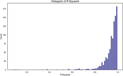
It is found that at least 75% of the calculated 981 linear regression models have an R-squared value of 0.92 or above. This implies that a linear regression model is a strong fit for the majority of the datapoints. For the 25% of the regression models that do not have a high R-squared value, a non-parametric method may be an appropriate estimator.

Mann–Kendall test & Thein–Sen slope

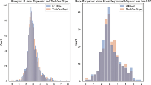
The Mann–Kendall test is a statistic that identifies the trend without the requirement of linear data. It does, however, require that the underlying data not be serially correlated over time. In this case, the RR for each week contains autocorrelation. Therefore, a modified Mann–Kendall test, Hamed–Rao, is applied instead. This test accounts for autocorrelation within the data. The python pyMannKendall package is utilized for this analysis (Hussain and Mahmud 2019). First, it is found that 977 out of 981 MSOAs have an increasing trend. Second, it is found that the Thein-Sen slope estimator provides a fairly similar distribution in slope estimates overall. Figure C2 compares the distribution of slope estimates for all 981 MSOAs against those where the linear regression model had an R-squared less than 0.92, the Thein–Sen slope estimator recommends a lower slope value. This non-parametric may be a potential improvement for the MSOAs that demonstrate non-linear behavior.

Figure C2. Histogram of linear regression slope and Theil–Sen Slope estimator.

The full dataset versus those where the linear regression R-squared was less than 0.92. The histogram on the left compares the two slope estimators across the entire dataset. The distributions are largely similar. The histogram on the right compares the two slope estimators where the linear regression R-squared is less than 0.92. The distributions are still similar, although the Theil–Sen slope estimator has a slightly smoother distribution for slope estimates between 2 and 4.

References

- Abdullah, M., C. Dias, D. Muley, and M. Shahin. 2020. “Exploring the Impacts of COVID-19 on Travel Behavior and Mode Preferences.” Transportation Research Interdisciplinary Perspectives 8 (November): 100255. doi:10.1016/j.trip.2020.100255.
- Allen, C. R., D. G. Angeler, G. S. Cumming, C. Folke, D. Twidwell, and D. R. Uden. 2016. ”Quantifying Spatial Resilience.” Edited by Joseph Bennett. The Journal of Applied Ecology 53 (3): 625–635. doi:10.1111/1365-2664.12634.
- Anselin, L. 1995. “Local Indicators of Spatial Association-LISA.” Geographical Analysis 27 (2): 93–115. doi:10.1111/j.1538-4632.1995.tb00338.x.
- Anselin, L. 2019. “Global Spatial Autocorrelation (2).” https://geodacenter.github.io/workbook/5b_global_adv/lab5b.html#bivariate-spatial-correlation—a-word-of-caution
- Azolin, L. G., A. N. R. da Silva, and N. Pinto. 2020. “Incorporating Public Transport in a Methodology for Assessing Resilience in Urban Mobility.” Transportation Research Part D: Transport and Environment 85 (August): 102386. doi:10.1016/j.trd.2020.102386.
- Barbieri, D. M., B. Lou, M. Passavanti, C. Hui, I. Hoff, D. A. Lessa, G. Sikka, et al. 2021. ”Impact of COVID-19 Pandemic on Mobility in Ten Countries and Associated Perceived Risk for All Transport Modes.” PLoS One 16 (2): e0245886. doi:10.1371/journal.pone.0245886.
- Basu, R., and J. Ferreira. 2021. “Sustainable Mobility in Auto-Dominated Metro Boston: Challenges and Opportunities Post-COVID-19.” Transport Policy 103 (March): 197–210. doi:10.1016/j.tranpol.2021.01.006.
- Batty, M., R. Murcio, I. Iacopini, M. Vanhoof, and R. Milton. 2020. ”London in Lockdown: Mobility in the Pandemic City.” 19. doi:10.48550/arXiv.2011.07165.
- Bešinović, N. 2020. “Resilience in Railway Transport Systems: A Literature Review and Research Agenda.” Transport Reviews 40 (4): 457–478. doi:10.1080/01441647.2020.1728419.
- Bruneau, M., S. E. Chang, R. T. Eguchi, G. C. Lee, T. D. O’Rourke, A. M. Reinhorn, M. Shinozuka, K. Tierney, W. A. Wallace, and D. von Winterfeldt. 2003. “A Framework to Quantitatively Assess and Enhance the Seismic Resilience of Communities.” Earthquake Spectra 19 (4): 733–752. doi:10.1193/1.1623497.
- Campaign for Better Transport. 2020. “Covid-19 Recovery: Renewing the Transport System.” https://bettertransport.org.uk/wp-content/uploads/legacy-files/research-files/Covid_19_Recovery_Renewing_the_Transport_System.pdf
- Casey, A. 2021. “Business and Individual Attitudes Towards the Future of Homeworking, UK - Office for National Statistics.” https://www.ons.gov.uk/employmentandlabourmarket/peopleinwork/employmentandemployeetypes/articles/businessandindividualattitudestowardsthefutureofhomeworkinguk/apriltomay2021
- Chen, Y., M. Chen, B. Huang, C. Wu, and W. Shi. 2021. “Modeling the Spatiotemporal Association Between COVID-19 Transmission and Population Mobility Using Geographically and Temporally Weighted Regression.” GeoHealth 5 (5): e2021GH000402. doi:10.1029/2021GH000402.
- Christidis, P., A. Christodoulou, E. Navajas-Cawood, and B. Ciuffo. 2021. “The Post-Pandemic Recovery of Transport Activity: Emerging Mobility Patterns and Repercussions on Future Evolution.” Sustainability 13 (11): 6359. doi:10.3390/su13116359.
- Ciuffini, F., S. Tengattini, and A. Y. Bigazzi. 2021. ”Mitigating Increased Driving After the COVID-19 Pandemic: An Analysis on Mode Share, Travel Demand, and Public Transport Capacity.” Transportation Research Record: Journal of the Transportation Research Board, no. August: 036119812110378. doi:10.1177/03611981211037884.
- Cox, A., F. Prager, and A. Rose. 2011. “Transportation Security and the Role of Resilience: A Foundation for Operational Metrics.” Transport Policy 18 (2): 307–317. doi:10.1016/j.tranpol.2010.09.004.
- Dickie, J., A. Tyndall, R. de Cani, A. Nothstine, D. Philips, and P. Andison. 2021. “Transport in London: New Solutions for a Changing City.” https://www.businessldn.co.uk/sites/default/files/documents/2021-01/TransportInLondon.pdf
- D’Lima, M., and F. Medda. 2015. “A New Measure of Resilience: An Application to the London Underground.” Transportation Research Part A: Policy and Practice 81 (November): 35–46. doi:10.1016/j.tra.2015.05.017.
- Fotheringham, A. S. 2009. “Geographically Weighted Regression.” In The SAGE Handbook of Spatial Analysis, edited by A. Fotheringham and P. Rogerson, 242–253. London, UK: SAGE Publications, Ltd. doi:10.4135/9780857020130.n13.
- Fotheringham, A. S., and D. W. S. Wong. 1991. “The Modifiable Areal Unit Problem in Multivariate Statistical Analysis.” Environment and Planning A: Economy and Space 23 (7): 1025–1044. doi:10.1068/a231025.
- Ghosh, I. 2020. “Global Shutdown: Visualizing Commuter Activity in the World’s Cities.” Visual Capitalist, March 27. https://www.visualcapitalist.com/covid-19-cities-commuter-activity/
- GLA (Greater London Authority). 2014. “MSOA Atlas - London Datastore, Electronic Dataset.” https://data.london.gov.uk/dataset/msoa-atlas
- Google. 2021. “COVID-19 Community Mobility Report.” COVID-19 Community Mobility Report. https://www.google.com/covid19/mobility?hl=en
- Harris, R. 2020. “Exploring the Neighbourhood-Level Correlates of Covid-19 Deaths in London Using a Difference Across Spatial Boundaries Method.” Health & Place 66 (November): 102446. doi:10.1016/j.healthplace.2020.102446.
- Holling, C. S. 1973. “Resilience and Stability of Ecological Systems.” Annual Review of Ecology and Systematics 4 (1): 1–23. doi:10.1146/annurev.es.04.110173.000245.
- Huang, X., Z. Li, Y. Jiang, X. Ye, C. Deng, J. Zhang, and X. Li. 2021. “The Characteristics of Multi-Source Mobility Datasets and How They Reveal the Luxury Nature of Social Distancing in the U.S. During the COVID-19 Pandemic.” International Journal of Digital Earth 14 (4): 424–442. doi:10.1080/17538947.2021.1886358.
- Hussain, M., and I. Mahmud. 2019. “Pymannkendall: A Python Package for Non-Parametric Mann-Kendall Family of Trend Tests.” OS Independent. Python. https://github.com/mmhs013/pymannkendall
- Jiang, P., X. Fu, Y. Van Fan, J. J. Klemeš, P. Chen, S. Ma, and W. Zhang. 2021. “Spatial-Temporal Potential Exposure Risk Analytics and Urban Sustainability Impacts Related to COVID-19 Mitigation: A Perspective from Car Mobility Behaviour.” Journal of Cleaner Production 279 (January): 123673. doi:10.1016/j.jclepro.2020.123673.
- Lu, Y., G. Zhai, S. Zhou, and Y. Shi. 2021. “Risk Reduction Through Urban Spatial Resilience: A Theoretical Framework.” Human and Ecological Risk Assessment: An International Journal 27 (4): 921–937. doi:10.1080/10807039.2020.1788918.
- Ma, X., J. Yanjie, Y. Jin, J. Wang, and H. Mingjia. 2018. “Modeling the Factors Influencing the Activity Spaces of Bikeshare Around Metro Stations: A Spatial Regression Model.” https://www.mdpi.com/2071-1050/10/11/3949/htm
- Modica, M., and A. Reggiani. 2015. “Spatial Economic Resilience: Overview and Perspectives.” Networks & Spatial Economics 15 (2): 211–233. doi:10.1007/s11067-014-9261-7.
- Münter, A., and K. Volgmann. 2021. “Polycentric Regions: Proposals for a New Typology and Terminology.” Urban Studies 58 (4): 677–695. doi:10.1177/0042098020931695.
- ONS (Office for National Statistics). 2013. “DC6604EW (Occupation by Industry) - Nomis - Official Labour Market Statistics, Electronic Dataset.” http://www.nomisweb.co.uk/census/2011/dc6604ew
- ONS (Office for National Statistics). 2015. “ONS Model-Based Income Estimates, MSOA - London Datastore, Electronic Dataset.” https://data.london.gov.uk/dataset/ons-model-based-income-estimates–msoa
- ONS (Office for National Statistics). 2020. “Homeworking - Office for National Statistics, Electronic Dataset.” https://www.ons.gov.uk/employmentandlabourmarket/peopleinwork/employmentandemployeetypes/datasets/homeworking
- ONS (Office for National Statistics). 2021. “Deaths Due to COVID-19 by Local Area and Deprivation - Office for National Statistics, Electronic Dataset.” https://www.ons.gov.uk/peoplepopulationandcommunity/birthsdeathsandmarriages/deaths/datasets/deathsduetocovid19bylocalareaanddeprivation
- Oshan, T. M., Z. Li, W. Kang, L. J. Wolf, and A. S. Fotheringham. 2019. “Mgwr: A Python Implementation of Multiscale Geographically Weighted Regression for Investigating Process Spatial Heterogeneity and Scale.” ISPRS International Journal of Geo-Information 8 (6): 269. doi:10.3390/ijgi8060269.
- OS (Ordnance Survey). 2020. “Points of Interest, Electronic Dataset.” https://digimap.edina.ac.uk/webhelp/os/data_information/os_products/points_of_interest.htm
- OS (Ordnance Survey). 2021. “OS Open Roads, Electronic Dataset.” https://osdatahub.os.uk/downloads/open/OpenRoads?_ga=2.106254016.2142301253.1626191853-1483327713.1626191853
- Perktold, J., S. Seabold, and J. Taylor. 2019. “User Guide — Statsmodels.” https://www.statsmodels.org/stable/user-guide.html
- Perktold, J., S. Seabold, and J. Taylor. 2022. “Stats Models Time Series Analysis.” https://www.statsmodels.org/dev/generated/statsmodels.tsa.seasonal.seasonal_decompose.html
- Perrings, C. 1998. “Resilience in the Dynamics of Economy-Environment Systems.” 18.
- Rey, S. J., and L. Anselin. 2007. “PySal: A Python Library of Spatial Analytical Methods.” https://pysal.org/esda/notebooks/spatialautocorrelation.html
- Rey, S. J., D. Arribas-Bel, and L. J. Wolf. 2020. “Geographic Data Science with Python.” https://geographicdata.science/book/intro_part_ii.html
- Rothengatter, W., J. Zhang, Y. Hayashi, A. Nosach, K. Wang, and T. Hoon Oum. 2021. “Pandemic Waves and the Time After Covid-19 – Consequences for the Transport Sector.” Transport Policy 110 (September): 225–237. doi:10.1016/j.tranpol.2021.06.003.
- Saberi, M., M. Ghamami, Y. Gu, M. H. Shojaei, and E. Fishman. 2018. “Understanding the Impacts of a Public Transit Disruption on Bicycle Sharing Mobility Patterns: A Case of Tube Strike in London.” Journal of Transport Geography 66 (January): 154–166. doi:10.1016/j.jtrangeo.2017.11.018.
- Sannigrahi, S., F. Pilla, B. Basu, A. Sarkar Basu, and A. Molter. 2020. “Examining the Association Between Socio-Demographic Composition and COVID-19 Fatalities in the European Region Using Spatial Regression Approach.” Sustainable Cities and Society 62 (November): 102418. doi:10.1016/j.scs.2020.102418.
- Saunders, A., A. Barron, R. Anderson, R. Allport, and D. Mundy. 2021. “COVID-19 Discussion Paper.” 10.
- Smeds, E., J. McArthur, and R. S. Ray. 2020. “Coronavirus Showed the Way Cities Fund Public Transport is Broken – Here’s How It Needs to Change.” The Conversation. http://theconversation.com/coronavirus-showed-the-way-cities-fund-public-transport-is-broken-heres-how-it-needs-to-change-145136.
- Sparks, P. J., and C. S. Sparks. 2010. “An Application of Spatially Autoregressive Models to the Study of US County Mortality Rates: An Application of Spatially Autoregressive Models.” Population, Space and Place 16 (6): 465–481. doi:10.1002/psp.564.
- Taboga, M. 2017. “Linear Regression with Standardized Variables.” https://www.statlect.com/fundamentals-of-statistics/linear-regression-with-standardized-variables
- TfL. 2020a. “Intro to NUMBAT.” crowding.data.tfl.gov.uk/NUMBAT/Intro_to_NUMBAT.pdf
- TfL. 2020b. “Travel in London Report 13.” 264.
- TfL. 2021a. “Consultations & Surveys.” Transport for London. https://www.tfl.gov.uk/corporate/about-tfl/how-we-work/planning-for-the-future/consultations-and-surveys
- TfL. 2021b. “Financial Sustainability Plan - 11 January 2021.” 116.
- TfL Press Office. 2020. “TfL Press Release - Transport for London to Place 7,000 Staff on Furlough to Help Safeguard Vital Transport Services and Support London Through the Coronavirus Pandemic.” https://tfl-newsroom.prgloo.com/news/tfl-press-release-transport-for-london-to-place-7-000-staff-on-furlough-to-help-safeguard-vital-transport-services-and-support-london-through-the-coronavirus-pandemic
- TfL (Transport for London). 2019. “Cycling Infrastructure Database - London Datastore.” https://data.london.gov.uk/dataset/cycling-infrastructure-database
- TfL (Transport for London). 2020c. “FOI Request Detail: Daily Gateline Statistics 2015-2020, Electronic Dataset.” Transport for London. https://www.tfl.gov.uk/corporate/transparency/freedom-of-information/foi-request-detail
- TfL (Transport for London). 2020d. “FOI Request Detail: Station Usage Figures.” Transport for London. https://www.tfl.gov.uk/corporate/transparency/freedom--of-information/foi-request-detail
- TSC. 2021. “COVID-19 Cross Group Benchmarking: Review of Recent Activities.” 17.
- Twumasi-Boakye, R., and J. Sobanjo. 2019. “Civil Infrastructure Resilience: State-Of-The-Art on Transportation Network Systems.” Transportmetrica A: Transport Science 15 (2): 455–484. doi:10.1080/23249935.2018.1504832.
- UK Home Office. 2020. “Rule of Six Comes into Effect to Tackle Coronavirus.” GOV.UK. https://www.gov.uk/government/news/rule-of-six-comes-into-effect-to-tackle-coronavirus
- University of Sheffield. 2021. “IMD2019 - About the Maps, Electronic Dataset.” Electronic dataset. MySociety Research. http://127.0.0.1:8000/sites/imd2019/about/
- Van Audenhove, F. J. 2020. “The Future of Mobility Post-COVID-19.” 40.
- Vickerman, R. 2021. “Will Covid-19 Put the Public Back in Public Transport? A UK Perspective.” Transport Policy 103 (March): 95–102. doi:10.1016/j.tranpol.2021.01.005.
- Wielechowski, M., K. Czech, and Ł. Grzęda. 2020. “Decline in Mobility: Public Transport in Poland in the Time of the COVID-19 Pandemic.” Economies 8 (4): 78. doi:10.3390/economies8040078.
- Young, S. G., J. Datta, B. Kar, X. Huang, M. D. Williamson, J. A. Tullis, and J. Cothren. 2021. “Challenges and Limitations of Geospatial Data and Analyses in the Context of COVID-19.” In Mapping COVID-19 in Space and Time: Understanding the Spatial and Temporal Dynamics of a Global Pandemic, edited by S.-L. Shaw and D. Sui, 137–167. Human Dynamics in Smart Cities. Cham: Springer International Publishing. doi:10.1007/978-3-030-72808-3_8.
- Zhu, Y., K. Xie, K. Ozbay, F. Zuo, and H. Yang. 2017. “Data-Driven Spatial Modeling for Quantifying Networkwide Resilience in the Aftermath of Hurricanes Irene and Sandy.” Transportation Research Record: Journal of the Transportation Research Board 2604 (1): 9–18. doi:10.3141/2604-02.