Fully automatic DOM generation method based on optical flow field dense image matching

ABSTRACT

Automatic Digital Orthophoto Map (DOM) generation plays an important role in many downstream works such as land use and cover detection, urban planning, and disaster assessment. Existing DOM generation methods can generate promising results but always need ground object filtered DEM generation before otho-rectification; this can consume much time and produce building facade contained results. To address this problem, a pixel-by-pixel digital differential rectification-based automatic DOM generation method is proposed in this paper. Firstly, 3D point clouds with texture are generated by dense image matching based on an optical flow field for a stereo pair of images, respectively. Then, the grayscale of the digital differential rectification image is extracted directly from the point clouds element by element according to the nearest neighbor method for matched points. Subsequently, the elevation is repaired grid-by-grid using the multi-layer Locally Refined B-spline (LR-B) interpolation method with triangular mesh constraint for the point clouds void area, and the grayscale is obtained by the indirect scheme of digital differential rectification to generate the pixel-by-pixel digital differentially rectified image of a single image slice. Finally, a seamline network is automatically searched using a disparity map optimization algorithm, and DOM is smartly mosaicked. The qualitative and quantitative experimental results on three datasets were produced and evaluated, which confirmed the feasibility of the proposed method, and the DOM accuracy can reach 1 Ground Sample Distance (GSD) level. The comparison experiment with the state-of-the-art commercial softwares showed that the proposed method generated DOM has a better visual effect on building boundaries and roof completeness with comparable accuracy and computational efficiency.

KEYWORDS:

• Digital Orthophoto Map (DOM)
• dense image matching based on optical flow field (OFFDIM)
• 3D point clouds with texture
• seamline network
• accuracy

1. Introduction

Digital Orthophoto Map (DOM) is an orthogonal projection image made from aerial-space photographic images through element-by-element orthorectification, radiation correction, and mosaicking, which must meet the geometric accuracy requirements of topographic maps and include the image features. DOM is widely used in these fields such as topographic mapping (Gao et al. 2017), 3D object reconstruction (Cheng et al. 2022), power line inspection (Matikainen et al. 2016), disaster assessment (Zhu et al. 2019), geographical situation monitoring (Zhang et al. 2021), urban planning (Yang et al. 2021; Li et al. 2021; Lee et al. 2021), and natural resource survey (Erickson and Biedenweg 2022) because of their high intuitiveness, fidelity, readability, and information volume. It is one of the fundamental geospatial information products (Baltsavias 1996).

Having gone through the process of “optical mechanical correction → resolution correction → digital rectification” (Wang 2019), the production of DOM has now developed into digital differential rectification based on computer platforms. And a series of commercial software have been launched, such as VirtuoZo, J×4, PixelGrid, MapMatrix, Inpho, Pix4D, ContextCapture, and so on. Although the DOM generation methods and processes of various software are similar and all can produce DOM independently, it is still difficult to produce the best quality DOM using a single software alone (Xie, Song, and Wang 2013). The reason is that the current DOM production process relies on the Digital Elevation Model (DEM) (Yang et al. 2017; Liu et al. 2018), which usually adopts the facet rectification technique to perform geometric and radiometric correction of the images. Only a limited number of anchor points of each patch are subjected to indirect digital differential rectification (Zhang, Pan, and Wang 2018), and the geometric positions and gray scales of other pixels in the patch are obtained through the entire patch interpolation method, instead of pixel-by-pixel elimination of geometric and radiometric distortion. Thus, this technique is unable to achieve the purpose of pixel-by-pixel digital differential correction. The DOM mosaic has to be edited by manually seam lines through the areas with smaller projection errors to stitch the differentially rectified images together, and the feathering method is used to smooth the areas with big chromatic aberration at the edges of the images, which significantly reduces not only the automation of DOM production but also the clarity and accuracy of DOM. Therefore, an important research problem is to process a massive amount of aerial images quickly and efficiently and achieve fully automatic DOM production with high quality in a single click.

Nowadays, the state-of-the-art commercial DOM generation software follows the processing pipeline such as ”dense image matching -> DSM generation -> ground object filtering -> DEM generation -> patch differential rectification -> mosaicking”. The main challenge relies on two parts, dense image matching, and rectified image mosaicking. PhotoScan utilizing a stereo matching-based method first generates the dense point clouds in the mapping area and then directly adopts the machine learning-based ground object filtering methods to exclude the ground object points. As dense point clouds usually have a massive number of data, the ground filtering procedure is time-consuming. After filtering, the left points are utilized for DEM generation and ortho-rectification. Compared to some traditional photogrammetric mapping software, PhotoScan did not require any human interactions throughout the whole process, which makes the fully automatic DOM generation possible. Since the elevation of the ground objects is excluded from the DEM, the ortho-rectified images may show big distortions when the mosaicking seamline is across a higher building area, which makes the seamline determination crucial for the final DOM generation. To avoid this situation, SURE propose a true-orthophoto generation pipeline. It assumes that, if every pixel in the mapping area has a true height, then the ortho-rectification can be directly done by the pixel-wised differential rectification. After that, the seamline across the high ground objects will have a small effect on the final output DOM. Since it is difficult to match every pixel in the mapping area, especially for the occlusion and poor texture areas, the hole-filling method becomes another challenge after dense image matching.

To address the challenges mentioned above, this study attempts to investigate a new DOM generation method using dense image matching of optical flow fields with textured 3D point clouds (Yuan et al. 2019) to achieve pixel-by-pixel digital differential rectification, focusing on the multi-layer Locally Refined B-spline (LR-B) interpolation method of pixel grayscale at point cloud hole areas and the automatic generation algorithm of the DOM seamline network to improve the quality of DOM in regions with poor texture, occlusion, large disparity variations, or even discontinuities. The feasibility, high accuracy, and full automation of the method presented in this paper were verified through analysis of the DOM production and the quality of aerial images covering a variety of features such as houses, roads, railways, farmlands, woods, water areas, and marine farms. The main contribution of this paper can be summarized as follows:

1. We proposed an automatic DOM generation strategy without using ground object-filtered DEM for the patch-based ortho-rectification.

2. We proposed an improved LR-B spline-based dense point cloud hole-filling method to make the pixel-by-pixel differential rectification of DOM generation possible.

3. We proposed a modified Dijkstra algorithm for automatic seamline network optimization.

4. The proposed method achieved 1 GSD accuracy for DOM generation and better visual effects compared to the state-of-the-art methods.

2. Methods and material

In this study, the process of producing DOM consists of four main stages: GNSS-supported aerial triangulation (Ackermann 1992, 1994; Deren and Jie 1989; Lowe 2004; Shi et al. 2017; Yuan and Ming 2009; Xiuxiao 2000; Yuan et al. 2009, 2019, 2017), dense image matching based on the optical flow field (Yuan 2020), pixel-by-pixel digital differential rectification of a single image (Ackermann 1984; Wang 1990), and intelligent DOM mosaicking. The overall process is shown in Figure 1.

Figure 1. Flowchart of digital orthophoto map (DOM) generation.

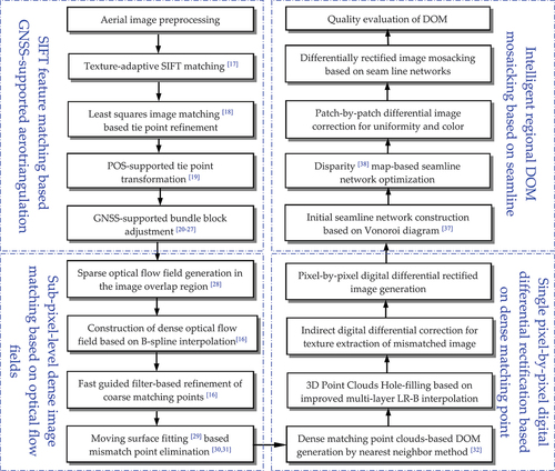
From Figure 1, it is easy to see that most of the individual techniques involved in the method proposed in this paper are relatively mature and need not be described here. However, the automatic hole-filling in densely matched point clouds and the automatic extraction of the DOM seamline network are the two major constraints.

2.1. Automatic hole-filling of 3D point clouds

The 3D point clouds generated by optical flow field-based dense matching of the aerial image pair is textured. As far as the successful matching points are concerned, it is extremely easy to produce a DOM from them, and the grayscale values of the differential rectification image elements can be obtained through nearest-neighbor interpolation. However, for the regions where the failed matching points are clustered, and holes are produced, their grayscale values can only be calculated by the indirect digital differential rectification method. Therefore, the key of the proposed method lies in the automatic detection and completion of the hole during 3D point clouds.

In general, the traditional method of 3D point cloud completion is to use the neighboring points around the hole areas as the reference points and estimate the elevation value of each grid point within the hole by interpolation. Such methods are often ineffective for areas with large holes and complex topographic changes, making the completed 3D point clouds unable to represent the real terrain realistically and obtain accurate feature elevation values. This results in large geometric errors in the mosaicking of the digital differential rectification images generated based on the 3D point clouds. Therefore, to achieve automatic completion of the holes based on dense image matching of the optical flow field in the 3D point clouds this work introduces the LR-B algorithm, which is effective in fitting surfaces and curves in computer graphics and computer-aided design (Dokken, Tom, and P 2013). The algorithm first performs preliminary completion to the 3D point clouds with holes and then refines the patched holes by constructing a globally optimized energy function and a multi-layer B-spline interpolation model with Triangulated Irregular Network (TIN) constraints. Figure 2 illustrates the overall flow of the proposed algorithm.

Figure 2. Flowchart of 3D point cloud completion.

2.1.1. Initial hole-filling surface construction based on locally refined B-spline (LR-B) fItting algorithm

Given a non-decreasing sequence $\mathit{u}=\left(u_0,u_1,u_2,\dots ,\text{break}{u}_n\right)$, a B-spline function with degrees of freedom $\mathrm{n}$ can be represented by the following recursive function (Dokken, Tom, and P 2013):

$B\left[\mathit{u}\right]\left(u\right)=\frac{u-u_0}{u_n-u_0}B\left[u_0,u_1,\dots ,u_n\right]\left(u\right)\text{break}+\frac{u_{n+1}-u}{u_{n+1}-u_1}B\left[u_1,u_2,\dots ,u_{n+1}\right]\left(u\right)$

(1) $B\left[u_i,u_{i+1}\right]=\left\{\begin{array}{c}1;if{u}_i\le u<u_{i+1};\\ 0;otherwise;\end{array}\right.i=0,1,\dots .,n;$(1)

when $u_{n+1}=u_0$ or the denominator of the Equation (1)(1) $B\left[u_i,u_{i+1}\right]=\left\{\begin{array}{c}1;if{u}_i\le u<u_{i+1};\\ 0;otherwise;\end{array}\right.i=0,1,\dots .,n;$(1) is 0, $B\left[\mathit{u}\right]\equiv 0$.

Based on Equation (1)(1) $B\left[u_i,u_{i+1}\right]=\left\{\begin{array}{c}1;if{u}_i\le u<u_{i+1};\\ 0;otherwise;\end{array}\right.i=0,1,\dots .,n;$(1) , the B-spline space of a single variable can be determined by defining the polynomial count $n$ and the node vector $\mathit{u}=\left\{u_0,u_1,\dots ,u_{N+n-1}\right\}$, where the nodes should satisfy $u_{i+1}\ge u_i$ ($i=0,1,\dots .,N+n-1$) and $u_{i+n+1}>u_i$ ($i=0,1,\dots ,N-1$). However, there are often multiple forms to define a B-spline space according to the above model, and usually a locally supported, non-negative, and divisible minimum support B-spline basis function $B_{i,n}\left(u\right)=B\left[u_i,u_{i+1},\dots ,u_{i+n-1}\right]\left(u\right),$ $i=0,1,\dots ,N-1$ is constructed by selecting consecutive $n+2$ nodes in the node vector $\mathit{u}$ to represent this B-spline space.

To construct a three-dimensional B-spline space, two single-variable B-spline bases $B_{i,p_1}\left(u\right)$ and $B_{j,p_2}\left(v\right)$ can be constructed from two non-decreasing sequences $\mathit{u}=\left(u_0,u_1,u_2,\dots ,u_{p1}\right)$ and $\mathit{v}=\left(v_0,v_1,v_2,\dots ,v_{p2}\right),$ where $p_1\ge 0,p_2\ge 0$. The binary tensor product of the two B-spline products can be expressed as follows:

(2) $B_{i,j,p_1,p_2}\left(u,v\right)=B_{i,p_1}\left(u\right)B_{j,p_2}\left(v\right)$(2)

If $F\left(u,v\right)$ denotes a surface in three dimensions, the surface can be defined by Equation (2)(2) $B_{i,j,p_1,p_2}\left(u,v\right)=B_{i,p_1}\left(u\right)B_{j,p_2}\left(v\right)$(2) as follows:

(3) $F\left(u,v\right)=\sum _{i=0}^{N_1-1}\sum _{j=0}^{N_2-1}{c}_{i,j}{B}_{i,j,p_1,p_2}\left(u,v\right)\in \left[u_{p_1},u_{N_1}\right]\times \left[v_{p_2},v_{N_2}\right]$(3)

where $c_{i,j}\in R^d,i=0,\dots ,N_1-1,j=0,\dots ,N_2-1$ is the surface parameter and $d$ is the dimension of the geometric space.

In the case of a two-dimensional B-spline curve, an effective change in the shape of the B-spline curve can be achieved by increasing the number of nodes or by controlling the parameters of the nodes, as shown in Figure 3. Figure 3(a) illustrates the initial B-spline curve and its corresponding nodes. Figure 3(b) reveals that adding nodes inside the initial B-spline curve does not change the shape of the curve, and Figure 3(c) shows the change of the curve after modifying the parameters of the nodes.

Figure 3. Knot insertion of a B-spline curve.

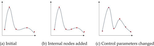
As can be observed from Figure 3, the purpose of controlling the shape of the B-spline curve can be achieved by adding effective control information at specific locations, thus enabling a more accurate representation of changes in feature elevation based on the adjusted interpolation function. In terms of the local refinement B-spline algorithm, as the objective is a 3D surface fitting function, all nodes are projected onto a 2D plane, and the entire control grid can be refined by adding node lines parallel to the grid for each node on the plane. For areas with flat terrain, the control grid can be divided by node lines with larger spacing. Further, the control grid can be refined to enrich the interpolated 3D surface with more detailed information for areas with large terrain undulations and complex features. For the inserted node lines, each must be able to be split into at least one tensor product support region, as shown in Equation (2)(2) $B_{i,j,p_1,p_2}\left(u,v\right)=B_{i,p_1}\left(u\right)B_{j,p_2}\left(v\right)$(2) , and the nodes generated by the inserted grid lines can be used to add new nodes in the uni-variate B-spline function. Refinement must be performed in the direction of the parameters orthogonal to the grid lines in all the B-spline product support regions that are split by the lines. This approach for local refinement can ensure a generated B-spline space more approximate to the real terrain.

An LR-B surface function $F\left(x,y\right)=P_i{B}_i\left(x,y\right)$ ($P_i$ is a parameter of the surface) can be generated for 3D point clouds with holes using the above local B-spline refinement algorithm, and the surface can be refined by the multi-layer B-spline algorithm. Assuming that the times of refinements is k, the final refined surface function can be expressed as follows:

(4) $F\left(x,y\right)=\sum _{i=1}^k{F}_i\left(x,y\right)$(4)

For each B-spline product in the LR-B surface function $B_i$, assuming that the elevation residual at each point on the surface at the kth or k − 1th refinement is $R_t=z_t-F\left(x_t,y_t\right),t\in T$, and $T$ is the support region for $B_i$, a new B-spline residual surface can be constructed based on this residual value, and the surface parameter $qi$ can be calculated from Equation (5)(5) $q_i=\frac{\sum _{i=1}^N{B}_i{\left(x_t,y_t\right)}^2{\varphi }_{i,t}}{\sum _{i=1}^N{B}_i{\left(x_t,y_t\right)}^2}$(5) as follows:

(5) $q_i=\frac{\sum _{i=1}^N{B}_i{\left(x_t,y_t\right)}^2{\varphi }_{i,t}}{\sum _{i=1}^N{B}_i{\left(x_t,y_t\right)}^2}$(5)

where ${\varphi }_{i,t}$ is determined by computing the minimum value of $E=\sum _{i=1}^N{\left(q_i{B}_i\left(x_t,y_t\right)-{\varphi }_{i,t}{B}_i\left(x_t,y_t\right)\right)}^2$. Thus, the LR-B surface function after multi-layer B-spline optimization can be expressed as follows:

(6) $F\left(x,y\right)=F_1\left(x,y\right)+\sum _{i=1}^{k-1}{Q}_i{B}_i\left(x,y\right)$(6)

where $Q_i$ is the set of $q_i$ in the i-th layer of the B-spline residual surfaces.

The LR-B surface function constructed by the local B-spline fitting algorithm and the generated interpolated 3D point cloud will be used as initial values to be input into subsequent optimization algorithms to further improve the effectiveness and accuracy of point cloud hole completion.

2.1.2. Global optimization algorithm for 3D point cloud interpolation under TIN constraints

After multi-layer B-spline refinement, the generated LR-B surface is already refined locally, but these surfaces are often so smooth that the real details at the edges of the terrain features and in regions of abrupt feature elevation changes can be smoothed out, especially in hole regions, making it prone to local over-fitting, which is not globally optimal. Traditional methods for generating DEM and Digital Surface Model (DSM) often adopt the TIN model, which represents better the real feature elevation changes. However, for high-density 3D matched point clouds, the data itself can already represent the 3D topographic relief well, and hence there is no need to construct a TIN as a whole. Consequently, for the completion of 3D point clouds, this paper proposes a least-square global optimization method based on TIN constraints to generate surfaces with estimable terrain details in accordance with the refined 3D surface from the Multi-level B-spline Approximation (MBA) (Lee, Wolberg, and Yong 1997).

For the hole regions with dense matching 3D point clouds, a 3D surface model of the hole regions is first recovered by constructing an irregular triangular network. Based on the 3D model, grid dots are taken out according to the planar grid spacing and incorporated into the original 3D point clouds to generate a complete 3D observation point cloud set $O\left(x,y,z\right)$. Finally, the following global optimized energy function is constructed to minimize the distance between the LR-B surface and the real 3D point clouds.

(7) $\begin{array}{rl}& E={\alpha }_1{E}_{data}+{\alpha }_2{E}_{smooth}\\ & E_{data}=\sum _{i=0}^n{\left(F\left(x_i,y_i\right)-z_i\right)}^{{ }_2},\left(x_{i,}{y}_i,z_i\right)\in O\\ & E_{smooth}=\sum _{i=0}^n\mathcal{L}\left(F\left(x_i,y_i\right),z_i\right),\left(x_i,y_i,z_i\right)\in O\end{array}$(7)

The constants ${\alpha }_1$ and ${\alpha }_2$ are taken as ${\alpha }_1=0.9$ and ${\alpha }_2=0.1$. The data term $E_{data}$ is used to constrain the distance between the fit function and the target observations; the smoothing term $E_{smooth}$ is used to judge whether the elevation trend in the LR-B data is consistent with that of the point cloud observations after the triangulation network constraint in the local hole regions. The algorithm is specified as follows:

(8) $\mathcal{L}=\left\{\begin{array}{c}0,if\left(F\left(x_i,y_i\right)-F\left(x_{i+1},y_{i+1}\right)\right)\times \left(z_i-z_{i+1}\right)>0\\ 1,otherwise\end{array}\right.$(8)

Based on this energy function, the LR-B surface with the smallest energy function value obtained according to the least square criterion is used as the final hole completion surface. Finally, the elevation value on the fitted surface is taken as the elevation of the grid dots on the surface according to the set planar grid size, so as to generate a complementary regular grid dense 3D point clouds.

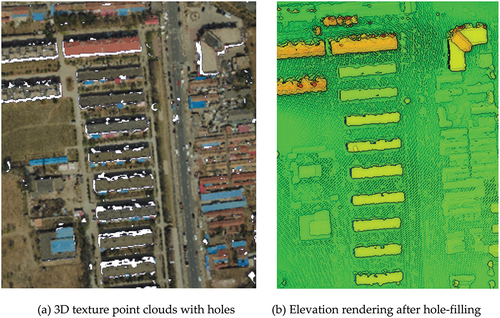
Figure 4 illustrates the completion effect of dense matching point cloud holes in a high-rise building area. From Figure 4(a), it can be clearly observed that there are obvious matching point cloud holes all around the buildings. As shown in Figure 4(b), the edge contour of the buildings is clear and the elevations of the corresponding hole points are basically consistent with the surrounding ground after the multi-layer LR-B interpolation repair with triangular mesh constraint, which means a relatively satisfactory interpolation result.

Figure 4. 3D point clouds completion.

2.2. Automatic extraction of mosaic line networks

The key to the production of a high-quality DOM is to generate a network of mosaic lines that can cover all the digital differential rectification images to be stitched. The network can realize a seamless DOM only if it ensures a reasonable image topology relationship and can completely avoid the different regions between images. In this study, the extraction method of the seamline network is completed in two steps: initial seamline search and seamline optimization in the overlap area.

2.2.1. Automatic generation of the initial mosaic line network

First, the effective zone boundary vector of each differential rectification image is extracted. The effective zone boundary vector of two adjacent differential rectification images is intersected, and the intersection point will be used as the initial mosaic line node. The edges of the overlapping areas on both sides of the node are used as seeds to obtain the best segmentation lines as the initial mosaic lines of the two differentially rectified images through a region growing algorithm. Finally, the bounding box-based Voronoi diagram method (Chen, Zhou, Li, et al. 2019) is adopted to gather all the initial mosaic lines to form the initial seamline network.

2.2.2. Fast optimization of the initial mosaic lIne network

The initial seamline network automatically generated above is optimized here by constructing the disparity map of the two images to be stitched (Yuan, Duan, and Cao 2015). The main optimization process is illustrated in Figure 5.

Figure 5. Flowchart of the seamline network optimization.

First of all, all the corresponding initial mosaic lines of a random differential rectification image are used as seeds to expand the differentially rectified images on both sides and to find the overlapping buffer of the two images. In this work, the buffer radius is adaptively set to 0.2 times the maximum width of the effective area of a single differentially rectified image.

Secondly, the Semi-Global Matching (SGM) algorithm is adopted to generate the disparity map of the buffer D (Pang et al. 2016), which replaces the global optimization of the image by dynamic planning in multiple directions of the pixels to be matched. It can not only significantly reduce the computation time but also basically retain the disparity effect of global optimization so that the height information of buildings, trees, and other objects above the ground can be revealed, thus laying the foundation for a better cost map for automatic mosaic line search.

Then, the obtained disparity map B is divided into the obstacle and non-obstacle binary maps using the threshold segmentation method. For regions within the image coverage area where the topographic relief is relatively flat, the global threshold can be used for direct segmentation. However, in scenes such as cities, the results are not completely satisfied when using a single threshold segmentation owing to the presence of abruptly changing areas at houses, trees, etc. In this study, an adaptive moving threshold segmentation method (Chen et al. 2018) is used to obtain higher quality segmentation results. The segmentation value for each pixel can be calculated as follows:

(9) $B(r,c)=\left\{\begin{array}{c}255,\mathrm{i}\mathrm{f}D(r,c)>T(r,c)\\ 0,\mathrm{o}\mathrm{t}\mathrm{h}\mathrm{e}\mathrm{r}\mathrm{w}\mathrm{i}\mathrm{s}\mathrm{e}\end{array}\right.$(9)

In Equation (9)(9) $B(r,c)=\left\{\begin{array}{c}255,\mathrm{i}\mathrm{f}D(r,c)>T(r,c)\\ 0,\mathrm{o}\mathrm{t}\mathrm{h}\mathrm{e}\mathrm{r}\mathrm{w}\mathrm{i}\mathrm{s}\mathrm{e}\end{array}\right.$(9) , B(r, c) is the gray value of the pixel of the segmented binary map (r, c); D(r, c) is the grayscale of the pixel of the disparity map (r, c); and the threshold T(r, c) is the average grayscale of the N × N neighboring pixels of the disparity map (r, c). When N is set to a small value, the image details can be well preserved, but holes are created in the obstacle region, but when N is set to a larger value, particularly obvious obstacles can be accurately detected, while the image details may be lost. For this reason, a smaller value of N is chosen in this study to ensure that obvious non-ground objects can be segmented effectively.

Finally, the cost image M of the segmented binary image B is generated to obtain the optimal mosaic line by finding a path with the minimum cumulative cost using the improved Dijkstra’s algorithm (Huang 2017). The algorithm is specified as follows.

The edges are extracted from the binary image B obtained from the segmentation, the points of which are then used to construct the Delaunay Triangular Network (DTN). The whole DTN is considered as an undirected graph G(E,V) (here V is the vertex of the graph, and E is the edge of the graph). This transforms the mosaic line search into a path search for a cumulative minimum cost on the undirected graph G(E,V).

The cost value for each pixel of the cost image M can be calculated as follows:

(10) $cos\mathrm{t}(r,c)=\left\{\begin{array}{c}g(r,c)+h(r,c)+1000,\mathrm{i}\mathrm{f}B(r,c)>0\\ g(r,c)+h(r,c),\mathrm{o}\mathrm{t}\mathrm{h}\mathrm{e}\mathrm{r}\mathrm{w}\mathrm{i}\mathrm{s}\mathrm{e}\end{array}\right.$(10)

In Equation (10)(10) $cos\mathrm{t}(r,c)=\left\{\begin{array}{c}g(r,c)+h(r,c)+1000,\mathrm{i}\mathrm{f}B(r,c)>0\\ g(r,c)+h(r,c),\mathrm{o}\mathrm{t}\mathrm{h}\mathrm{e}\mathrm{r}\mathrm{w}\mathrm{i}\mathrm{s}\mathrm{e}\end{array}\right.$(10) , cost(r, c) is the cost value of the cost image pixel (r, c); g(r,c) is the cumulative path distance of the pixel from the starting point of the mosaic; and h(r,c) is the distance of the pixel to the end of the search. When the value of the pixel on image B equals 0, i.e. when it falls into the traversable region, its cost value is g(r,c) + h(r,c); when the value of the pixel on image B is greater than 0, the cost value of the pixel is g(r,c) + h(r,c) + 1000, which means that the pixel falls into the impassable region, while the cost value increased by 1000 penalties.

For the vertex V_i in an undirected graph G(E,V), the cost value cost_Vi of this vertex can be computed by finding the corresponding pixel on the cost image M, and the weight of the edge E_ij formed by the vertices V_i, V_j is set to be weight(E_ij) = cost_Vi + cost_Vj.

Once the weights of all edges in the undirected graph G(E,V) are computed, the optimal mosaic line search consists of obtaining the weights on the path and the minimum path.

(11) $min\sum _{V_i,V_j\in path}\mathrm{w}\mathrm{e}\mathrm{i}\mathrm{g}\mathrm{h}\mathrm{t}(E_{ij})$(11)

Compared with traditional pixel-by-pixel path search algorithms, the improved Dijkstra algorithm proposed here can significantly increase the search efficiency.

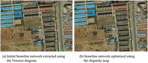
Figure 6 illustrates a network of fully automated extracted mosaic lines in a dense area of high-rise buildings, where the green lines are mosaic lines and the numbers are image names. It can be clearly observed from the figure that the optimized mosaic lines are all well ahead along the areas with small projection differences, which can minimize the geometric jointing error of the features during DOM mosaicking.

Figure 6. Fully automatic extraction of the seamline network in a dense area of buildings.

2.3. Experimental design

To verify the effectiveness and applicability of the proposed method and to evaluate comprehensively the quality of the automatically produced DOM. Three sets of aerial images taken from different areas were selected for the experiment. The first set of images is the low-altitude aerial photography of a suburban area in Beijing (capital of China), covering mainly blocks of cultivated land, urban roads, street gardens, dense low-rise residential areas, and planned high-rise residential buildings; the second set is the conventional aerial photography of the seaside of Preserver Island in Shandong Province, China, which mainly comprises marine farms and facilities, dams, woods, farmlands, factories, and villages. The third set of images is provided by ISPRS benchmark, covering a urban city area of Vahingen, Germany. The parameters of the three sets of aerial images are listed in Table 1.

Table 1. Parameters for the two sets of experimental images.

Item	Beijing	Preserver Island	Vahingen
Aerial craft	Low-altitude Unmanned Aerial Vehicles (UAV)	Chinese transport 12 aircraft	Aircraft
Camera	Phase One IXU-1000	Phase One RS-1900	Intergraph/ZI DMC
Date of aerial photography	May 2016	November 2017	August 2008
Principal distance (mm)	51.212,93	89.470,90	120.000,00
Format (pixels)	11,608 × 8708	11,540 × 16,470	7680 × 13,824
Pixel size (µm)	4.6	4.6	12.0
Ground Sample Distance (GSD) (cm)	7	5	8
Relative flight height (m)	779	960	900
Longitudinal overlap (%)	60	60	60
Lateral overlap (%)	30	40	60
Number of mapping strips	4	8	3
Number of control strips	4	2	1
Number of Images	88	268	20
Number of Ground Control Points (GCPs)	20	25	0
Number of pass points	161,085	113,670	7151
Block area (km^2)	2.8 × 2.8	5.2 × 5.2	2.1 × 1.8
Maximum topographic relief (m)	60	20	170
Average ground elevation (m)	507	49	285
Image matching accuracy (μm/pixels)	±0.8 / ±0.17	±1.0 / ±0.22	±2.88 / ±0.24
Pass point planimetric/height accuracy (m)	±0.070 / ±0.065	±0.066 / ±0.073	±0.089 / ±0.103

Our self-developed fully automatic digital photogrammetry system, named Imagination, was used as the data processing platform. First, the automatic image measurement subsystem (Imagination-AMS) of the platform was used for the automatic tie point measurement of the two sets of images. Artificial stereometry of the image points of all the GCPs was then performed. Subsequently, the camera station positioning subsystem referred to as (Imagination-GNSS) because it utilizes a Global Navigation Satellite System (GNSS) camera, was used to obtain the 3D coordinates of all the camera stations based on the GPS precision single point positioning via carrier phase observations recorded during the aerial photographing. Next, the 3D ground coordinates of the pass points were adjusted by GPS-supported bundle block adjustment subsystem (Imagination-BBA). In order to improve the height accuracy of the pass points, a generally recommended ground control scheme to use four of the GCPs at the four corners of the block and two control strips on the start and end of the block was adopted. The unit weight RMSE of the image point coordinate observations was less than ±0.25 pixels, and the planimetric and height accuracy of the photogrammetric determination reached the cm level in the ground, approaching the level of ±1.0 GSD (see the last two rows in Table 1 for details). Then, the DSM automatic extraction subsystem (Imagination-DEM) was further used to implement dense image matching based on the OFFDIM, and using the classical dual-image spatial intersection method in photogrammetry, the 3D point clouds were automatically generated. Finally, the DOM automatic generation subsystem (Imagination-DOM) was further used to produce DOM according to the proposed method in this paper. The first and second datasets are utilized for a comprehensive study of the proposed method, the comparison experiment is conducted on the smaller sized open sourced benchmark dataset provided by ISPRS society due to the processing limitation of the commercial softwares (SURE and Agisoft PhotoScan). The detailed experimental results and discussions are presented in Section 3.

3. Experimental results and discussions

3.1. DOM with typical features

The uniformly distributed image tie points obtained by photogrammetry determination were used as seed points, and dense matching based on the optical flow field was performed on all mapping strip images of the two experimental blocks. After automatic extraction of 3D point clouds and hole area completion, the DOM image element size was set to the GSD of the aerial images, and the DOM of the entire area was generated automatically through the process in Figure 1. Because the length of this paper is limited, Figure 7 only shows the local DOM of 10 typical objects.

Figure 7. Doms of ten typical surface features generated by the fully automatic method proposed in this paper.

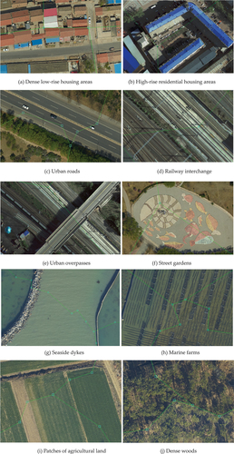
In terms of the visual effects of the DOMs of the two experimental areas, the image texture is clear and layered, without any blurring, misalignment, distortion, or pulling of features. The entire DOMs have saturated color, moderate contrast, and uniform tones, with no obvious noise or geometric distortion. After superimposing the mosaic lines on the locally enlarged DOM images of the 10 typical objects in Figure 7, it can be clearly observed that each DOM is mosaicked from three to four differential rectification images. From a geometric point of view, there is no obvious projection difference between the differential rectification images, and there is no substantial geometric mosaic error; from a radiometric point of view, the color transition between the differential rectification images is natural, and there is no obvious radiometric difference. This subjectively determines that the DOM produced by the method in this paper is of high quality.

3.2. Evaluation of DOM accuracy

To evaluate the quality of the DOM objectively, this study applied a statistical method to quantify the DOM accuracy using two main indicators: the RMSE on the jointing edge of the differential rectification images and the RMSE in the planimetric position of the DOM check points.

1) Jointing edge accuracy of differential rectification images: all seamline segments of two adjacent differential rectification images were sequentially extracted to form a statistical seamline unit based on the optimized seamline network. Taking the statistical seamline as the center line and 100 pixels as the bandwidth, a buffer was constructed in each of the two differential rectification images to be mosaicked, and feature matching of the Harris corner points was performed on the buffer image (Harris and Stephens 1988). Due to the varying lengths of the statistical seamlines and the different textures of the images they cross, the matching yielded a range of 20 to 300 points of the same name. From the deviations in the positions of these matching points, the RMSE in the jointing edge of the statistical seamline was calculated as follows:

(12) ${\mu }_M=\sqrt{\frac{1}{n}\sum _{i=1}^n[(X_L-X_R{)}_i^2+(Y_L-Y_R{)}_i^2]}$(12)

Where, n is the number of matching points, and (X_L , Y_L) and (X_R, Y_R) are the ground coordinates of the same name points on the two differential rectification images, respectively.

Similarly, the RMSE in the jointing edge of each statistical seamline in the seamline network was calculated in turn, and the mean value${\bar{\mu }}_M$ was used as a measure of the jointing edge accuracy of the differential rectification images.

2）Planimetric position accuracy of DOM: Using ground control points measured in the field as checkpoints, the DOM surface coordinates of the checkpoints were read one by one with Imagination’s DOM measurement tools to obtain the planimetric position errors by differentiating with the ground measurement coordinates. Finally, the planimetric position errors were counted as the accuracy measurement of the DOM.

(13) ${\bar{\mu }}_{DOM}=\sqrt{\frac{1}{n}\sum _{i=1}^n[(X_C-X_M{)}_i^2+(Y_C-Y_M{)}_i^2]}$(13)

where n is the number of checkpoints; (X_C, Y_C) and (X_M, Y_M) are the measured and plot coordinates of the checkpoints, respectively.

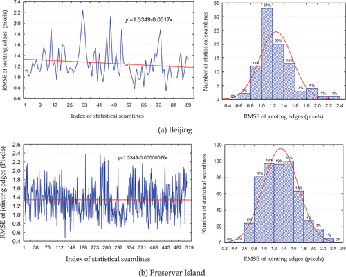
Figure 8 plots the accuracy trends and statistical histograms for the jointing edges of all differential rectification images in the two experimental areas.

Figure 8. Mosaic accuracy curves and histograms between differential rectification images.

From the analysis of Figure 8, the following aspects can be observed:

1. In terms of the RMSE of the differential rectification images, there is some difference in the individual images due to different feature coverage and overlapping, but the difference is only within 1.5 pixels. The reason is that the images within the mapping strips are highly overlapped in heading, and they are intensively matched, achieving the best accuracy of ±0.45 pixels; the images between the strips are slightly less accurate than those within the strips because they are not intensively matched in the overlap area for their small overlap in the side direction.

2. The overall jointing edge accuracy fitting curves of the differential rectification images in both experimental areas are straight lines. In Beijing, the experimental area with a smaller sample size, there are 40 differential rectification images and 89 statistical seamlines. The maximum accuracy difference is 1.1 pixels. The slope of the fitted straight line of −0.0017 pixels/line, which is approximately horizontal. In Preserver Island, the experimental area with a larger sample size, there are 233 differential rectification images and 511 statistical seamlines, which is almost a horizontal line. However, the intercepts of both fitted lines are equal to 1.3349 pixels, which indicates that the overall accuracy of the rectified images in the two experimental areas is consistent.

3. The jointing edge accuracy of a single statistical seamline is better than ±2.4 pixels, and that of approximately 80% of the statistical seamlines is better than ±1.5 pixels. Table 2 also shows that the overall jointing edge accuracy is better than ±1.5 pixels. This fully demonstrates that the pixel-by-pixel digital differential rectification accuracy using the method proposed in this paper is fairly high. Although affected by factors such as features and image resolutions, the rectification error is generally uniformly distributed, which is strongly beneficial to DOM mosaicking. It not only ensures the geometric accuracy of the DOM but also reduces the complexity of DOM mosaicking, thus improving its automation. This objectively corroborates the subjective good visual effect shown in Figure 4.

Table 2. DOM accuracy for the two experimental areas.

Experimental area	DOM cell size (m)	Seam accuracy			DOM accuracy
		Number of seam lines	Maximum edge error (m/pixels)	${\bar{\mu }}_M$ (m/pixels)	Check points	Maximum point error (m/pixels)	${\bar{\mu }}_{DOM}$ (m/pixels)
Beijing	0.070	89	0.157 / 2.24	0.090 / 1.28	15	0.175 / 2.50	0.078 / 1.11
Preserver Island	0.050	511	0.119 / 2.38	0.069 / 1.39	25	0.116 / 2.32	0.057 / 1.14

Table 2 presents the accuracy statistics of the DOM produced fully automatically for the two experimental areas according to Equations (1)(1) $B\left[u_i,u_{i+1}\right]=\left\{\begin{array}{c}1;if{u}_i\le u<u_{i+1};\\ 0;otherwise;\end{array}\right.i=0,1,\dots .,n;$(1) and (2(2) $B_{i,j,p_1,p_2}\left(u,v\right)=B_{i,p_1}\left(u\right)B_{j,p_2}\left(v\right)$(2) ).

According to the provisions of China’s mapping industry standard, “Digital Results of Basic Geographic Information 1:500, 1:1000, 1:2000 Digital Orthophoto Maps,” the RMSE of the planimetric position of the flat 1:500 scale DOM should be less than ±0.3 m (2011). Compared with the results presented in Table 2, it is not difficult to find that the geometric accuracy of the DOM produced fully automatically using the method proposed in this paper entirely meets the current specification requirements, and the DOM accuracy is better than twice the specification tolerance, close to the level of 1.0 GSD. Even the maximum point error does not exceed 2.5 GSD, less than 2/3 of the limit difference. This further demonstrates that the DOM produced by the method proposed in this paper is very accurate.

3.3. Comparison with state-of-the-art methods

The comparison experiment is conducted with a high-end DELL workstation with Intel i9 11900KF CPU, 64GB RAM, and Nvida GTX3090ti GPU. For Agisoft PhotoScan, ISPRS society provides interior and exterior camera parameters that are used to establish the mapping project and process the DOM generation automatically with the default settings. For SURE, the Photoscan established project file is utilized as the initial input, and follows its dense stereo matching, DEM generation, ortho-rectification, and mosaicking pipeline to automatically generate the DOM. The visual comparison of the proposed method with SURE and Agisoft PhotoScan is shown in Figure 9.

Figure 9. Visual comparison of the automatically generated DOMs on the Vahingen dataset.

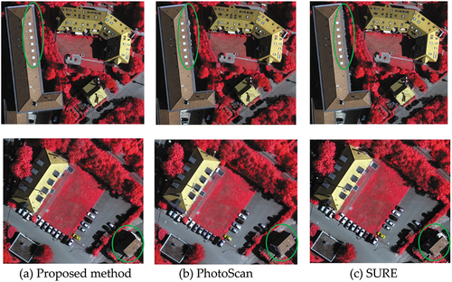
According to Figure 9, the proposed method generated DOM shows the most smoothness and completeness on building edges. PhotoScan generated DOM may show some larger distortions on the tall building edges, and for some small parts, the building facades are not rectified. The SURE generated DOM also shows some sawtooth noise around the tall building boundaries. And for some gable roofs it may show some distortion and incompleteness which may cause by the mismatching and incompleteness of the dense point clouds.

The accuracy comparison of the three methods is shown in Table 3. Comparing the generated DOM accuracy, three methods are at the same level, SURE is slightly higher than the proposed method while PhotoScan is slightly lower than the proposed method, this is because PhotoScan utilizes the ground filtering method to exclude the ground objects when generating the DEM, which may cause some distortions when otho-rectification. Comparing to the state-of-the-art commercial softwares, the proposed methods spent fewer time to do the otho-rectification, meanwhile, we only utilize CPU as the computational resources, other two softwares utilize GPU to accelerate the computation, which demonstrated that the proposed method is computational efficiency than the other two methods.

Table 3. Quantitative comparison of the three methods.

Method	DOM cell size (m)	Processing time			DOM accuracy
		Dense image matching (min)	DEM generation (min)	Ortho rectification (min)	Check points	Maximum point error (m/pixels)	${\bar{\mu }}_{DOM}$ (m/pixels)
Proposed	0.080	27.4	5.3	5.2	10	0.208 / 2.51	0.121 / 1.51
PhotoScan	0.080	25.1	12.1	7.4	10	0.210 / 2.62	0.139 / 1.74
SURE	0.080	31.2	4.5	6.2	10	0.190 / 2.37	0.115 / 1.44

From Table 3, through the comparison experiment with the state-of-the-art commercial software, the proposed method generated DOM achieved a ± 1GSD level accuracy, with less distortion in building boundary area and fewer noises. And the overall processing time improved by nearly 15%.

4. Conclusions

This paper describes the basic principles and detailed process of pixel-by-pixel digital differential rectification using dense matching point clouds of aerial images. From the experiments and quality analysis of DOM production in the two experimental areas, the following conclusions and recommendations can be made.

1. The method proposed in this paper can truly realize pixel-by-pixel digital differential rectification. For aerial images, it is a mode of operation that generates DOM directly from densely matched point clouds without any dependence on the DEM and/or time-consuming and laborious DEM editing operations. It will revolutionize the current DOM production model in terms of the production process.

2. The accuracy of DOMs produced using the method presented in this paper is close to the level of GSD in the field. The geometric accuracy of the produced DOMs is much higher than the accuracy requirements for large-scale DOMs of China’s basic geographic information digital results, showing no obvious geometric misalignment of the feature edges and natural color transition. This reveals that this method has great accuracy potential and broad application prospects in practical production.

3. The proposed method is a DOM production method that strictly follows the photogrammetry principles. In accordance with the DOM production process flow of aerial triangulation, pixel-by-pixel 3D point cloud extraction, pixel-by-pixel digital differential rectification, and orthographic projection image mosaicking, every step here can be performed automatically with almost no human intervention. Thus, this method can achieve the long-awaited goal of fully automated DOM production in one click.

Owing to the limitation of experimental data, the experiments carried out in this study were mainly for flat lands, and they need to be expanded to mountainous areas and urban areas with high-rise buildings. There is still room for further improvement in the completion of point cloud holes and automatic extraction of mosaic line networks, especially regarding the efficiency of the algorithm.

Disclosure statement

No potential conflict of interest was reported by the authors.

Data availability statement

Some data that support the results and analyses presented in this paper are freely available online (URLs: https://pan.baidu.com/s/1mQCQNjW9eGaesfxsYQqcaw Password: hsly). Others cannot be shared at this time, as the data also form part of an ongoing study.

Additional information

Funding

This work is supported by the National Natural Science Foundation of China [Grant No. 41771479], the National High-Resolution Earth Observation System (the Civil Part) [Grant No. 50-H31D01-0508-13/15] and the Japan Society for the Promotion of Science [Grant No. 22H03573].

Notes on contributors

Wei Yuan

Wei Yuan received the PhD degree from Wuhan University and The University of Tokyo. His research interests are photogrammetry and remote sensing, dense image matching, object detection, and change detection.

Xiuxiao Yuan

Xiuxiao Yuan received his PhD degree from Wuhan University His research interests are aerial triangulation, bundle block adjustment, and error processing.

Yang Cai

Yang Cai is a PhD students at Wuhan University. His research interests are ortho-image rectification, and automatic seamline detection.

Ryosuke Shibasaki

Ryosuke Shibasaki is a professor at the University of Tokyo, his research interests are remote sensing image processing, geospatial information science, and human mobility prediction.

References

- Ackermann, F. 1979. “The Concept of Reliability in Aerial Triangulation, Ricerche di Geodesia Topografiae Fotogrammetria.” Cooperativa Libraria Universitaria del Polytecnico.
- Ackermann, F. 1984. “Digital image correlation: performance and potential application in photogrammetry.” The Photogrammetric Record 11 (64): 429–439.
- Ackermann, F. 1992. “Prospects of Kinematic GPS for Aerial Triangulation.” ITC Journal 4: 326–328.
- Ackermann, F. 1994. “Practical Experience with GPS Supported Aerial Triangulation.” Photogrammetric Record 14 (84): 860–874. doi:10.1111/j.1477-9730.1994.tb00287.x.
- Baltsavias, E. P. 1996. “Digital Ortho-Images—A Powerful Tool for the Extraction of Spatial-And Geo-Information.” Isprs Journal of Photogrammetry and Remote Sensing 51 (2): 63–77. doi:10.1016/0924-2716(95)00014-3.
- Chen, G., S. Chen, X. Li, P. Zhou, and Z. Zhou. 2018. “Optimal Seamline Detection for Orthoimage Mosaicking Based on DSM and Improved JPS Algorithm.” Remote Sensing 10 (6): 821. doi:10.3390/rs10060821.
- Cheng, G., X. Xie, W. Chen, X. Feng, X. Yao, and J. Han. 2022. “Self-Guided Proposal Generation for Weakly Supervised Object Detection.” IEEE Transactions on Geoscience and Remote Sensing 60: 1–11. doi:10.1109/TGRS.2022.3181466.
- CH/T 9008.3-2010. 2011. Digital Products of Fundamental Geographic Information 1:500 1:1000 1:2000 Digital Orthophoto Maps. Beijing: Surveying and Mapping Press.
- Deren, L., and S. Jie. 1989. “Quality Analysis of Bundle Block Adjustment with Navigation Data.” Photogrammetric Engineering and Remote Sensing 55 (12): 1743–1746.
- Dokken, T., L. Tom, and K. F. P. 2013. “Polynomial Splines Over Locally Refined Box-Partitions.” Computer Aided Geometric Design 30 (3): 331–356. doi:10.1016/j.cagd.2012.12.005.
- Erickson, B. D., and K. Biedenweg. 2022. “Distrust Within Protected Area and Natural Resource Management: A Systematic Review Protocol.” Plos One 17 (3): e0265353. doi:10.1371/journal.pone.0265353.
- Gao, Z., Y. Song, C. Li, F. Zeng, and F. Wang. 2017. “Research on the Application of Rapid Surveying and Mapping for Large Scale Topographic Map by Uav Aerial Photography System.” The International Archives of Photogrammetry, Remote Sensing and Spatial Information Sciences 42: 121. doi:10.5194/isprs-archives-XLII-2-W6-121-2017.
- Harris, C., M. Stephens. 1988. “A Combined Corner and Edge Detector.” The 4th Alvey Vision Conference, Manchester, England, 147–151.
- Huang, Y. 2017. “Research on the Improvement of Dijkstra Algorithm in the Shortest Path Calculation.” The 4th International Conference on Machinery, Materials and Computer, Xian, China, Atlantis Press.
- Lee, K., J. H. Kim, H. Lee, J. Park, J. P. Choi, and J. Hwang. 2021. “Boundary-Oriented Binary Building Segmentation Model with Two Scheme Learning for Aerial Images.” IEEE Transactions on Geoscience and Remote Sensing 60: 1–17. doi:10.1109/TGRS.2021.3089623.
- Lee, S., G. Wolberg, and S. Yong. 1997. “Scattered Data Interpolation with Multilevel B-Splines.” IEEE Transactions on Visualization and Computer Graphics 3 (3): 228–244. doi:10.1109/2945.620490.
- Li, Q., L. Mou, Y. Hua, Y. Shi, and X. Zhu. 2021. “Building Footprint Generation Through Convolutional Neural Networks with Attraction Field Representation.” IEEE Transactions on Geoscience and Remote Sensing 60: 1–17. doi:10.1109/TGRS.2021.3109844.
- Liu, Y., X. Zheng, G. Ai, Y. Zhang, and Y. Zuo. 2018. “Generating a High-Precision True Digital Orthophoto Map Based on UAV Images.” ISPRS International Journal of Geo-Information 7 (9): 333. doi:10.3390/ijgi7090333.
- Li, D., and X. Yuan. 2012. Error Processing and Reliability Theory (Second Edit). Wuhan: Wuhan University Press.
- Lowe, D. G. 2004. “Distinctive Image Features from Scale-Invariant Keypoints.” International Journal of Computer Vision 60 (2): 91–110. doi:10.1023/B:VISI.0000029664.99615.94.
- Matikainen, L., M. Lehtomäki, E. Ahokas, J. Hyyppä, M. Karjalainen, A. Jaakkola, A. Kukko, and T. Heinonen. 2016. “Remote Sensing Methods for Power Line Corridor Surveys.” Isprs Journal of Photogrammetry and Remote Sensing 119: 10–31. doi:10.1016/j.isprsjprs.2016.04.011.
- Pang, S., M. Sun, X. Hu, and Z. Zhang. 2016. “SGM-Based Seamline Determination for Urban Orthophoto Mosaicking.” Isprs Journal of Photogrammetry and Remote Sensing 112 (2): 1–12. doi:10.1016/j.isprsjprs.2015.11.007.
- Shi, J., X. Yuan, Y. Cai, and G. Wang. 2017. “GPS Real-Time Precise Point Positioning for Aerial Triangulation.” GPS Solutions 21 (2): 405–414. doi:10.1007/s10291-016-0532-2.
- Song, CH., ZH., Ping, LI., Xianju, CH., Gang 2019. ”Seamline Network Generation and Optimization for Orthoimage Mosaicking Based on Voronoi Diagrams.” Bulletin of Surveying and Mapping 2019 (6): 57–60
- Wang, Z. 1990. Principle of Photogrammetry (With Remote Sensing). Beijing: Publication House of Surveying and Mapping.
- Wang, Y. 2019. “Brief Analysis of Production Method of Orthophoto Image Based on INPHO.” Modern Information Technology 3 (8): 1–3.
- Xie, F., X. Song, and K. Wang. 2013. “A Practical DOM Production Process and Method.” Modern Surveying and Mapping 36 (4): 31–32+35.
- Xiuxiao, Y. 2000. “Principle, Software and Experiment of GPS-Supported Aerotriangulation.” Geo-Spatial Information Science 3 (1): 24–33. doi:10.1007/BF02826803.
- Yang, G., C. Li, Y. Wang, H. Yuan, H. Feng, B. Xu, and X. Yang. 2017. “The DOM Generation and Precise Radiometric Calibration of a UAV-Mounted Miniature Snapshot Hyperspectral Imager.” Remote Sensing 9 (7): 642. doi:10.3390/rs9070642.
- Yang, K., G. Xia, Z. Liu, B. Du, W. Yang, M. Pelillo, and L. Zhang. 2021. “Asymmetric Siamese Networks for Semantic Change Detection in Aerial Images.” IEEE Transactions on Geoscience and Remote Sensing 60: 1–18. doi:10.1109/TGRS.2021.3113912.
- Yuan, X. 2009. “Quality Assessment of GPS-Supported Bundle Block Adjustment Based on Aerial Digital Frame Imagery.” Photogrammetric Record 24 (126): 139–156. doi:10.1111/j.1477-9730.2009.00527.x.
- Yuan, W. 2020. Dense Image Matching and Its Application Based on Optical Flow Field. Wuhan, China: Wuhan University.
- Yuan, X., Y. Cai, J. Shi, and C. Zhong. 2017. “BeiDou-Supported Aerotriangulation for UAV Aerial Images.” Geomatics and Information Science of Wuhan University 42 (11): 1573–1579.
- Yuan, X., M. Duan, and J. Cao. 2015. “A Seam Line Detection Algorithm for Orthophoto Mosaicking Based on Disparity Images.” Acta Geodactica et Cartographica Sinica 44 (8): 877–883.
- Yuan, X., J. Fu, H. Sun, and C. Toth. 2009. “The Application of GPS Precise Point Positioning Technology in Aerial Triangulation.” Isprs Journal of Photogrammetry and Remote Sensing 64 (6): 541–550. doi:10.1016/j.isprsjprs.2009.03.006.
- Yuan, X., and Y. Ming. 2009. “A Novel Method for Multi-Image Matching Synthesizing Image and Object-Space Information.” Geo-Spatial Information Science 12 (3): 157–164. doi:10.1007/s11806-009-0063-x.
- Yuan, W., X. Yuan, S. Xu, J. Gong, R. Shibasaki. 2019. “Dense Image Matching via Optical Flow Field Estimation and Fast Guided Filter Refinement.” Remote Sensing 11 (20): 2410. doi:10.3390/rs11202410.
- Zhang, J., H. Gu, W. Hou, and C. Cheng. 2021. “Technical Progress of China’s National Remote Sensing Mapping: From Mapping Western China to National Dynamic Mapping.” Geo-Spatial Information Science 24 (1): 121–133. doi:10.1080/10095020.2021.1887713.
- Zhang, J., L. Pan, and S. Wang. 2018. Photogrammetry. 2rd ed. Wuhan: Wuhan University Press.
- Zhu, Q., J. Zhang, Y. Ding, M. Liu, Y. Li, B. Feng, S. Miao, W. Yang, H. He, and J. Zhu. 2019. “Semantics-Constrained Advantageous Information Selection of Multimodal Spatiotemporal Data for Landslide Disaster Assessment.” ISPRS International Journal of Geo-Information 8 (2): 68. doi:10.3390/ijgi8020068.