Estimation of global karst carbon sink from 1950s to 2050s using response surface methodology

ABSTRACT

For the estimation of global karst carbon sink, a few conventional methods usually require the parameters that are difficult to measure, resulting in the big cost. Moreover, under the constraints of incomplete and timeliness issues in the collection of data over a large region, it has remained a challenge for these methods to study global karst carbon sink. Therefore, this paper proposes estimating the global karst carbon sink, and analyzing the suitability of the response surface methodology and the fluctuating variation of karst carbon sink in global karst regions from 1951 to 2050. This paper shows that the proposed method can reduce the time of numerical calculation and is suitable for application in global weathering models; The global karst carbon sink in the future changes not only displays an upward trend but also exposures its fluctuating trend largely. This fluctuation is probably due to global warming.

KEYWORDS:

• Earth system
• carbon sink
• response surface methodology
• residual terrestrial carbon sink
• global carbon cycle

1. Introduction

The Earth’s surface undergoes a complex series of interactions between the atmosphere, lithosphere, oceans, and biosphere through energy and material exchange (Moquet et al. 2011). This interaction has been resulting in Earth system dynamics that are changing rapidly and many adjustments are occurring at the Earth’s surface (Nistor 2019). There is still a called “missing carbon sink” happening in the global carbon cycle through ocean, atmospheric, and terrestrial carbon flux balances in global carbon cycle model (Houghton, Davidson, and Woodwell 1998). It has been estimated that the mass of the “missing carbon sink” is 1–2.5 $PgC\cdot {\mathrm{a}}^{-1}$ (Schimel et al. 1996; Gombert 2002; Lal 2007; Liu and Dreybrodt 2015; Liu et al. 2018).

Internationally, the “missing carbon sink” is generally considered to be stored in terrestrial vegetation or soil (Detwiler and Hall 1988; Sarmiento and Sundquist 1992; Fisher et al. 1995; Fan et al. 1998; Lal 2004), or where silicate weathering precipitates and buries atmospheric carbon as solid carbonate minerals (Berner, Lasaga, and Garrels 1983; Zeng, Jiang, and Liu 2016; Liu et al. 2018). However, the influence of carbonate weathering on atmospheric carbon is often ignored (Martin 2017). In accordance with the research results from Gombert (2002), Liu, Dreybrodt, and Liu (2011, 2018) and Gaillardet et al. (2019), the carbon sink formed by carbonate chemical weathering is one of the missing carbon sink. It converts $C{O}_2$ in the atmosphere/soil into $HC{O}_3^{-}$ and releases it into water, creating a carbon sink effect (Liu, Dreybrodt, and Liu 2011; Cao et al. 2016; Liu et al. 2018). Although the processes such as silicate minerals weathering and volcanic recreation have dominated the global carbon cycle on longer time durations (over millennia) (Berner, Lasaga, and Garrels 1983; Berner 2004), the carbon sink fashioned through silicate weathering is restrained due to its sluggish weathering dynamics on quick time durations (Berner 2004; Zeng, Jiang, and Liu 2016; Liu, Dreybrodt, and Liu 2011; Liu et al. 2018). In contrast, carbonate has a faster weathering kinetics than silicate has (White and Brantley 2003; Beaulieu et al. 2012). The Dissolved Inorganic Carbon (DIC) in almost all watersheds (voids, caves, rivers, and lakes) is dominated by carbonate rock (Liu, Dreybrodt, and Wang 2010; Liu, Dreybrodt, and Liu 2011; Liu and Dreybrodt 2015). Meanwhile, the DIC in the watershed photosynthesize with aquatic organisms to produce organic carbon, which is buried in sediments (Liu, Dreybrodt, and Wang 2010; Liu, Dreybrodt, and Liu 2011; Liu and Dreybrodt 2015; Liu et al. 2018; Chen et al. 2017). This conversion from inorganic carbon (carbonate weathering) to organic carbon (aquatic photosynthesis) further enhances the carbon sink effect (Ma et al. 2014). Liu et al. (2018) defined the relationship between carbonate weathering and aquatic photosynthesis as Coupled Carbonate Weathering (CCW). It not only integrates karst carbon sink and organic carbon sink in the catchment but also reduces the calcite saturation in the water, resulting in less calcite precipitation in the sediment and increasing inorganic carbon stability (Adamczyk et al. 2009; Liu, Dreybrodt, and Liu 2011; Zhou et al. 2015; Liu and Dreybrodt 2015; Cao et al. 2016). Therefore, carbonate weathering is a potential carbon sink for atmospheric $C{O}_2$ (Liu and Zhao 2000; Liu et al. 2018), and its contribution to terrestrial carbon sink desires the consideration in a global carbon cycle model, which can present a lookup foundation for analyzing problems such as carbon source-sink imbalances in global carbon cycle model.

After decades of research, it has become accepted that karst carbon sink formed by carbonate weathering are an important component of the global terrestrial missing carbon sink (Liu and Zhao 2000; Liu et al. 2018; Zhou et al. 2020). In the previous research on carbonate weathering, researchers have usually investigated carbonate chemical weathering by employing dynamic method, hydrogeochemistry method and hydrological modeling methods (Amiotte-Suchet and Probst 1995; Dupré et al. 2003; Goddéris et al. 2006; Roelandt et al. 2010; Goddéris et al. 2013; Hartmann et al. 2014; Zhou et al. 2015; Romero-Mujalli, Hartmann, and Börker 2019). The methods can be divided into the following categories.

1. Dynamic Method (DM): dynamic method studies carbonate weathering rate from microscopic perspective, which can better describe rate mechanism and reaction principle of karst. The theoretical models of this method include the PWP model (Plummer, Wigley, and Parkhurst 1978) and the DBL model (Dreybrodt and Buhmann 1991).

   • PWP: Plummer et al. found that the water-rock boundary layer forms a water film whose thickness is influenced by temperature, $C{O}_2$ partial pressure, and liquid composition (Plummer, Wigley, and Parkhurst 1978). The model is $R=b_1{k}_1({\mathrm{H}}^{+})+b_2{k}_2({\mathrm{H}}_2\mathrm{C}{\mathrm{O}}_3)+b_3{k}_3$$({\mathrm{H}}_2\mathrm{O})-b_4{k}_4(\mathrm{C}{\mathrm{a}}^{2+})-b_5({\mathrm{H}\mathrm{C}\mathrm{O}}_3^{-})$, and the equations $k_1$, $k_2$and $k_3$ are temperature-dependent constants; and $k_4$ is not only temperature-dependent but also related to the partial pressure of $C{O}_2$, and b is the activity coefficient of the corresponding composition.

   • DBL: Dreybrod et al. proposed a diffusion boundary layer theory model (Dreybrodt and Buhmann 1991). The model is $R=(a/\epsilon )(D_1-D_2)$, where $a$ is the coefficient of molecular diffusion, which is related to temperature and $C{O}_2$ pressure; $\epsilon$ is the diffusion boundary layer thickness, $D_1$ is the calcium ion concentration on the calcite surface in the diffuse boundary layer, and $D_2$ is the calcium ion concentration in uniform solution.

2. Hydrogeochemistry Method (HM): the hydrogeochemistry method calculates the total amount of ions carried in the river by measuring the concentration of solutes (such as ${\mathrm{H}\mathrm{C}\mathrm{O}}_3^{-}$, ${\mathrm{K}}^{+}$, $\mathrm{N}{\mathrm{a}}^{+}$, $\mathrm{C}{\mathrm{a}}^{2+}$, etc.) in spring water or basin runoff. This method mainly includes the $\mathrm{G}\mathrm{E}\mathrm{M}-\mathrm{C}{\mathrm{O}}_2$ model, SiB algorithm and river chemistry method.

   • $\mathrm{G}\mathrm{E}\mathrm{M}-\mathrm{C}{\mathrm{O}}_2$ model: Amiotte and Probst described a linear relationship between atmospheric $C{O}_2$ and runoff depleted by rock weathering (Amiotte and Probst 1995). The equation is $F=a\cdot Q$, where $a$ is a factor for different rock types; $Q$ is the runoff volume, mm/a.

   • SiB: This method is an algorithm for assessing the weathering rate of minerals by applying the molar equilibrium method (Pacheco and Van der Weijden 2002). It estimates the amount of atmospheric $C{O}_2$ consumed during rock weathering based on the relationship between rock dissolution rate and runoff (Pacheco and van der Weijden 1996).

   • River chemistry method: This method focuses on the formation, distribution, spatial and temporal variation and factors influencing salinity, acidity, and major ions in rivers (Mackenzie and Garrels 1971). It performs small studies of rocky rivers under given climatic conditions (Amiotte and Probst 1993; White and Blum 1995) or more comprehensive research by applying the largest rivers in the world (Amiotte and Probst 1995).

   • (3) Tablet Test Method (TTM): the tablet test method reveals the relationship between karstification intensity and various conditions such as topography, geology, climate, hydrology, and vegetation (Gams 1985; Yuan 1997). It is an effective method to obtain scientific data in the study area, model rock solubility, and calculate atmospheric $C{O}_2$ fluxes under rock weathering (Zhou et al. 2020).

   • (4) Other methods: these methods have investigated modeling approaches on the basis of the relevant influence of climate, geology, runoff, temperature, and soil properties on karst processes (Ichikuni 1976; Kitano 1984; Amiotte-Suchet and Probst 1993; Yuan 1997; Ludwig 1998; Liu and Zhao 2000; Gombert 2002; Liu, Dreybrodt, and Liu 2011; Hartmann et al. 2014; Romero-Mujalli, Hartmann, and Börker 2019). These methods can improve the accuracy of the estimation of atmospheric $C{O}_2$ fluxes from rock weathering depletion by increasing influencing factors or collecting more data (Climate, geology, runoff, and temperature, etc.) (Zhou et al. 2020).

Although numerous studies of carbonate chemical weathering have been conducted using the methods above. There are still no convenient solutions for obtaining chemical weathering rates and reliable spatial distribution information of the related processes at a global scale. Also, these methods have studied chemical weathering rates in terms of time, efficiency, geospatial, and data collection. For example, firstly, PWP model and DBL in dynamic methods are suitable only for local scale studies (Goddéris et al. 2006; Romero-Mujalli, Hartmann, and Börker 2019), but they require parameters that are difficult to be obtained, such as ion concentration, molecular diffusion constants and reaction rate constants. Secondly, HM model fails to consider the issue of completeness and timeliness of chemical data collection in small river basins, this may be due to the fact that earlier major researches were based on estuarine data from large global rivers and excluded data from small watersheds (Gaillardet et al. 1999; Hartmann et al. 2014). Although solutes in large rivers are the primary tracer of elemental cycling in the Earth’s critical zone at continental scales (Moquet et al. 2016), aggregation among tributaries in large river systems affects solute concentration–discharge relationships, and thus obscures the information conveyed by these relationships in terms of weathering properties in critical zones (Bouchez et al. 2017). A large number of reservoirs and a few small waters are located in low-lying areas of undulating terrain (Brindha and Elango 2012), it was shown that the value of small watershed catchments with multiple watershed characteristics could effectively elucidate the nature of spatial material of surface processes and their control on lateral material fluxes (Hartmann et al. 2014). Thirdly, TTM requires documentation of karst action in relation to topography, geology, climate, hydrology, and vegetation, which is time-consuming for a large of study area (Zhou et al. 2020).

To solve the problems presented above, this paper proposes a response surface methodology to construct the dissolution rate model, which is validated through various data sets and methods, and then estimate the global karst carbon sink using the dissolution rate model. Finally, a few conclusions are drawn up.

2. Method

2.1. Establishment of dissolution rate model

The main problem for estimating karst carbon sink is how to calculate the dissolution rate. Many researchers have constructed dissolution model using factors such as climate, geology, runoff, temperature, and soil properties. However, there are specific environments in which carbonate chemical weathering environments change from open to closed systems, or where data collection of relevant factors is incomplete, and where it is temporarily impossible to establish quantitative (modeling) criteria for relevant factors (e.g. quantification of geological structure and land use), it is very difficult for the traditional methods to construct a dissolution model. For this reason, this paper selects the influencing factors, temperature and precipitation, to research the carbonate dissolution rate, because the temperature, the precipitation and other influencing factors are core to control the regional chemical weathering process (Berner 1992; Bluth and Kump 1994; Stallard 1995; Boeglin, Mortatti, and Tardy 1997; Moulton, West, and Berner 2000; Perrin, Probst, and Probst 2008; Gislason et al. 2009; Hartmann 2009; Fraysse, Pokrovsky, and Meunier 2010). The impacts (qualitative) of these factors on the chemical weathering have been well recognized (Gombert 2002; Hartmann and Moosdorf 2011; Romero-Mujalli, Hartmann, and Börker 2019). The details of the two factors are described below.

1. Precipitation: precipitation is one of the most important influencing factors in the carbonate dissolution process, since precipitation has a significant role to play in controlling groundwater conditions in river basins (Radhakrishnan and Elango 2011), which directly affects the water quantity, hydrology, and runoff conditions of the watershed (Jiang, Bamutaze, and Pilesjo 2014; Zhang et al. 2021). Meanwhile, the precipitation is the main carrier of carbon ion migration, which is the main factor affecting flux (Dreybrodt and Buhmann 1991; White 2002; Ford and Williams 2007; Zhou et al. 2015).

2. Temperature: temperature is an important factor of karst dynamics system, which determines the solubility of $C{O}_2$ in water, soil respiration, and degassing processes at the $C{O}_2$-water-air interface (Zhou et al. 2015; Zeng 2017; Romero-Mujalli, Hartmann, and Börker 2019). Although there is no systematic work about the effect of the simple temperature changes on the karst carbon cycle process, the relevant findings available indicate that temperature variation will significantly affect the karst carbon cycle process (Zeng 2017; Liu et al. 2018; Romero-Mujalli, Hartmann, and Börker 2019). Especially, mineral dissolution is strongly dependent on temperature (Kump, Brantley, and Arthur 2000), since temperature is the basic condition for chemical weathering to occur. Additionally, it is also one of the environmental factors that modify chemical weathering, for example, temperature changes influence $C{O}_2$ concentration and migration rates by affecting biological effects (Davidson and Janssens 2006; Wan et al. 2007; Zeng 2017; Liu et al. 2018).

With the two selected influencing factors above, the Response Surface Methodology (RSM) is proposed in this paper to construct the dissolution rate model. The fourth-order equation for the response surface methodology is as follows.

(1) $\begin{array}{rl}& f(x_1,x_2,x_3,\cdots ,x_{\mathrm{n}})=b_0+\sum _{i=1}^n{b}_i{x}_i\\ & +\sum _{i=1}^n{b}_{ii}{x}_i^2+\sum _{i=1}^n{b}_{iii}{x}_i^3+\sum _{i=1}^n{b}_{iiii}{x}_i^4\\ & +\sum _i\sum _{j(i<j)}{b}_{ij}{x}_i{x}_j+\sum _i\sum _{j(i\ne j)}{b}_{iij}{(x_i)}^2{x}_j\\ & +\sum _i\sum _{j(i<j<n)}{b}_{ijn}{x}_i{x}_j{x}_n+\sum _i\sum _{j(i<j)}{b}_{iijj}{(x_i)}^2{(x_j)}^2\\ & +\sum _i\sum _{j(i\ne j)}{b}_{iiij}{(x_i)}^3{x}_j+\sum _{i(i<j)}\sum _{j(j<k)}\sum _{k(k<n)}{b}_{ijkn}{x}_i{x}_j{x}_k{x}_n\end{array}$(1)

where $f(x_1,x_2,x_3,\cdots ,x_{\mathrm{n}})$ is the response value, $x_i$ is the factor variable, and $b_0$, $b_i$, $b_{ii}$, $b_{iii}$, $b_{iiii}$, $b_{ij}$, $b_{iij}$, $b_{ijn}$, $b_{iijj}$, $b_{iiij}$ and $b_{ijkn}$ are the coefficients to be determined for the model. The response surface model is transformed in this paper according to the two influencing factors of Temperature ($\mathrm{T}$) and Precipitation ($\mathrm{P}$). The equation is expressed by

(2) $\begin{array}{rl}& D(T,P)=b_0+b_{1}T+b_{2}P+b_{12}TP+b_{11}{T}^2+b_{22}{P}^2+\\ & b_{112}{T}^{2}P+b_{221}T{P}^2+b_{111}{T}^3+b_{222}{P}^3+b_{1122}{T}^2{P}^2+\\ & b_{1112}{T}^{3}P+b_{2221}T{P}^3+b_{1111}{T}^4+b_{2222}{P}^4\end{array}$(2)

With Equation (2)(2) $\begin{array}{rl}& D(T,P)=b_0+b_{1}T+b_{2}P+b_{12}TP+b_{11}{T}^2+b_{22}{P}^2+\\ & b_{112}{T}^{2}P+b_{221}T{P}^2+b_{111}{T}^3+b_{222}{P}^3+b_{1122}{T}^2{P}^2+\\ & b_{1112}{T}^{3}P+b_{2221}T{P}^3+b_{1111}{T}^4+b_{2222}{P}^4\end{array}$(2) , the coefficients $b_0$，$b_1$，$b_2$，$b_{12}$, $b_{11}$, $b_{22}$, $b_{112}$, $b_{221}$, $b_{111}$, $b_{222}$, $b_{1122}$, $b_{1112}$, $b_{2221}$, $b_{1111}$ and $b_{2222}$ can be obtained using the least-squares method, which is expressed as follows.

(3) $\begin{array}{rl}& Q=min\sum (b_0+b_{1}T+b_{2}P+b_{12}TP+b_{11}\\ & T^2+b_{22}{P}^2+\cdots +b_{1111}{T}^4+b_{2222}{P}^4-D{)}^2\end{array}$(3)

The partial derivative equation of each variable in Equation (3)(3) $\begin{array}{rl}& Q=min\sum (b_0+b_{1}T+b_{2}P+b_{12}TP+b_{11}\\ & T^2+b_{22}{P}^2+\cdots +b_{1111}{T}^4+b_{2222}{P}^4-D{)}^2\end{array}$(3) is obtained by

(4) $\begin{array}{rl}& \underset{15\times 1}{\mathbf{C}}\mathbf{=}\underset{15\times 15}{\mathbf{B}}\underset{15\times 1}{\mathbf{K}}=\left[\begin{array}{c}\sum 1\sum T\sum P\cdots \sum T{P}^3\hspace{0.17em}\sum T^4\sum P^4\\ \sum T\sum T^2\sum PT\cdots \sum T^2{P}^3\sum T^5\sum P^{4}T\\ \sum P\sum TP\sum P^2\cdots \sum T{P}^4\sum T^{4}P\sum P^5\\ ⋮⋮⋮\\ \sum T{P}^3\sum T^2{P}^3\sum P^{4}T\cdots \sum T^2{P}^6\sum T^5{P}^3\sum T{P}^7\\ \sum T^4\sum T^5\sum P{T}^4\cdots \sum T^5{P}^3\sum T^8\sum T^4{P}^4\\ \sum P^4\sum T{P}^4\sum P^5\cdots \sum P^3{T}^5\sum T{P}^7\sum T^4{P}^4\end{array}\right]\\ & \left[\begin{array}{c}{b}_0\\ b_1\\ b_2\\ ⋮\\ b_{2221}\\ b_{1111}\\ b_{2222}\end{array}\right]=\left[\begin{array}{c}\sum D\\ \sum DT\\ \sum DP\\ ⋮\\ \sum DT{P}^3\\ \sum D{T}^3\\ \sum D{P}^3\end{array}\right]\end{array}$(4)

Rewriting Equation (4)(4) $\begin{array}{rl}& \underset{15\times 1}{\mathbf{C}}\mathbf{=}\underset{15\times 15}{\mathbf{B}}\underset{15\times 1}{\mathbf{K}}=\left[\begin{array}{c}\sum 1\sum T\sum P\cdots \sum T{P}^3\hspace{0.17em}\sum T^4\sum P^4\\ \sum T\sum T^2\sum PT\cdots \sum T^2{P}^3\sum T^5\sum P^{4}T\\ \sum P\sum TP\sum P^2\cdots \sum T{P}^4\sum T^{4}P\sum P^5\\ ⋮⋮⋮\\ \sum T{P}^3\sum T^2{P}^3\sum P^{4}T\cdots \sum T^2{P}^6\sum T^5{P}^3\sum T{P}^7\\ \sum T^4\sum T^5\sum P{T}^4\cdots \sum T^5{P}^3\sum T^8\sum T^4{P}^4\\ \sum P^4\sum T{P}^4\sum P^5\cdots \sum P^3{T}^5\sum T{P}^7\sum T^4{P}^4\end{array}\right]\\ & \left[\begin{array}{c}{b}_0\\ b_1\\ b_2\\ ⋮\\ b_{2221}\\ b_{1111}\\ b_{2222}\end{array}\right]=\left[\begin{array}{c}\sum D\\ \sum DT\\ \sum DP\\ ⋮\\ \sum DT{P}^3\\ \sum D{T}^3\\ \sum D{P}^3\end{array}\right]\end{array}$(4) by a vector form as

(5) $\underset{15\times 1}{K}\mathit{=}\underset{15\times 15}{B^{-1}}\underset{15\times 1}{C}$(5)

Where

$\begin{array}{rl}& \underset{15\times 15}{\mathbf{B}}=\left[\begin{array}{c}\sum 1\sum T\sum P\cdots \sum T{P}^3\sum T^4\sum P^4\\ \sum T\sum T^2\sum PT\cdots \sum T^2{P}^3\sum T^5\sum P^{4}T\\ \sum P\sum TP\sum P^2\cdots \sum T{P}^4\sum T^{4}P\sum P^5\\ ⋮⋮⋮\\ \sum T{P}^3\sum T^2{P}^3\sum P^{4}T\cdots \sum T^2{P}^6\sum T^5{P}^3\sum T{P}^7\\ \sum T^4\sum T^5\sum P{T}^4\cdots \sum T^5{P}^3\sum T^8\sum T^4{P}^4\\ \sum P^4\sum T{P}^4\sum P^5\cdots \sum P^3{T}^5\sum T{P}^7\sum T^4{P}^4\end{array}\right],\\ & \underset{15\times 1}{\mathbf{K}}=\left[\begin{array}{c}{b}_0\\ b_1\\ b_2\\ ⋮\\ b_{2221}\\ b_{1111}\\ b_{2222}\end{array}\right],\underset{15\times 1}{\mathbf{C}}=\left[\begin{array}{c}\sum D\\ \sum DT\\ \sum DP\\ ⋮\\ \sum DT{P}^3\\ \sum D{T}^3\\ \sum D{P}^3\end{array}\right]\end{array}$

In order to establish the above dissolution rate model, the data of carbonate dissolution rate in different regions and the corresponding temperature and precipitation data were collected, as shown in Table 1.

Table 1. Carbonate dissolution rate and the corresponding Temperature ($\mathrm{T}$) and Precipitation ($\mathrm{P}$) dataset.

Location	$\mathrm{T}$ (℃)	$\mathrm{P}$ $\left(mm\cdot {\mathrm{a}}^{-1}\right)$	Dissolution rate ($CaC{O}_3$$mg\cdot c{m}^{-2}\cdot {\mathrm{a}}^{-1}$)	Location	$\mathrm{T}$ (℃)	$\mathrm{P}$ $\left(mm\cdot {\mathrm{a}}^{-1}\right)$	Dissolution rate ($CaC{O}_3$$mg\cdot c{m}^{-2}\cdot {\mathrm{a}}^{-1}$)
Yichun, China^(1)	6	800	5.53	RB trib. of Jinsha(Chang Jiang, No.: CJ216) ^(16)	1.7	546	4.45
Kikori, Papua New Guinea^(2)	21	4330	24.47	Jinsha(Chang Jiang, No.: TR117) ^(16)	−4.6	341	1.26
Tin-mining area around Phangng, Thailand^(3)	26	3168	35.25	Gangqu He(Chang Jiang, No.: TR116)^(16)	−0.2	532	4.57
Puerto Rico, Dominican Republic^(4)	24	2100	16.48	Jinsha @ bridge(Chang Jiang, No.: TR113) ^(16)	−4.1	359	1.37
Southern Alps, New Zealand^(5)	9	1300	9.93	Xiaozhongdian He ab. Dam(Chang Jiang, No.: TR115) ^(16)	1.9	596	6.35
Manot, India^(6)	25.1	1517	16.92	Xiaozhongdian He(Chang Jiang, No.: TR114)^(16)	2.1	601	6.65
Sandia, India^(6)	25.3	1150	14.67	Jinsha @ Jin An Qiao(Chang Jiang, No.: TR119)^(16)	−3.6	382	1.97
Hoshangabad, India^(6)	26.1	1302	14.42	Jinsha @ Geli Ping(Chang Jiang, No.: TR123)^(16)	−2.2	342	2.10
Handia, India^(6)	27.9	1124	13.33	Ang Chu(Mekong, No.: CJ222) ^(16)	−3.3	310	2.73
Mandleshwar, India^(6)	27.2	820	10.08	Mekong ab. Bu Chu(Mekong, No.: CJ221)^(16)	−4.4	279	2.31
Rajghat, India^(6)	26.9	636	9.67	Bu Chu hw ab. Lei Wu Chi(Mekong, No.: CJ223) ^(16)	−3.1	310	3.88
Mohgaon, India^(6)	25.7	1517	11.42	Bu Chu(Mekong, No.: CJ220)^(16)	−3.2	307	1.85
Patan, India^(6)	26.4	1280	13.5	Mekong @ Ru Me(Mekong, No.: CJ217)^(16)	−3.6	306	2.61
Gadarwara, India^(6)	27.8	1268	19.25	Mekong ab. Deqen(Mekong, No.: TR118)^(16)	−3.2	328	2.88
Chhidgaon, India^(6)	29.1	1148	15.58	Mekong nr. Wayao(Mekong, No.: TR112)^(16)	−1.8	401	4.17
Chandwara, India^(6)	27	631	10.5	Mekong ab. Jihong bridge(Mekong, No.: BF106) ^(16)	−1.8	402	5.93
Luberon, France^(7)	8	750	10.65	Mekong ab. Yangb(Mekong, No.: ML203)^(16)	−1.3	421	4.27
Pingba, China^(8)	15	1150	11	Yangbi @ Pinpo(Mekong, No.: TR101)^(16)	8.5	828	8.45
Longli, China^(8)	14	1050	10	Yangbi bl. Shunbi He(Mekong, No.: ML201) ^(16)	9.9	877	10.49
Hezhang, China^(8)	12	900	10.25	Yangbi ab. confluence with Mekong(Mekong, No.: ML202) ^(16)	11	903	9.32
Liupanshui, China^(8)	11	1250	11.75	Mekong ab. Noja He(Mekong, No.: RD129) ^(16)	0.2	479	4.41
Naka-tonbetsu, Japan^(9)	4.9	1280	7.16	Mekong ab. Noja He(Mekong, No.: RD227)^(16)	0.2	479	4.27
Shibetsu, Japan^(9)	5.5	1003	6.25	Mekong @ Da Hai(Mekong, No.: RD126)^(16)	1.1	515	4.12
Iwaizumi, Japan^(9)	9.9	1049	9.5	Mekong @ Da Hai(Mekong, No.: RD223) ^(16)	1.1	515	4.19
Tono, Japan^(9)	9.4	1171	9.75	Tyechang(Mekong, No.: RD219)^(16)	15.9	1251	10.15
Abukuma, Japan^(9)	10.4	1230	10.75	Salween hw. into Cuo Na lake nr. Amdo(Salween, No.: CJ235)^(16)	−5.3	349	1.13
Hedo, Japan^(9)	20.6	2479	12.25	Xia ChiuChu(Salween, No.: CJ233) ^(16)	−4.3	370	1.71
Yamazato, Japan^(9)	22.3	2086	12	LB trib. of Zi Chu @ Suo Xian(Salween, No.: CJ230)^(16)	−5	310	2.38
Galilee, Israel^(10)	20	775	7.25	Zi Chu @ Suo Xian(Salween, No.: CJ231)^(16)	−5.4	317	2.05
London, Britain^(11)	11.2	615	11.25	RB trib. of Zi Chu bl. Suo Xian(Salween, No.: CJ232)^(16)	−3.9	362	1.54
Swansea, Britain^(12)	11	1150	11.75	Rongbu (R hw)(Salween, No.: CJ228)^(16)	−3	356	3.09
Missouri, USA^(13)	10.8	998.5	4.1	Rongbu (L hw)(Salween, No.: CJ229)^(16)	−2.4	367	3.14
Rhode Island, USA^(13)	10.9	1187	3.4	LB trib. of Salween(Salween, No.: CJ227) ^(16)	−2.6	348	2.32
Portsmouth, Britain^(12)	11	700	3.3	LB trib. of Salween(Salween, No.: CJ226)^(16)	−2	365	3.12
Hudson Bay, Canada^(14)	−5.5	600	2.4	Yu Chu @ Zuo Gong, Salween(Salween, No.: CJ219)^(16)	−1.5	404	2.37
James Bay, Canada^(15)	−0.1	810	5	Salween bl. Gongshan, ab.(Salween, No.: TR109)^(16)	−1.9	440	3.63
Jinsha @ Zi Men Xia(Chang Jiang, No.: CJ118)^(16)	−5.5	237	1.08	Salween(No.: BF105)^(16)	−1.7	452	5.58
Jinsha RB trib. @ Yu Shu(Chang Jiang, No.: CJ119)^(16)	−4.1	297	3.96	Salween ab. Fugong(Salween, No.: TR107)^(16)	−1.7	453	3.21
Batang(Chang Jiang, No.: CJ214)^(16)	0.8	505	3.22	Salween ab. Liuku(Salween, No.: TR106)^(16)	−1.4	470	3.74
Jinsha @ Zhu Ba Long(Chang Jiang, No.: CJ215)^(16)	−5.4	309	1.38	Salween ab. Daojie(Salween, No.: TR103)^(16)	−0.8	491	4.19

References: (1) Yuan and Liu (2003); (2) Ferguson, Dubois, and Veizer (2011); (3) Pitman (1978); (4) Giusti (1978); (5) Sarazin and Ciabrini (1997); (6) Gupta et al. (2011); (7) Godard et al. (2016); (8) Xu et al. (2013); (9) Matsushi et al. (2010); (10) Mitchell et al. (2001); (11) Trudgill et al. (2001); (12) Cooke, Inkpen, and Wiggs (1995); (13) Meierding (1993); (14) Breemen and Protz (1988); (15) Protz et al. (1988); (16) Noh et al. (2009).

With these measured data above, the coefficients in Equation (5)(5) $\underset{15\times 1}{K}\mathit{=}\underset{15\times 15}{B^{-1}}\underset{15\times 1}{C}$(5) are solved using the least-squares method in Design-Expert.V8.0.6.1 software. Meanwhile, the significance test is performed on the coefficient parameters, i.e., the significance of each parameter and its combination (independent variable) on its response value is specifically analyzed. The dissolution rate model to be established consists of five steps: 1) selecting the response surface methodology; 2) importing the experimental data; 3) the experimental data were comprehensively analyzed to obtain the evaluation results of the dissolution rate model; 4) analyzing the significance and error of the model according to the results of the model evaluation; 5) the independent variables that have better significance on the response values are detected by applying the stepwise regression method, and the coefficient matrix of the model is obtained.

Finally, the dissolution rate model of better significance can be obtained and its equation is as follows (the results of the model and the significance evaluation are available for download from https://www.jianguoyun.com/p/Ddm0EZsQj9vhCRjL4ocE).

(6) $\begin{array}{rl}& D=6.00369+0.55044\times T-0.00659828\times P+0.000479774\\ & \times T\times P+0.0027773\times T^2+0.00000656993\times P^2-0.00000606834\\ & \times P\times T^2-0.000000748704\times T\times P^2-0.00263075\times T^3\\ & +0.0000000222934\times T^2\times P^2+0.0000692636\times T^4(R^2=0.92,P0.01)\end{array}$(6)

where $D$ is the dissolution rate in $mg\cdot c{m}^{-2}\cdot {\mathrm{a}}^{-1}$; $T$ is the temperature in ℃; $P$ is the annual precipitation in mm.

In order to test the fitting degree and the significance level of the model, F-test and p-value test are used and the results are shown in Table 2. $T$ and $P$ are impact factors, and the variables that $T$ and $P$ combine in the model are called impact factor combination variables.

Table 2. Results of the F-test and p-value test.

	F-Value	p-value
Model	55.13	<0.0001
$T$	0.27	0.6061
$P$	0.46	0.4987
$TP$	0.22	0.6428
$T^2$	0.014	0.9063
$P^2$	0.34	0.5608
$T^{2}P$	0.012	0.9116
$T{P}^2$	0.28	0.5978
$T^3$	0.002283	0.9620
$P^3$	0.28	0.6007
$T^2{P}^2$	0.032	0.8577
$T^{3}P$	0.001085	0.9738
$T{P}^3$	0.53	0.4697
$T^4$	0.39	0.5334
$P^4$	0.045	0.8334

From Table 2, it can be observed that the p-value of $T$, $P$, $TP$, $T^2$, $P^2$, $T^{2}P$, $T{P}^2$, $T^3$, $P^3$, $T^2{P}^2$, $T^{3}P$, $T{P}^3$, $T^4$ and $P^4$ are all more than 0.05. Therefore, it is necessary to adjust and check the significance of the model variables and its combination variables to finally obtain an optimal model. The F-test and p-value test results in Table 3 were obtained by applying the stepwise regression method. Detailed results can be viewed on the website: https://www.jianguoyun.com/p/DeBF0IwQj9vhCRiZ9dkEIAA.

Table 3. Results of the F-test and p-value test.

	F-Value	p-value
Model	76.96	<0.0001
$T$	0.29	0.5912
$P$	0.14	0.7049
$TP$	0.47	0.4941
$T^2$	2.05	0.1570
$P^2$	0.13	0.7162
$T^{2}P$	4.75	0.0326
$T{P}^2$	0.57	0.4517
$T^3$	1.21	0.2756
$T^2{P}^2$	4.82	0.0315
$T^4$	4.06	0.0479

From Table 3, it can be discovered that the p-value of the combined variables $T^{2}P$, $T^2{P}^2$ and $T^4$ are less than 0.05, and the p-value of the remaining terms are greater than 0.05. Theoretically, it is necessary to remove the insignificant terms such as $T$, $P$, $TP$, $T^2$, $P^2$ etc., but we have to consider all the assessment conditions of the model (such as the variance change) so that a model with a better fit is obtained. Therefore, the model was analyzed by regression once again, and the results of F-test and p-value test are shown in Table 4 and the ANOVA is shown in Table 5, respectively (Detailed results can be viewed at the website: https://www.jianguoyun.com/p/DVtX7wgQj9vhCRid9dkEIAA).

Table 4. Results of the F-test and p-value test after $P$, $P^2$ and $T^{2}P$ culling.

	F-Value	p-value
Model	87.01	<0.0001
$T$	39.45	<0.0001
$TP$	133.58	<0.0001
$T^2$	3.08	0.0834
$T{P}^2$	5.66	0.0200
$T^3$	7.03	0.0098
$T^2{P}^2$	5.09	0.0272
$T^4$	12.07	0.0009

Table 5. R-Squared value comparison table before and after $P$, $P^2$ and $T^{2}P$ culling.

R-Squared	Adj R-Squared	Pred R-Squared	Notes
0.9177	0.9058	0.7677
0.8943	0.8840	0.7974	$P$, $P^2$ and $T^{2}P$ removed

By analyzing Tables 3, 4, and 5, the $P$, $P^2$ and $T^{2}P$ terms were excluded. Although the Pred R-Squared values increased, the R-Squared values and Adj R-Squared values decreased. The model fit was poor, which indicates that the significance of the dissolution rate was affected. Therefore, the $P$, $P^2$ and $T^{2}P$ terms could not be excluded.

With the above analysis, the model has R-Squared = 0.92 and Adj R-Squared = 0.91, which indicates that the dissolution rate model has a better correlation with the influencing factors temperature and precipitation, and the difference between the results obtained by the model and the actual values is relatively little. In addition, the model was tested for significance by setting the significance level $a=0.05$, degrees of freedom $(k,n-k-1)=(2,77)$, and the$F$distribution table has $F_{0.05}(2,77)=3.1$. As seen in Table 3, the model has $F=76.96>3.1$, which shows that the equation is significant at the 95% significance level. If $a=0.005$, then $F=76.96>F_{0.005}(2,77)=4.9$, which indicates that the equation is highly significant at the 99.5% significance level. In conclusion, the dissolution rate model developed in this paper can be applied to predict the dissolution rate.

2.2. Validation of the estimation model

To further verify whether the dissolution rate model can be used to predict the values for large areas, experimental data from different research regions around the world were collected to validate the dissolution rate model, as shown in Figure 1.

Figure 1. Location map of the validation region. China’s southwest region mainly includes Yunnan Province, Guizhou Province, Sichuan Province, Guangxi Province, Hunan Province, Hubei Province, and Chongqing Municipality.

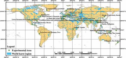
Figure 1 presents the distribution of validation data for different latitudinal zones, which include mainly North America (Puebla and Yucatan, Mexico; Lower Suwannee River basin, Florida, USA; Angmassaghik, Greenland; Boston, USA), South America (Pachachaca and Huagapo, Peru), Europe (Trondheim, Norway; Le Baget and Ariege, France; Siberia (Vladivostok), Russia; Tatras Mountain, Slovakia; Schneekoppe, Poland; Cordillera Betica and Andalusia, Spain), Africa (Alger, Rome,Tirana, Mediterranean zone, Algeria; Entebbe, Uganda), Asia (Southwest China and Guilin, China; Djakarta and Bandung, Indonesia; Calcutta, India; Manila, Philippines; Parau and Ravansar, Iran) and Oceania (Wellington, New Zealand; Bangeta Plateau, Papua New Guinea; Ocean Island). Based on the research data of different latitude belts in Figure 1, the comparison between the modeled results and other research results of different latitude belts is shown in Table 6.

Table 6. Comparison of dissolution rate results between this paper modeled results and other studies in different zones ($mm/ka$).

Experimental area	Latitudinal zone (low/mid/high)	^bTemperature (℃)	^bPrecipitation ($mm\cdot {\mathrm{a}}^{-1}$)	Other studies	$D^{\mathrm{d}}$(This paper)
Guilin, China	Low	18.61–19.86	1388.4–2658.7	26-84^(1)	38.71–46.70
Southwest, China^k	Low, Mid	14.81–16.36	919- 1290	14- 44^(2)	36.35–36.64
Siberia (Vladivostok), Russia	High	6.6	889	1–32^(3), 23^(4)	31.61
Tatras Mountain, Slovakia	Mid	4.5	910	29^(5), 35^(4)	28.80
Ocean Island	Mid	25.8	1891	70^(5), 72^(4)	72.93
Djakarta and Bandung, Indonesia	Low	24.8	2986	82^(5), 55-71^(4)	109.24
Manila, Philippines	Low	28.5	1926	78^(5), 66^(4)	100.40
Alger, Rome,Tirana, Mediterranean zone, Algeria	Mid	20.3	503	10-37^(6), 9-35^(4)	33.98
Le Baget and Ariege, France	Mid	10.1	763	73^(7), 75^(4)	35.17
Puebla and Yucatan, Mexico	Low	14	327	16^(8), 16^(4)	37.54
Pachachaca and Huagapo, Peru	Low	6.6	612	25-35^(8), 24-27^(4)	31.38
Parau and Ravansar, Iran	Mid	9.6	541	6^(8), 21^(8), 5-15^(4)	35.37
Bangeta Plateau, Papua New Guinea	Low	24.3	4758	170-190^(8), 146-248^(4)	197.02
Pomio, Jacquinot Bay, Papua New Guinea	Low	25.3	6568	370-430^(8), 340-404^(4)	400.56
Cordillera Betica and Andalusia, Spain	Mid	15.9	405	13– 27^(9), 12–19^(4)	36.56
Lower Suwannee The river basin, Florida,USA	Mid	22.6	1363	40^(10), 40^(4)	43.94
Marseille, France	Mid	17.3	486	0-10^(11),7^(4)	35.72
Ardeche’s Canyon, France	Mid	9	723	15-25^(12), 19-26^(4)	34.28
Sainte-Beaume’s Mountain, France	Mid	6.9	880	25-30^(13), 27^(4)	31.96
Schneekoppe, Poland	Mid	0	897	42^(14)	21.49
Angmassaghik, Greenland	High	2	907	40.8^(14)	24.83
Trondheim, Norway	High	5.5	1021	44.8^(14)	31.08
Boston, USA	Mid	9.5	1133	45.1^(14)	34.98
Wellington, New Zealand	Mid	12.5	1219	45^(14)	36.04
Calcutta, India	Low	26	1634	43.2^(14)	64.78
Entebbe, Uganda	Low	21	1470	43.7^(14)	41.97

References: (1) Cao et al. (2001);(2) Zeng (2017); (3) Corbel (1957); (4) Gombert (2002); (5) Lang (1977); (6) Nicod (1975); (7) Bakalowicz (1979); (8) Maire (1990); (9) Andreo Navarro (1997); (10) Denizman (1998); (11) Fabre (1980); (12) Gombert (1988); (13) Martin (1991); (14) Gombert (1994). Note GPCC First Guess Monthly Product: Global Precipitation Climatology Centre (Jan. 2013-present), Website: https://opendata.dwd.de/climate_environment/GPCC/first_guess/. Noted: According to Gombert (2002), was converted to $MPD\left(mm/ka\right)=MPD\left({\mathrm{m}}^3/k{m}^2/\mathrm{a}\right),$$V\left({\mathrm{m}}^3/\mathrm{a}\right)=MPD\left({\mathrm{m}}^3/k{m}^2/\mathrm{a}\right)\mathrm{\setminus }\mathrm{c}\mathrm{d}\mathrm{o}\mathrm{t}S\left(k{m}^2\right),$ $M\left(kg/\mathrm{a}\right)=V\left({\mathrm{m}}^3/\mathrm{a}\right)\cdot \delta \left(kg/{\mathrm{m}}^3\right)=MPD\left({\mathrm{m}}^3/k{m}^2/\mathrm{a}\right)\mathrm{\setminus }\mathrm{c}\mathrm{d}\mathrm{o}\mathrm{t}\mathrm{S}\left(k{m}^2\right)\cdot \delta \left(kg/{\mathrm{m}}^3\right),$ $R\left(kg/k{m}^2\cdot \mathrm{a}\right)=M\left(kg/\mathrm{a}\right)/S\left(k{m}^2\right)=MPD\left({\mathrm{m}}^3/k{m}^2/\mathrm{a}\right)\cdot \delta \left(kg/{\mathrm{m}}^3\right)$. The unit of $D$ is $mg\mathrm{\setminus }\mathrm{c}\mathrm{d}\mathrm{o}\mathrm{t}\mathrm{c}{\mathrm{m}}^{-2}\cdot {\mathrm{a}}^{-1}$ the results of calculation are converted into units in the paper, $D\times {\delta }^{-1}=Nmm/\mathrm{a},\delta$ is that the average specific gravity of limestone is 2500 kg/m3 (Williams 1963). Note China’s southwest region mainly includes Yunnan Province, Guizhou Province, Sichuan Province, Guangxi Province, Hunan Province, Hubei Province, and Chongqing Municipality.

As observed in Table 6, it can be found that the dissolution rate calculated in this paper is much close to the values of other dissolution rates, such as Tatras Mountain, Bangeta Plateau, Papua and Pomio, Jacquinot Bay and so on. In addition, there are some predicted values that deviate from the corresponding values of other researches, which is mainly due to the noise in the dissolution rate model. The results of Schnoor and Stumm (1990) and Swoboda-Colberg and Drever (1993) show that there are differences in predictions based on experimental research of field dynamical systems, but the differences are within the estimation error of one to two digits. For example, the difference in chemical carbonate weathering rates calculated by Gombert (2002) and Lang (1977) is 12 mm/ka in the region researched in Manila, Philippines in Table 6; and the maximum difference in carbonate chemical weathering rate calculated by Gombert (2002) and Maire (1990) in the Bangeta Plateau, Papua New Guinea research region is 58 mm/ka. Therefore, the results estimated by the dissolution rate model in this paper are within the error. It can be applied to estimate the carbonate weathering rate.

3. Estimation of the global karst carbon sink

3.1. Data sets

3.1.1. Global carbonate area data

The global carbonate data is provided by the School of Geography and Environmental Sciences at the University of Auckland, and specific information presentations can be found at https://digitalcommons.usf.edu/kip_data/137. The carbonate data were developed by Williams and Fong to distinguish between relatively pure and continuous or discontinuous carbonate regions (Williams and Fong 2007). The area data for the carbonate outcrops were obtained using GIS on the Eckert IV iso-area projection. Although not all carbonates are well karstification, most of them are prone to karstification (Williams and Fong 2007). Therefore, the carbonate outcrop area provides an upper limit to the exposed area of karst terrain. The Open Access World Karst Aquifers Map has more information on this (chen et al. 2017). Figure 2 is a comparatively new map of the World Karst Aquifers, which includes data and information on groundwater resources from the Worldwide Hydrogeological Mapping and Assessment Program (WHYMAP). The specific map data information presentation can be visited at the URL: https://www.bgr.bund.de/whymap/EN/Maps_Data/Wokam/wokam_node_en.html.

Figure 2. World Karst Aquifer Map (Chen et al. 2017).

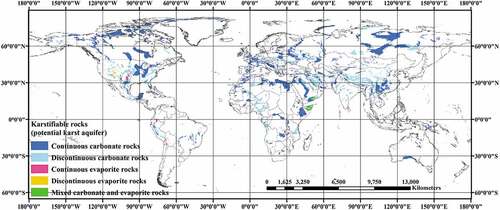
The carbonate rock types in the natural environment are mainly composed of dolomite ($\mathrm{C}\mathrm{a}\mathrm{M}\mathrm{g}(\mathrm{C}{\mathrm{O}}_3{)}_2$) and limestone ($\mathrm{C}\mathrm{a}\mathrm{C}{\mathrm{O}}_3$). Dolomite and limestone are common carbonate minerals in carbonate rocks, which are widely distributed in karst areas. The dolomite is mainly distributed in these places around the world, such as Traversella and Brosso, Piedmont, Ital; Eugui, Navarra Province, Spain; Trieben and Hall, Tirol, Austria; Freiberg and Schneeberg, Saxony, Germany; Lengenbach, Binntal, Switzerland; Trepca, Serbia, Yugoslavia; Frizington, Cumbria, England; Vuoriyarvi carbonatite complex, Kola Peninsula, Russia and so on. Specific information may be accessed at https://www.azomining.com/Article.aspx?ArticleID=279.

Since there are uncertainties in accurately distinguishing limestone (Limestone is a carbonate rock with calcite as the main component) and dolomite in global geological maps, it is assumed in this research that all carbonate outcrops are calcite.

3.1.2. Temperature and precipitation datasets

Temperature and precipitation datasets were obtained from the Climate Change Knowledge Portal (CCKP). The CCKP is an online platform that provides climate-related information, as well as data and tools. The CCKP has provided a regional and national online platform for climate change and development data. The data can be downloaded at https://climateknowledgeportal.worldbank.org/.

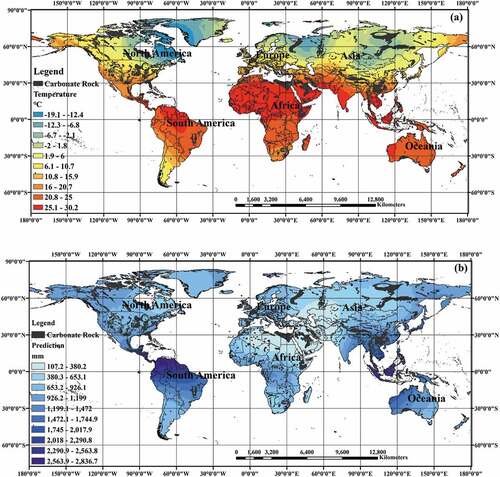
After downloaded the temperature and precipitation data from CCKP platform, this paper establishes the database by GIS technology and stores the data in the form of point data. This paper adopts spatial kriging interpolation method to process the point data and obtain the distribution map as shown in Figure 3.

Figure 3. (a) Temperature distribution map; (b) Precipitation distribution map.

3.2. Estimation of the global karst carbon sink

The basic reaction of carbonate weathering can be expressed by (Dreybrodt 1999; Liu and Zhao 2000; Yuan and Liu 2003):

(7) $CaC{O}_3+C{O}_2+{\mathrm{H}}_2\mathrm{O}\iff C{a}^{2+}+2HC{O}_3^{-}$(7)

The $C{O}_2$ are calculated by

(8) $F=D\times S\times R\times {\mathrm{M}}_{\mathrm{C}{\mathrm{O}}_2}/{\mathrm{M}}_{\mathrm{C}\mathrm{a}\mathrm{C}{\mathrm{O}}_3}$(8)

Where$F$is the result of $C{O}_2$ sink of karst action in ${10}^{10}\mathrm{g}\cdot {\mathrm{a}}^{-1}$; $D$ is the dissolution rate of rock test in $\mathrm{m}\mathrm{g}\cdot \mathrm{c}{\mathrm{m}}^{-2}\cdot {\mathrm{a}}^{-1}$; $S$ is the karst area in $\mathrm{k}{\mathrm{m}}^2$; $D$ is the carbonate purity of the rock test, i.e. $R$ = 0.97; ${\mathrm{M}}_{\mathrm{C}{\mathrm{O}}_2}$is $C{O}_2$ molecular mass, ${\mathrm{M}}_{\mathrm{C}{\mathrm{O}}_2}$ = 44; ${\mathrm{M}}_{\mathrm{C}\mathrm{a}\mathrm{C}{\mathrm{O}}_3}$is $\mathrm{C}\mathrm{a}\mathrm{C}{\mathrm{O}}_3$ molecular mass, ${\mathrm{M}}_{\mathrm{C}\mathrm{a}\mathrm{C}{\mathrm{O}}_3}$ = 100.

With Equation (8)(8) $F=D\times S\times R\times {\mathrm{M}}_{\mathrm{C}{\mathrm{O}}_2}/{\mathrm{M}}_{\mathrm{C}\mathrm{a}\mathrm{C}{\mathrm{O}}_3}$(8) , the $C{O}_2$ consumed by the global carbonate weathering can be obtained by

(9) $G_{C{O}_2}=\sum F_{C{O}_2}=4.268\times {10}^9\sum _{i=1}^n{S}_i{D}_i$(9)

Where $D_i$ is the dissolution rate of a karst area in $\mathrm{m}\mathrm{g}\cdot \mathrm{c}{\mathrm{m}}^{-2}\cdot {\mathrm{a}}^{-1}$; $S_i$ is the carbonate area of the karst region in $\mathrm{k}{\mathrm{m}}^2$.

In order to calculate the $C{O}_2$ consumed by carbonate weathering using equation (9)(9) $G_{C{O}_2}=\sum F_{C{O}_2}=4.268\times {10}^9\sum _{i=1}^n{S}_i{D}_i$(9) , we have to conduct the steps below: firstly, Kriging method was used to make spatial interpolation for temperature data and precipitation data, respectively; secondly, the temperature and precipitation values of the different carbonate regions were calculated; finally, the $C{O}_2$ consumed by carbonate weathering in the corresponding region was calculated by using the dissolution rate model. According to the geographic carbonate rock data from Williams and Fong (2007), mathematical and statistical methods were applied to arrange and visualize the karst carbon sink data in this paper, as shown in Figure 4.

Figure 4. Distribution of the $C{O}_2$ consumed by the global carbonate karstification.

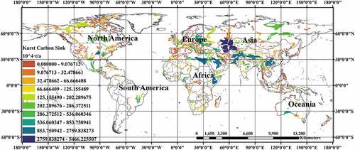
By observing Figure 4, the countries with more $C{O}_2$ consumption by carbonate karstification include the United States, Canada, Mexico, Brazil, Algeria, Turkey, Ukraine, Russia, Kazakhstan, Iran, Australia, China, and India, etc. According to the calculation results in Figure 4, we can calculate that the absorption $C{O}_2$ of the global carbonate weathering is $7.62258176\times {10}^{14}$ $\mathrm{g}\cdot {\mathrm{a}}^{-1}$ (0.208 $Gt\cdot \mathrm{C}\cdot {\mathrm{a}}^{-1}$，1 Gigatonne of Carbon (GtC) = 1 billion tons of carbon).

In addition, carbonate chemical weathering is affected by other acids in addition to the carbonic acid dissolution (Gaillardet et al. 2019). These acids are mainly sulfuric acid and nitric acid, which cause carbonate chemical weathering in nature (Spence and Telmer 2005; Calmels et al. 2007; Perrin, Probst, and Probst 2008). Sulfuric acid can be formed by the oxidation of sulfur-containing materials and the pyrite oxidative weathering after the volcanic eruption in nature, or the acid rain caused by artificial combustion of coal, and nitric acid is mainly anthropogenic, which is produced by converting ammonium into nitrate (Gaillardet et al. 2019). According to the results of research by Spence and Telmer (2005), the $C{O}_2$ released from carbonate induced by sulfuric acid can offset 48% of the $C{O}_2$ absorbed by silicate weathering. And the $C{O}_2$ of nitric acid-induced carbonate weathering release accounts for 15% $C{O}_2$ of the silicate weathering absorption in the research of nitric acid-induced carbonate weathering (Perrin, Probst, and Probst 2008). Then, the $C{O}_2$ of the two acids induced carbonate release can offset the silicate weathering to absorb 63% of $C{O}_2$. The global uptake of $C{O}_2$ from silicate weathering is 0.014 $Gt\cdot \mathrm{C}\cdot {\mathrm{a}}^{-1}$, and the $C{O}_2$ of carbonate weathering absorption in the silicate region is 0.063 $Gt\cdot \mathrm{C}\cdot {\mathrm{a}}^{-1}$ (Liu, Dreybrodt, and Liu 2011). It can be obtained that the $C{O}_2$ of these two acids induced carbonate weathering is 0.00882 $Gt\cdot \mathrm{C}\cdot {\mathrm{a}}^{-1}$ (0.014 × 63% = 0.00882 $Gt\cdot \mathrm{C}\cdot {\mathrm{a}}^{-1}$). Finally, the global carbonate karst carbon sink was estimated is approximately 0.26 $Gt\cdot \mathrm{C}\cdot {\mathrm{a}}^{-1}$ (0.208 + 0.063–0.00882 ≈ 0.26 $Gt\cdot \mathrm{C}\cdot {\mathrm{a}}^{-1}$).

3.3. The verification of global karst carbon sink and its comparative analysis

The results are compared with international estimates of karst carbon sink, and differences in the estimation of karst carbon sink in the paper are due to the different research methods and data sources applied by different researchers. Table 6 shows the global karst carbon sink estimated in this paper and the results of other researchers’ estimates of global karst carbon sink.

As observed from Table 7, it is discovered that the karst carbon sink calculated in this paper is 0.26 $Gt\cdot \mathrm{C}\cdot {\mathrm{a}}^{-1}$ in the range of 0.1 to 0.4 $Gt\cdot \mathrm{C}\cdot {\mathrm{a}}^{-1}$, which is very close to the results calculated by the researchers Gombert and Zaihua Liu. There may be several aspects that cause different estimation results: 1) The methods applied to research carbonate weathering are mainly focused on dynamic theory, chemical equilibrium and hydrological models (Romero-Mujalli, Hartmann, and Börker 2019; Beaulieu et al. 2012; Goddéris et al. 2006, 2013; Roelandt et al. 2010), and empirical relationships between runoff, temperature, and soil properties (Amiotte-Suchet and Probst 1993; Bluth and Kump 1994; Hartmann et al. 2014; Romero-Mujalli, Hartmann, and Börker 2019). Because of the differences in these methods, the fields of application are different, resulting in different results of the calculations. For example, the calculation cost of the dynamic theory method is often relatively high, which is usually applied to the local scale. The hydrogeochemical method only involves the atmospheric $C{O}_2$ consumed by carbonate rock weathering, while ignoring the “net sink” effect of silicate weathering. 2) Due to the rapid dissolution of calcite, the annual calculation of carbonate weathering is limited, which forces a change in the time step of each calculation, which significantly increases the working calculation time (Roland et al. 2013). 3) The difference between the collected data and information. There may be incomplete and data timeliness issues for collected river chemistry data. In the early global scale, these methods were mainly based on the estuary data of large rivers (Gaillardet et al. 1999; Hartmann et al. 2014), ignoring river data in small catchment areas.

Table 7. Carbon consumption of karst dissolution processes calculated by different researchers.

Author	Calculation results of karst carbon sink ($Gt\cdot \mathrm{C}\cdot {\mathrm{a}}^{-1}$)	Method
Yuan (1997)	0.61	DM
Ludwig et al. (1998)	0.096	River chemistry method
Gaillardet et al. (1999)	0.15	River chemistry method
Liu and Zhao (2000)	0.11–0.41	DBL-model, Tablet test method
Gombert (2002)	0.3	MPD
Burdige, Zimmerman, and Hu (2008)	0.1	Pore water chemical composition and advective diffusive model
Cao et al. (2016)	0.36–0.44	DM
Zhou et al. (2020)	0.095	Using $GEM-C{O}_2$ to extrapolate global karst carbon sink
This paper	0.26	RSM

In summary, the estimated karst carbon sink of 0.26 $Gt\cdot \mathrm{C}\cdot {\mathrm{a}}^{-1}$ in this paper accounts for 20% of the “missing carbon sink” of 1.3 $Gt\cdot \mathrm{C}\cdot {\mathrm{a}}^{-1}$ in the continental biosphere (Schimel et al. 1996), which is based on 10% to 30% unknown residual land carbon sink (Yuan and Liu 2003).

3.4. Trend of global karst carbon sink

To be able to understand the future changes of global karst carbon sink, temperature and precipitation data from 1951 to 2050 were collected in this paper, and equation (9)(9) $G_{C{O}_2}=\sum F_{C{O}_2}=4.268\times {10}^9\sum _{i=1}^n{S}_i{D}_i$(9) was used to estimate the global karst carbon sink from 1951 to 2050. The temperature and the precipitation data were obtained from CCKP (see Research Data for specific information), where the data from 2016 to 2050 were obtained under RCP4.5 (Representative Concentration Pathway 4.5). According to the estimation results of this century, the temperature, precipitation, and global karst carbon sink from 1951 to 2050 are counted in the paper (this paper applied Python to batch process the data from 1951 to 2050, and calculated the global karst carbon sink from 1950s to 2050s, the code is downloaded from https://www.jianguoyun.com/p/DYEIKJ4Qj9vhCRi_44cE), as shown in Figure 5.

Figure 5. Variation trend of global karst region temperature, precipitation, and karst carbon sink from 1951 to 2050.

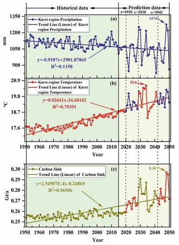
Figure 5 shows the increasing trend of temperature and karst carbon sink in the global karst region from 1951 to 2050, with annual increase values of 0.03°C·${\mathrm{a}}^{-1}$ and 2.55 × 10⁻⁴ $Gt\cdot \mathrm{C}\cdot {\mathrm{a}}^{-1}$, respectively. Whereas precipitation shows a slight decreasing trend, with an annual decrease value of 0.91 $mm\cdot {\mathrm{a}}^{-1}$. By observing Figure 5, the changes of temperature, precipitation and karst carbon sink are in a relatively stable state before 2020, while the fluctuations of temperature, precipitation and karst carbon sink are greatly changed after 2020. In particular, the fluctuation of temperature, precipitation and karst carbon sink from 2028 to 2050 has a maximum value of 20.6 °C (2034), 1274 mm (2048) and 0.30 $Gt\cdot \mathrm{C}\cdot {\mathrm{a}}^{-1}$ (2048), respectively, in which the main reason for the maximum value of karst carbon sink is that the precipitation in 2048 has increased compared with that of previous years.

By observing Figures 5(a,b), the temperature and precipitation fluctuate a lot from 2020 to 2050. This is because human activities emit a large amount of $C{O}_2$ into the atmosphere, which creates a greenhouse effect and leads to global warming. The intensity and frequency trends of certain climate and weather extreme events occur over the time span of global warming (IPCC 2018). At the same time, the karst carbon sink also shows a large fluctuation variation from 2020 to 2050 (Figure 5(c)). The main reason for the fluctuating variations in karst carbon sink can be attributed to fluctuations from temperature and precipitation. By comparing the fluctuating changes of temperature, precipitation, and karst carbon sink from 2020 to 2050, we found that Figures 5(b) and 5(c) show a positive correlation between temperature and karst carbon sink from 2020 to 2050, especially the fluctuating changes from 2020 to 2028 and 2042 to 2050 are very similar (blue band in Figure 5(b) and red band in Figure 5(c)). It is due to the strong dependence of mineral dissolution on temperature (Kump, Brantley, and Arthur 2000). Meanwhile, when comparing the variation of precipitation and karst carbon sink, the effect of precipitation on karst carbon sink is insignificant, but the fluctuation of precipitation from 2020 to 2050 affects the strength of carbon sink fluctuation due to the important dependence of mineral dissolution on the strength of hydrological cycle (Kump, Brantley, and Arthur 2000). The height variation of precipitation amplitude provides an upper limit for the amplitude height of karst carbon sink, which affects the variation of amplitude height of karst carbon sink fluctuation, for example, the maximum value of 1274 mm of precipitation appears in 2048, and the corresponding karst carbon sink will also appear the maximum value of 0.30 $Gt\cdot \mathrm{C}\cdot {\mathrm{a}}^{-1}$. Although there is an inverse trend of precipitation and karst carbon sink from 2020 to 2050, the effect of precipitation on karst carbon sink is compensated by the temperature increase that alters the concentration and transport rate of $C{O}_2$ in the chemically weathered environment of carbonate rock (Davidson and Janssens 2006; Wan et al. 2007; Zeng 2017; Liu et al. 2018).

In summary, there will be changes in the hydrological cycle facilitated by global warming through precipitation patterns and redistribution of continental vegetation, which will increase carbonate weathering (Labat et al. 2004; Liu, Dreybrodt, and Liu 2011; Liu et al. 2018; Beaulieu et al. 2012). The carbonate weathering flux between terrestrial waters and the ocean contributes to the biological carbon depletion in aquatic systems under changes in the global hydrological cycle (Riebesell et al. 2007; Liu, Dreybrodt, and Liu 2011; Liu et al. 2018), which further enhances the global karst carbon sink effect. Consequently, there are important impacts of climate change on karst carbon sink. While the change of global karst carbon sink shows not only an increasing trend in the future but also its fluctuation. This change may be related to global warming. Global warming will change the future changes of karst carbon sink through the changes in temperature and precipitation, which are manifested in the continuous increase of karst carbon sink. With this increasing karst carbon sink, which may be a considerable potential carbon sink on land, it can suppress the increasing $C{O}_2$ concentration in the atmosphere in the future and make an important contribution to the mitigation of global warming.

3.5. Further improvement of karst carbon sink estimation model

This paper proposes that the dissolution rate model constructed by response surface methodology is a mathematical regression equation. Although the important factor variables affecting karst carbon sink are employed in this paper, the research on the correlation between carbon sink fluxes caused by other land cover factors (Calmels, Gaillardet, and François 2014) requires further in-depth quantification of the estimation method of karst carbon sink fluxes. However, this method requires multiple significance tests for the parameters of the independent variables, which is a tedious and complicated step process. This is because to improve the accuracy of the response surface model requires analyzing the significance of each parameter and its combination (the independent variables of each parameter combination, such as the combination variables $TP$, $T^{2}P$, $T{P}^2$, $T^3$, $P^3$, $T^2{P}^2$, $T^{3}P$ and $T{P}^3$ in this paper) on the response, selecting the independent variables that have a significant impact on the response, and ignoring the independent variables that have little impact on the response, so as to effectively reduce the fitted coefficients of the response surface function and reduce the computational effort. In addition, the research method has not been extended to the hydrochemical runoff method due to the limitation of the quantity and quality of hydrological hydrochemical monitoring data samples. Therefore, there are at least two important works to be accomplished in the near future.

1. Research on the quantitative impact of land use on the model. It is necessary to improve and quantify the original values of land cover or annual Gross Primary Product (GPP) parameters as indicators of land use to research carbonate rock weathering rates.

2. Response surface methodology applied in the hydrochemical runoff method. Due to the limitation of the quantity and quality of hydrochemical monitoring data samples, it is necessary to investigate carbonate weathering rates in relation to the concentration of solutes (such as ${\mathrm{H}\mathrm{C}\mathrm{O}}_3^{-}$, ${\mathrm{K}}^{+}$, $\mathrm{N}{\mathrm{a}}^{+}$, $\mathrm{C}{\mathrm{a}}^{2+}$, etc.) from springs or basins.

4. Conclusions

The magnitude, variability, location, and mechanisms that have caused global karst carbon are uncertain for estimation of global Carbone skin, thus their research has been remained as a hot topic. Therefore, the response surface methodology is proposed in this paper to estimate the global karst carbon sink covering from 1950s to 2050s, and analyzes its future trend. The contributions from this paper can be summarized as follows:

1. Proposing a response surface methodology to establish a dissolution rate model for solution of the problem of unfavorable calculation of carbonate weathering rate in time. The proposed model has provided a feasibility research method for investigating the carbonate chemical weathering at global scale.

2. Establishing global surface carbonate karst carbon sink, which reaches 0.26 $Gt\cdot \mathrm{C}\cdot {\mathrm{a}}^{-1}$. This result is close to the result of 0.1 to 0.4 $Gt\cdot \mathrm{C}\cdot {\mathrm{a}}^{-1}$ and accounts for 20% of the “missing carbon sink”, which provides a basis for the research of 10%–30% of the residual terrestrial carbon sink that is not known, and is beneficial to further improve the global carbon cycle model.

3. Comparing the changes of temperature, precipitation and karst carbon sink from 1951 to 2050 globally. It is found that a great fluctuation of karst carbon sink from 2020 to 2050 has happened. The main reason for this fluctuation is due to the fluctuation of temperature and precipitation.

4. Discovering the relationship between global warming and karst carbon sink. This will cause the future change of karst carbon sink through the change of temperature and precipitation. And the global karst carbon sink in the future change situation not only shows an upward trend but also shows its fluctuating trend greatly.

The results of the global karst carbon sink were estimated in the paper, and the trend of karst carbon sink was predicted, which will help people understand the carbon cycle of the global terrestrial ecosystem, and provide a scientific basis for the rational use of energy and the formulation of environmental protection policies.

Disclosure statement

The authors declare that they have no known relevant financial and non-financial competing interests.

Data availability statement

We are grateful to the Climate Change Knowledge Portal (CCKP) for providing temperature and precipitation data, which can be downloaded at https://climateknowledgeportal.worldbank.org/. The World Karst Aquifer Map data is available for download at https://download.bgr.de/bgr/grundwasser/whymap/shp/WHYMAP_WOKAM_v1.zip. The data that support the findings of this research are available from the corresponding author upon reasonable request.

Additional information

Funding

This work is supported by the National Natural Science of China [41961065]; the Guangxi Innovative Development Grand Program [GuikeAD19254002 and GuikeAA18242048]; the Guangxi Natural Science Foundation for Innovation Research Team [2019GXNSFGA245001]; the Guilin Research and Development Plan Program [20190210-2]; the National Key Research and Development Program of China [2016YFB0502501]; the BaGuiScholars program of Guangxi and the Guangxi Key Laboratory of Spatial Information and Geomatics [19-050-11-12].

Notes on contributors

Bin Jia

Bin Jia is currently pursuing his PhD at the School of Earth Sciences, Guilin University of Technology, China. He has co-authored more than 10 academic papers. His research interests are geological remote sensing, karst carbon sink and GIS.

Guoqing Zhou

Guoqing Zhou (Senior Member, IEEE) received the Ph.D. degree from Wuhan University, Wuhan, China, in 1994. He was a researcher with the Department of Computer Science and Technology, Tsinghua University, Beijing, China, and a Post-Doctoral Researcher with the Institute of Information Science, Beijing jiaotong University, Beijing, China. He continued his research as an Alexander von Humboldt Fellow with the Technical University of Berlin, Berlin, Germany, from 1996 to 1998, and was a Post-Doctoral Researcher with The Ohio State University, Columbus, OH, USA, from 1998 to 2000. He was an Assistant Professor, an Associate Professor, and a Full Professor with Old Dominion University, Norfolk, VA, USA, in 2000, 2005, and 2010, respectively. He has authored or co-authored 10 books, seven book chapters, and more than 430 peer-refereed publications with more than 210 journal articles.

References

- Adamczyk, K., M. Prémont-Schwarz, D. Pines, E. Pines, and E. T. Nibbering. 2009. “Real-Time Observation of Carbonic Acid Formation in Aqueous Solution.” Science 326 (5960): 1690–1694. doi:10.1126/science.1180060.
- Amiotte-Suchet, P., and J. L. Probst. 1993. “Modelling of Atmospheric CO2 Consumption by Chemical Weathering of Rocks: Application to the Garonne, Congo and Amazon Basins.” Chemical Geology 107 (3–4): 205–210. doi:10.1016/0009-2541(93)90174-h.
- Amiotte-Suchet, P., and J. L. Probst. 1995. “A Global Model for Present-day Atmospheric/Soil CO2 Consumption by Chemical Erosion of Continental Rocks.” Tellus B: Chemical and Physical Meteorology 47 (1–2): 273–280. doi:10.3402/tellusb.v47i1-2.16047.
- Andreo Navarro, B. 1997. “Hidrogeologia de acuiferos carbonatados en las Sierras Blanca y Mijas.” PhD diss., Universidad de Malaga.
- Bakalowicz, M. 1979. “Contribution de la géochimie des eaux à la connaissance de l’aquifère karstique de la karutification.” PhD diss., Université Pierre et Marie Curie, Paris.
- Beaulieu, E., Y. Goddéris, Y. Donnadieu, D. Labat, and C. Roelandt. 2012. “High Sensitivity of the Continental-Weathering Carbon Dioxide Sink to Future Climate Change.” Nature climate change 2 (5): 346–349. doi:10.1038/nclimate1419.
- Berner, R. A. 1992. “Weathering, Plants, and the Long-Term Carbon Cycle.” Geochimica et cosmochimica acta 56 (8): 3225–3231. doi:10.1016/0016-7037(92)90300-8.
- Berner, R. A. 2004. The Phanerozoic Carbon Cycle: CO2 and O2. United Kingdom: Oxford University Press.
- Berner, R. A., A. C. Lasaga, and R. M. Garrels. 1983. “Carbonate-Silicate Geochemical Cycle and Its Effects on Atmospheric Carbon Dioxide Over the Past 100 Million Years.” American Journal of Science 283 (7): 641–683. doi:10.2475/ajs.283.7.641.
- Bluth, G. J. S., and L. R. Kump. 1994. “Lithologic and Climatologic Controls of River Chemistry.” Geochimica et cosmochimica acta 58 (10): 2341–2359. doi:10.1016/0016-7037(94)90015-9.
- Boeglin, J. L., J. Mortatti, and Y. Tardy. 1997. “Chemical and Mechanical Erosion in the Upper Niger Basin (Guinea, Mali). Geochemical Weathering Budget in Tropical Environment.” Comptes Rendus de L’academie des Sciences Series IIA Earth and Planetary Science 3 (325): 185–191. doi:10.1016/S1251-8050(97)88287-0.
- Bouchez, J., J. S. Moquet, J. C. Espinoza, J. M. Martinez, J. L. Guyot, C. Lagane, N. Filizola, L. Noriega, L. H. Sanchez, and R. Pombosa. 2017. “River Mixing in the Amazon as a Driver of Concentration-discharge Relationships.” Water Resources Research 53 (11): 8660–8685. doi:10.1002/2017WR020591.
- Breemen, N. V., and R. Protz. 1988. “Rates of Calcium Carbonate Removal from Soils.” Canadian Journal of Soil Science 68 (2): 449–454. doi:10.4141/cjss88-042.
- Brindha, K., and L. Elango. 2012. “Groundwater Quality Zonation in a Shallow Weathered Rock Aquifer Using GIS.” Geo-Spatial Information Science 15 (2): 95–104. doi:10.1080/10095020.2012.714655.
- Burdige, D. J., R. C. Zimmerman, and X. Hu. 2008. “Rates of Carbonate Dissolution in Permeable Sediments Estimated from Pore-water Profiles: The Role of Sea Grasses.” Limnology and Oceanography 53 (2): 549–565. doi:10.4319/lo.2008.53.2.0549.
- Calmels, D., J. Gaillardet, A. Brenot, and C. France-Lanord. 2007. “Sustained Sulfide Oxidation by Physical Erosion Processes in the Mackenzie River Basin: Climatic Perspectives.” Geology 35 (11): 1003–1006. doi:10.1130/g24132a.1.
- Calmels, D., J. Gaillardet, and L. François. 2014. “Sensitivity of Carbonate Weathering to Soil CO2 Production by Biological Activity Along a Temperate Climate Transect.” Chemical Geology 390: 74–86. doi:10.1016/j.chemgeo.2014.10.010.
- Cao, J. H., D. X. Yuan, G. X. Pan, and Y. S. Lin. 2001. “Effect of Rainfall on Soil Dynamics and Simulation of Karst Effects.” Journal of Southwest Normal University 26 (206): 13–19. In Chinese.
- Cao, J., B. Hu, C. Groves, F. Huang, H. Yang, and C. Zhang. 2016. “Karst Dynamic System and the Carbon Cycle.” Zeitschrift für Geomorphologie, Supplementary Issues 60 (2): 35–55. doi:10.1127/zfg_suppl/2016/00304.
- Chen, Z., N. Goldscheider, A. Auler, M. Bakalowicz, S. Broda, D. Drew, J. Hartmann, et al. 2017. ”World Karst Aquifer Map (WHYMAP WOKAM).” BGR, IAH, KIT, UNESCO. doi:10.25928/b2.21_sfkq-r406.
- Chen, B., R. Yang, Z. Liu, H. Sun, H. Yan, Q. Zeng, S. Zeng, C. Zeng, and M. Zhao. 2017. “Coupled Control of Land Uses and Aquatic Biological Processes on the Diurnal Hydrochemical Variations in the Five Ponds at the Shawan Karst Test Site, China: Implications for the Carbonate Weathering-Related Carbon Sink.” Chemical Geology 456: 58–71. doi:10.1016/j.chemgeo.2017.03.006.
- Cooke, R. U., R. J. Inkpen, and G. F. S. Wiggs. 1995. “Using Gravestones to Assess Changing Rates of Weathering in the United Kingdom.” Earth Surface Processes and Landforms 20 (6): 531–546. doi:10.1002/esp.3290200605.
- Corbel, J. 1957. “Les karsts du nord-ouest de l’Europe et de quelques régions de comparaison: Institut des études rhodaniennes de l’Universite de Lyon.” Mémoires et Documents 12: 541.
- Davidson, E. A., and I. A. Janssens. 2006. “Temperature Sensitivity of Soil Carbon Decomposition and Feedbacks to Climate Change.” Nature 440 (7081): 165–173. doi:10.1038/nature04514.
- Denizman, C. 1998. “Evolution of karst in the lower Suwannee River basin.” PhD diss., University of Florida.
- Detwiler, R. P., and C. A. Hall. 1988. “Tropical Forests and the Global Carbon Cycle.” Science 239 (4835): 42–47. doi:10.1126/science.239.4835.42.
- Dreybrodt, W. 1999. “Chemical Kinetics, Speleothem Growth and Climate.” Boreas 28 (3): 347–356. doi:10.1080/030094899422073.
- Dreybrodt, W., and D. Buhmann. 1991. “A Mass Transfer Model for Dissolution and Precipitation of Calcite from Solutions in Turbulent Motion.” Chemical Geology 90 (1–2): 107–122. doi:10.1016/0009-2541(91)90037-R.
- Dupré, B., C. Dessert, P. Oliva, Y. Goddéris, J. Viers, L. François, R. Millot, and J. Gaillardet. 2003. “Rivers, Chemical Weathering and Earth’s Climate.” Comptes Rendus Geoscience 335 (16): 1141–1160. doi:10.1016/j.crte.2003.09.015.
- Fabre, G. 1980. “Recherches hydrogéomorphologiques en Langedoc oriental.” PhD diss., Université d’Aix en Provence, Marseille II, Institut de Géographie.
- Fan, S., M. Gloor, J. Mahlman, S. Pacala, J. Sarmiento, T. Takahashi, and P. Tans. 1998. “A Large Terrestrial Carbon Sink in North America Implied by Atmospheric and Oceanic Carbon Dioxide Data and Models.” Science 282 (5388): 442–446. doi:10.1126/science.282.5388.442.
- Ferguson, P. R., K. D. Dubois, and J. Veizer. 2011. “Fluvial Carbon Fluxes Under Extreme Rainfall Conditions: Inferences from the Fly River, Papua New Guinea.” Chemical Geology 281 (3–4): 283–292. doi:10.1016/j.chemgeo.2010.12.015.
- Fisher, M. J., I. M. Rao, C. E. Lascano, J. I. Sanz, R. J. Thomas, R. R. Vera, and M. A. Ayarza. 1995. “Pasture Soils as Carbon Sink.” Nature 376 (6540): 473. doi:10.1038/376473a0.
- Ford, D., and P. D. Williams. 2007. Karst Hydrogeology and Geomorphology. Hoboken: John Wiley & Sons.
- Fraysse, F., O. S. Pokrovsky, and J. D. Meunier. 2010. “Experimental Study of Terrestrial Plant Litter Interaction with Aqueous Solutions.” Geochimica et cosmochimica acta 74 (1): 70–84. doi:10.1016/j.gca.2009.09.002.
- Gaillardet, J., D. Calmels, G. Romero-Mujalli, E. Zakharova, and J. Hartmann. 2019. “Global Climate Control on Carbonate Weathering Intensity.” Chemical Geology 527: 118762. doi:10.1016/j.chemgeo.2018.05.009.
- Gaillardet, J., B. Dupré, P. Louvat, and C. J. Allegre. 1999. “Global Silicate Weathering and Consumption Rates Deduced from the Chemistry of Large Rivers.” Chemical Geology 159 (1–4): 3–30. doi:10.1016/s0009-2541(99)00031-5.
- Gams, I. 1985. “International Comparative Measurement of Surface Solution by Means of Standard Limestone Tables.” Zbornik Ivana Rakovica, Razprave 4, Razrada Sazu 26: 361–386.
- Gislason, S. R., E. H. Oelkers, E. S. Eiriksdottir, M. I. Kardjilov, G. Gisladottir, B. Sigfusson, A. Snorrasond, et al. 2009. “Direct Evidence of the Feedback Between Climate and Weathering.” Earth and Planetary Science Letters 277 (1–2): 213–222. doi:10.1016/j.epsl.2008.10.018.
- Giusti, E. V. 1978. Hydrogeology of the Karst of Puerto Rico (No. 1012). Washington: US Government Printing Office.
- Godard, V., V. Ollivier, O. Bellier, C. Miramont, E. Shabanian, J. Fleury, L. Benedetti, V. Guillou, and A. Team. 2016. “Weathering-Limited Hillslope Evolution in Carbonate Landscapes.” Earth and Planetary Science Letters 446: 10–20. doi:10.1016/j.epsl.2016.04.017.
- Goddéris, Y., S. L. Brantley, L. François, J. Schott, D. Pollard, M. Deque, and M. Dury. 2013. “Rates of Consumption of Atmospheric CO2 Through the Weathering of Loess During the Next 100 Yr of Climate Change.” Biogeosciences 10: 135–148. doi:10.5194/bg-10-135-2013.
- Goddéris, Y., L. M. François, A. Probst, J. Schott, D. Moncoulon, D. Labat, and D. Viville. 2006. “Modelling Weathering Processes at the Catchment Scale: The WITCH Numerical Model.” Geochimica et cosmochimica acta 70 (5): 1128–1147. doi:10.1016/j.gca.2005.11.018.
- Gombert, P. 1988. “Hydrogéologie et karstogénèse du Bas-Vivarais calcaire (Ardèche, France).” PhD diss., Université des Sciences et Techniques du Languedoc.
- Gombert, P. 1994. “Approche théorique simplifiée de la dissolution karstique.” Karstologia 24 (1): 41–51. doi:10.3406/karst.1994.2341.
- Gombert, P. 2002. “Role of Karstic Dissolution in Global Carbon Cycle.” Global & Planetary Change 33 (1): 177–184. doi:10.1016/s0921-8181(02)00069-3.
- Gupta, H., G. J. Chakrapani, K. Selvaraj, and S. J. Kao. 2011. “The Fluvial Geochemistry, Contributions of Silicate, Carbonate and Saline–Alkaline Components to Chemical Weathering Flux and Controlling Parameters: Narmada River (Deccan Traps), India.” Geochimica et cosmochimica acta 75 (3): 800–824. doi:10.1016/j.gca.2010.11.010.
- Hartmann, J. 2009. “Bicarbonate-Fluxes and CO2-Consumption by Chemical Weathering on the Japanese Archipelago—application of a Multi-Lithological Model Framework.” Chemical Geology 265 (3–4): 237–271. doi:10.1016/j.chemgeo.2009.03.024.
- Hartmann, J., and N. Moosdorf. 2011. “Chemical Weathering Rates of Silicate-Dominated Lithological Classes and Associated Liberation Rates of Phosphorus on the Japanese Archipelago—implications for Global Scale Analysis.” Chemical Geology 287 (3–4): 125–157. doi:10.1016/j.chemgeo.2010.12.004.
- Hartmann, J., N. Moosdorf, R. Lauerwald, M. Hinderer, and A. J. West. 2014. “Global Chemical Weathering and Associated P-Release—the Role of Lithology, Temperature and Soil Properties.” Chemical Geology 363: 145–163. doi:10.1016/j.chemgeo.2013.10.025.
- Houghton, R. A., E. A. Davidson, and G. M. Woodwell. 1998. “Missing Sinks, Feedbacks, and Understanding the Role of Terrestrial Ecosystems in the Global Carbon Balance.” Global biogeochemical cycles 12 (1): 25–34. doi:10.1029/97gb02729.
- Ichikuni, M. 1976. Role of Water in Geochemical Systems. Yatazawa Noriko, Japan: University of Tokyo Press.
- Intergovernmental Panel on Climate Change (IPCC). 2018. “Summary for Policymakers of IPCC Special Report on Global Warming of 1.5°C Approved by Governments.” Accessed October 8 2019. https://www.ipcc.ch/2018/10/08/summary-for-policymakers-of-ipcc-special-report-on-global-warming-of-1-5c-approved-by-governments/.
- Jiang, B., Y. Bamutaze, and P. Pilesjo. 2014. “Climate Change and Land Degradation in Africa: A Case Study in the Mount Elgon Region, Uganda.” Geo-Spatial Information Science 17 (1): 39–53. doi:10.1080/10095020.2014.889271.
- Kitano, Y. 1984. Environmental Chemistry of the Earth. Shokabo: Kazuhiro Yoshino, Japan.
- Kump, L. R., S. L. Brantley, and M. A. Arthur. 2000. “Chemical Weathering, Atmospheric CO2, and Climate.” Annual Review of Earth and Planetary Sciences 28 (1): 611–667. doi:10.1146/annurev.earth.28.1.611.
- Labat, D., Y. Goddéris, J. L. Probst, and J. L. Guyot. 2004. “Evidence for Global Runoff Increase Related to Climate Warming.” Advances in Water Resources 27 (6): 631–642. doi:10.1016/j.advwatres.2004.02.020.
- Lal, R. 2004. “Soil Carbon Sequestration Impacts on Global Climate Change and Food Security.” Science 304 (5677): 1623–1627. doi:10.1126/science.1097396.
- Lal, R. 2007. “Carbon Sequestration.” Philosophical Transactions of the Royal Society B: Biological Sciences 363 (1492): 815–830. doi:10.1098/rstb.2007.2185.
- Lang, S. 1977. “Relationship Between World-Wide Karstic Denudation (Corrosion) and Precipitation.” Paper presented at Proceedings of the 7th International Speleological Congress, Sheffield, British, September 1.
- Liu, Z., and W. Dreybrodt. 2015. “Significance of the Carbon Sink Produced by H2O-Carbonate-CO2-Aquatic Phototroph Interaction on Land.” Science Bulletin 60 (2): 182–191. doi:10.1007/s11434-014-0682-y.
- Liu, Z., W. Dreybrodt, and H. Liu. 2011. “Atmospheric CO2 Sink: Silicate Weathering or Carbonate Weathering?” Applied Geochemistry 26: S292–294. doi:10.1016/j.apgeochem.2011.03.085.
- Liu, Z., W. Dreybrodt, and H. Wang. 2010. “A New Direction in Effective Accounting for the Atmospheric CO2 Budget: Considering the Combined Action of Carbonate Dissolution, the Global Water Cycle and Photosynthetic Uptake of DIC by Aquatic Organisms.” Earth-Science Reviews 99 (3–4): 162–172. doi:10.1016/j.earscirev.2010.03.001.
- Liu, Z., G. L. Macpherson, C. Groves, J. B. Martin, D. Yuan, and S. Zeng. 2018. “Large and Active CO2 Uptake by Coupled Carbonate Weathering.” Earth-Science Reviews 182: 42–49. doi:10.1016/j.earscirev.2018.05.007.
- Liu, Z., and J. Zhao. 2000. “Contribution of Carbonate Rock Weathering to the Atmospheric CO2 Sink.” Environmental Geology 39 (9): 1053–1058. doi:10.1007/s002549900072.
- Ludwig, W., P. Amiotte-Suchet, G. Munhoven, and J. L. Probst. 1998. “Atmospheric CO2 Consumption by Continental Erosion: Present-Day Controls and Implications for the Last Glacial Maximum.” Global and Planetary Change 16: 107–120. doi:10.1016/s0921-8181(98)00016-2.
- Mackenzie, F. T., and R. M. Garrels. 1971. Evolution of Sedimentary Rocks. New York: Norton.
- Ma, Z., E. Gray, E. Thomas, B. Murphy, J. Zachos, and A. Paytan. 2014. “Carbon Sequestration During the Palaeocene–Eocene Thermal Maximum by an Efficient Biological Pump.” Nature geoscience 7 (5): 382–388. doi:10.1038/ngeo2139.
- Maire, R. 1990. “La haute montagne calcaire(karsts. Cavités. Remplissage. Quaternaire. Paléoclimats).“ Karstologia-Mémoire 5: 219–248.
- Martin, J. B. 2017. “Carbonate Minerals in the Global Carbon Cycle.” Chemical Geology 449: 58–72. doi:10.1016/j.chemgeo.2016.11.029.
- Martin, P. 1991. “Quantification des flux carbonates exportés par les aquifères de la sainte baume (B. du Rh., Var, France) et estimation de la dissolution spécifique actuelle sur ce massif.” Travaux-Centre national de la recherche scientifique, Unité associée n. 903 (20): 25–36.
- Matsushi, Y., K. Sasa, T. Takahashi, K. Sueki, Y. Nagashima, and Y. Matsukura. 2010. “Denudation Rates of Carbonate Pinnacles in Japanese Karst Areas: Estimates from Cosmogenic 36Cl in Calcite.” Nuclear Instruments & Methods in Physics Research: Section B, Beam Interactions with Materials and Atoms 268 (7–8): 1205–1208. doi:10.1016/j.nimb.2009.10.134.
- Meierding, T. C. 1993. “Inscription Legibility Method for Estimating Rock Weathering Rates.” Geomorphology 6 (3): 273–286. doi:10.1016/0169-555x(93)90051-3.
- Mitchell, S. G., A. Matmon, P. R. Bierman, Y. Enzel, M. Caffee, and D. Rizzo. 2001. “Displacement History of a Limestone Normal Fault Scarp, Northern Israel, from Cosmogenic 36Cl.” Journal of Geophysical Research: Solid Earth 106 (B3): 4247–4264. doi:10.1029/2000JB900373.
- Moquet, J. S., A. Crave, J. Viers, P. Seyler, E. Armijos, L. Bourrel, E. Chavarri, et al. 2011. “Chemical Weathering and Atmospheric/Soil CO2 Uptake in the Andean and Foreland Amazon Basins.” Chemical Geology 287 (1–2): 1–26. doi:10.1016/j.chemgeo.2011.01.005.
- Moquet, J. S., J. L. Guyot, A. Crave, J. Viers, N. Filizola, J. M. Martinez, T. C. Oliveira, et al. 2016. “Amazon River Dissolved Load: Temporal Dynamics and Annual Budget from the Andes to the Ocean.” Environmental Science and Pollution Research 23 (12): 11405–11429. doi:10.1007/s11356-015-5503-6.
- Moulton, K. L., J. West, and R. A. Berner. 2000. “Solute Flux and Mineral Mass Balance Approaches to the Quantification of Plant Effects on Silicate Weathering.” American Journal of Science 300 (7): 539–570. doi:10.2475/ajs.300.7.539.
- Nicod, J. 1975. “Variations du dans les sols.” Paper presented at the Karst Processes and Relevant Landforms. Proc. of the Internat. Symposium on standardization of field research methods of karst denudation, Ljubljana, September 1-5.
- Nistor, M. M. 2019. “Vulnerability of Groundwater Resources Under Climate Change in the Pannonian Basin.” Geo-Spatial Information Science 22 (4): 345–358. doi:10.1080/10095020.2019.1613776.
- Noh, H., Y. Huh, J. Qin, and A. Ellis. 2009. “Chemical Weathering in the Three Rivers Region of Eastern Tibet.” Geochimica et cosmochimica acta 73 (7): 1857–1877. doi:10.1016/j.gca.2009.01.005.
- Pacheco, F., and C. H. van der Weijden. 1996. “Contributions of Water-rock Interactions to the Composition of Groundwater in Areas with a Sizeable Anthropogenic Input: A Case Study of the Waters of the Fundão Area, Central Portugal.” Water Resources Research 32 (12): 3553–3570. doi:10.1029/96wr01683.
- Pacheco, F. A. L., and C. H. Van der Weijden. 2002. “Mineral Weathering Rates Calculated from Spring Water Data: A Case Study in an Area with Intensive Agriculture, the Morais Massif, Northeast Portugal.” Applied Geochemistry 17 (5): 583–603. doi:10.1016/s0883-2927(01)00121-4.
- Perrin, A. S., A. Probst, and J. L. Probst. 2008. “Impact of Nitrogenous Fertilizers on Carbonate Dissolution in Small Agricultural Catchments: Implications for Weathering CO2 Uptake at Regional and Global Scales.” Geochimica et cosmochimica acta 72 (13): 3105–3123. doi:10.1016/j.gca.2008.04.011.
- Pitman, J. I. 1978. “Carbonate Chemistry of Groundwater from Tropical Tower Karst in South Thailand.” Water Resources Research 14 (5): 961–967. doi:10.1029/wr014i005p00961.
- Plummer, L. N., T. M. L. Wigley, and D. L. Parkhurst. 1978. “The Kinetics of Calcite Dissolution in CO2-Water Systems at 5 ℃ to 60 ℃ and 0.0 to 1.0 Atm.” American Journal of Science 278 (2): 179–216. doi:10.2475/ajs.278.2.179.
- Protz, R., M. J. Shipitalo, G. J. Ross, and J. Terasmae. 1988. “Podzolic Soil Development in the Southern James Bay Lowlands, Ontario.” Canadian Journal of Soil Science 68 (2): 287–305. doi:10.4141/cjss88-028.
- Radhakrishnan, N., and L. Elango. 2011. “Study of Influence of Terrain and Climatic Factors on Groundwater-Level Fluctuation in a Minor River Basin Using GIS.” Geo-Spatial Information Science 14 (3): 190–197. doi:10.1007/s11806-011-0530-z.
- Riebesell, U., K. G. Schulz, R. G. J. Bellerby, M. Botros, P. Fritsche, M. Meyerhöfer, C. Neill, et al. 2007. “Enhanced Biological Carbon Consumption in a High CO2 Ocean.” Nature 450 (7169): 545–548. doi:10.1038/nature06267.
- Roelandt, C., Y. Goddéris, M. P. Bonnet, and F. Sondag. 2010. “Coupled Modeling of Biospheric and Chemical Weathering Processes at the Continental Scale.” Global biogeochemical cycles 24: 2. doi:10.1029/2008gb003420.
- Roland, M., P. Serrano-Ortiz, A. S. Kowalski, Y. Goddéris, E. P. Sánchez-Cañete, P. Ciais, F. Domingo, et al. 2013. “Atmospheric Turbulence Triggers Pronounced Diel Pattern in Karst Carbonate Geochemistry.” Biogeosciences 10 (7): 7. doi:10.5194/bg-10-5009-2013.
- Romero-Mujalli, G., J. Hartmann, and J. Börker. 2019. “Temperature and CO2 Dependency of Global Carbonate Weathering Fluxes–Implications for Future Carbonate Weathering Research.” Chemical Geology 527: 118874. doi:10.1016/j.chemgeo.2018.08.010.
- Sarazin, G., and J. P. Ciabrini. 1997. “Water Geochemistry of Three Mountain Streams from Carbonate Watersheds in the Southern French Alps.” Aquatic Geochemistry 3 (3): 233–265. doi:10.1023/A:1009665608618.
- Sarmiento, J. L., and E. T. Sundquist. 1992. “Revised Budget for the Oceanic Uptake of Anthropogenic Carbon Dioxide.” Nature 356 (6370): 589–593. doi:10.1038/356589a0.
- Schimel, D., D. Alves, I. Enting, M. Heimann, F. Joos, D. Raynaud, T. M. L. Wigley, and M. J. Prather. 1996. “Radiative Forcing of Climate Change.” In Climate Change 1995: The Science of Climate Change, edited by E. Houghton, et al., 65–131. Cambridge: Cambridge University Press.
- Schnoor, J. L. 1990. “Kinetics of Chemical Weathering: A Comparison of Laboratory and Field Weathering Rates.” In Aquatic Chemical Kinetics: Reaction Rates of Processes in Natural Waters, edited by W. Stumm, 475–504. Hoboken: John Wiley & Sons.
- Spence, J., and K. Telmer. 2005. “The Role of Sulfur in Chemical Weathering and Atmospheric CO2 Fluxes: Evidence from Major Ions, δ13CDIC, and δ34SSO4 in Rivers of the Canadian Cordillera.” Geochimica et cosmochimica acta 69 (23): 5441–5458. doi:10.1016/j.gca.2005.07.011.
- Stallard, R. F. 1995. “Tectonic, Environmental, and Human Aspects of Weathering and Erosion: A Global Review Using a Steady-State Perspective.” Annual Review of Earth and Planetary Sciences 23 (1): 11–39. doi:10.1146/annurev.ea.23.050195.000303.
- Swoboda-Colberg, N. G., and J. I. Drever. 1993. “Mineral Dissolution Rates in Plot-Scale Field and Laboratory Experiments.” Chemical Geology 105 (1–3): 51–69. doi:10.1016/0009-2541(93)90118-3.
- Trudgill, S. T., H. A. Viles, R. Inkpen, C. Moses, W. Gosling, T. Yates, P. Collier, D. I. Smith, and R. U. Cooke. 2001. “Twenty-year Weathering Remeasurements at St Paul’s Cathedral, London.” Earth Surface Processes and Landforms: The Journal of the British Geomorphological Research Group 26 (10): 1129–1142. doi:10.1002/esp.260.
- Wan, S., R. J. Norby, J. Ledford, and J. F. Weltzin. 2007. “Responses of Soil Respiration to Elevated CO2, Air Warming, and Changing Soil Water Availability in a Model Old-field Grassland.” Global Change Biology 13 (11): 2411–2424. doi:10.1111/j.1365-2486.2007.01433.x.
- White, A. F., and A. E. Blum. 1995. “Effects of Climate on Chemical Weathering in Watersheds.” Geochimica et cosmochimica acta 59 (9): 1729–1747. doi:10.1016/0016-7037(95)00078-e.
- White, A. F., and S. L. Brantley. 2003. “The Effect of Time on the Weathering of Silicate Minerals: Why Do Weathering Rates Differ in the Laboratory and Field?” Chemical Geology 202 (3–4): 479–506. doi:10.1016/j.chemgeo.2003.03.001.
- White, W. B. 2002. “Karst Hydrology: Recent Developments and Open Questions.” Engineering Geology 65 (2–3): 85–105. doi:10.1016/S0013-7952(01)00116-8.
- Williams, P. W. 1963. “An Initial Estimate of the Speed of Limestone Solution in County Clare.” Irish Geography 4 (6): 432–441. doi:10.1080/00750776309555572.
- Williams, P., and Y. T. Fong. 2007. “World Map of Carbonate Rock Outcrops V3. 0. New Zealand: Aukland University.
- Xu, S., C. Liu, S. Freeman, Y. Lang, C. Schnabel, C. Tu, K. Wilcken, and Z. Zhao. 2013. “In-Situ Cosmogenic 36 Cl Denudation Rates of Carbonates in Guizhou Karst Area.” Chinese Science Bulletin 58 (20): 2473–2479. doi:10.1007/s11434-013-5756-8.
- Yuan, D. 1997. “The Carbon Cycle in Karst.” Zeitschrift Fur Geomorphologie Supplementband 37 (8): 91–102.
- Yuan, D. X., and Z. H. Liu. 2003. The Carbon Cycle and Karst Geological Environment. Beijing: Science Press.
- Zeng, S. B. 2017. “Climate change characteristics of the karst area in SW China and its impacts on karst-related carbon sink during the recent 40 years.” Master’s thesis, Southwest University.
- Zeng, S. B., Y. J. Jiang, and Z. H. Liu. 2016. “Assessment of Climate Impacts on the Karst-Related Carbon Sink in SW China Using MPD and GIS.” Global and Planetary Change 144: 171–181. doi:10.1016/j.gloplacha.2016.07.015.
- Zhang, J., Q. Hu, Y. Li, H. Li, and J. Li. 2021. “Area, Lake-Level and Volume Variations of Typical Lakes on the Tibetan Plateau and Their Response to Climate Change, 1972–2019.” Geo-Spatial Information Science 24 (3): 458–473. doi:10.1080/10095020.2021.1940318.
- Zhou, G., J. Huang, X. Tao, Q. Luo, R. Zhang, and Z. Liu. 2015. “Overview of 30 Years of Research on Solubility Trapping in Chinese Karst.” Earth-Science Reviews 146: 183–194. doi:10.1016/j.earscirev.2015.04.003.
- Zhou, G., B. Jia, X. Tao, and H. Yan. 2020. “Estimation of Karst Carbon Sink and Its Contribution to CO2 Emissions Over a Decade Using Remote Sensing Imagery.” Applied Geochemistry 121: 104689. doi:10.1016/j.apgeochem.2020.104689.