Estimating China’s poverty reduction efficiency by integrating multi-source geospatial data and deep learning techniques

ABSTRACT

Poverty threatens human development especially for developing countries, so ending poverty has become one of the most important United Nations Sustainable Development Goals (SDGs). This study aims to explore China’s progress in poverty reduction from 2016 to 2019 through time-series multi-source geospatial data and a deep learning model. The poverty reduction efficiency (PRE) is measured by the difference in the out-of-poverty rates (which measures the probability of being not poor) of 2016 and 2019. The study shows that the probability of poverty in all regions of China has shown an overall decreasing trend (PRE = 0.264), which indicates that the progress in poverty reduction during this period is significant. The Hu Huanyong Line (Hu Line) shows an uneven geographical pattern of out-of-poverty rate between Southeast and Northwest China. From 2016 to 2019, the centroid of China’s out-of-poverty rate moved 105.786 km to the northeast while the standard deviation ellipse of the out-of-poverty rate moved 3 degrees away from the Hu Line, indicating that the regions with high out-of-poverty rates are more concentrated on the east side of the Hu Line from 2016 to 2019. The results imply that the government’s future poverty reduction policies should pay attention to the infrastructure construction in poor areas and appropriately increase the population density in poor areas. This study fills the gap in the research on poverty reduction under multiple scales and provides useful implications for the government’s poverty reduction policy.

KEYWORDS:

• Poverty reduction efficiency (PRE)
• driving forces
• multisource big data
• deep learning
• random forest (RF)

1. Introduction

Poverty has been a major issue influencing human development (Gillis, Shoup, and Sicat 2001; Xu et al. 2019; Nili 2019). Existing literature on the assessment of poverty mainly focus on the identification of poor areas (Wang and Qian 2017; Li et al. 2019) and the evaluation of a specific poverty reduction policy in a small area (Harrison and Schipani 2007; Pratesi and Salvati 2016; Mahadevan, Amir, and Nugroho 2017). The data are mainly based on administrative data and sampling questionnaires (Clark, D’Ambrosio, and Ghislandi 2016; Ram 2011), which are costly and are time-consuming. Due to the privacy and data protection policy, such data is usually provided with low spatial resolution. Also, due to the lack of data and models, it is difficult to evaluate the regional differences in, scale effects of and driving factors of a certain country’s progress in poverty reduction (Alkire, Roche, and Vaz 2017). With the development of big data and deep learning technology, it is now possible to mine the deep spatial semantic features of multi-source geospatial data, which have been widely used to assess regional economic growth (Chen and Gao 2017; Xu et al. 2016). At present, multi-source geospatial data has been widely used in various city-related studies, such as urban land use (Liu et al. 2017; Liang et al. 2021; Yao et al. 2021), urban community exploration (Papadopoulos et al. 2012; Yue et al. 2019), urban population investigations (Kang et al. 2012; Patel et al. 2017), and urban structure analysis (Sevtsuk and Ratti 2010). Therefore, evaluating regional poverty reduction under multiple scales based on multi-source geospatial data can be a promising solution that fills the above research gaps.

Since the reform and opening up, China has made many achievements in reducing poverty and made outstanding contributions to the world’s poverty reduction efforts (Ravallion and Chen 2004). According to the latest report, the number of people living in poverty in China dropped from 98.99 million at the end of 2012 to 5.51 million at the end of 2019, with the incidence of poverty dropping from 10.2% to 0.6% (CGTN 2020). However, regional differences in China’s progress in poverty reduction and its scale effect are still unknown (Bu 2015). Therefore, the evaluation of the progress in poverty reduction and the analysis of its driving forces in China under multiple scales have both theoretical and practical significance. First, it contributes to existing literature by integrating multi-source geospatial data and deep learning techniques to examine the poverty reduction policy in the Chinese context. Second, it also provides valuable policy implications regarding how to implement efficient policy interventions in different regions in China.

This study uses a Long Short-Term Memory (LSTM) network and Random Forest (RF) model to construct the prediction model of China’s out-of-poverty rate (reflecting the wealth of an area at a given time, 0 = absolute poverty area; 1 = absolute rich area). This model predicts the out-of-poverty rate based on Real-time Tencent User Density (RTUD) and official statistics data. Using the out-of-poverty rate difference between 2016 and 2019, we also map the poverty reduction efficiency (PRE) and analyze its driving forces under multiple scales.

2. Related works

2.1. Identification of poor areas and analysis of PRE

There have been many studies on poverty identification (Alkire and Foster 2011; Foster, Greer, and Thorbecke 2010; Pokhriyal and Jacques 2017; Wagle 2002) such as the measurement of multidimensional poverty using extensions of traditional methods based on administrative data (Alkire and Foster 2011) and the identification of rural poverty (Benjamin, Brandt, and Giles 2009; Deller 2010; Li et al. 2015). The research on poverty reduction efficiency started from the debate and evaluation of the Johnson administration’s “War on Poverty” project in the 1960s in the United States (Patton, Sawicki, and Clark 2015). As poverty reduction methods were innovated, the research on poverty reduction efficiency, such as investigating the contribution of tourism (Mayer et al. 2010; Zarandian et al. 2016) and finance (Santeramo et al. 2016) to poverty reduction efficiency and microscale research from the perspective of an industrial chain (Harrison and Schipani 2007), also increased. Previous studies mainly use the Data Envelope Approach (DEA) and Geographic Information System (GIS) method to study the contributions of tourism and finance to poverty reduction efficiency (Long, Du, and Zhou 2015).

2.2. China’s economic growth and the “Hu Huanyong Line”

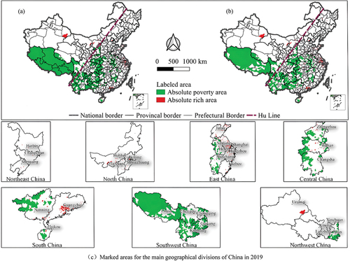
As shown in Figure 1, Hu Huanyong Line (Hu Line) is an imaginary line that stretches from Heihe (a northern Chinese city near the Russian border) to Tengchong (a southwestern Chinese city on the border with Myanmar) (Hu 1935). The Hu Line, the boundary of China’s population and urbanization development, divides China into rapidly urbanized areas with dense populations in the east and slowly urbanized areas with sparse populations in the west, which directly reflects the characteristics of China’s development (Chen et al. 2016, 2019; Huanyong 1990). Research on the Hu Line has become a hotspot since 2014 when China’s government has announced that improving the equity in the development of both sides of the Hu Line is one of its priorities (Chen et al. 2016). Existing studies mainly use qualitative methods to analyze the population distribution and urban development on both sides of the Hu Line (Chen et al. 2016; Ge and Feng 2010; Qi, Liu, and Zhao 2015; Qi et al. 2016; Wu and Wang 2008). However, few studies conducted quantitative analysis of the progress in the poverty reduction on both sides of the Hu Line or the spatial displacement of the Hu Line, which is essential for making poverty reduction policy.

Figure 1. The marked areas at the township scale in China’s mainland and the markings of various areas in China’s mainland in 2019, including the absolute poverty areas (in green color) and the absolute rich areas (in red color). (a) Spatial distribution of the marked areas in 2019. (b) Spatial distribution of the marked areas in 2016. (c) Spatial distribution of the marked areas for the main geographical divisions of China in 2019.

2.3. Multi-source geospatial data and socioeconomic study

With the development of big data technology, multi-source geospatial data have become a promising data source for reflecting users’ economic activity due to its advantages of large sample sizes and detailed information coverage of geospatial data (Azar et al. 2013; Blumenstock 2016; Montjoye et al. 2018; Hargreaves and Watmough 2021; Wang et al. 2022). Existing studies show that geospatial data can reflect and describe economic activities from multiple scales and perspectives with high accuracy (Liu et al. 2015). Mobile terminals such as mobile phone and car mobile service can generate user’s dynamic location information (Modegi 2009). Based on the geospatial data generated by mobile terminals, a large number of studies have been conducted on urban functional zoning, commercial site selection and urban work-residence balance (Chen et al. 2017; Yao et al. 2019; Zhou, Yeh, and Yue 2018). Therefore, multi-source geospatial data can be effectively used for socioeconomic research.

2.4. Deep learning and socioeconomic information extraction

Thanks to the continued improvements in computing power, deep learning methods have been developed and made great achievements in data mining (LeCun, Bengio, and Hinton 2015). Currently, many studies are using deep learning to extract information from images and further apply it to investigate the composition of the population (Gebru et al. 2017) and identify poor areas (Jean et al. 2016), but such method has high requirements on the sample size of the data. Some studies also use deep learning technology to obtain fine-scale housing price data (Yao et al. 2018) or mine the out-of-poverty rate of urban residents based on housing price data (Guan et al. 2020). The extensive application of deep learning in data information extraction and the behavioral simulation of residents provide new approaches for poverty research, and have achieved high prediction performance (Hu et al. 2022; Puttanapong et al. 2022). However, due to the complexity of the algorithm, relevant techniques have not been widely used in the research of poverty estimation or poverty reduction.

3. Study area and data

The study area of this study is China’s mainland (No statistics for Hong Kong, China, Macau, China and Taiwan, China), including 31 provincial administrative regions, 336 city administrative regions, 2819 county administrative regions, and 41,263 township administrative regions. Following the economic data released by the government (http://cpadis.cpad.gov.cn/cpad/), this study marks the absolute poverty areas and absolute out-of-poverty (rich) areas in China at the township scale (the absolute out-of-poverty areas were marked as 1 and the absolute poverty area were marked as 0). Finally, a total of 7335 absolute poor areas and 1094 absolute out-of-poverty areas were marked in 2016, and a total of 6260 absolute poor areas and 1094 absolute out-of-poverty areas were marked in 2019. The study areas are shown in Figure 1.

The data used in this study includes social media data and multi-source geospatial data. The multi-source geospatial data used in this paper include night light data, basic geographic data, traffic data, air pollution data, etc. (see Figure 2). There are 16 kinds of multi-source geospatial data with a unified resolution of $1\mathrm{k}\mathrm{m}\times 1\mathrm{k}\mathrm{m}$. All data were normalized, ranging from 0 to 1. Among these types of data, night light data can provide richer geographic information (Donaldson and Storeygard 2016) that reflects the level of economic activity to some extent (Sutton and Costanza 2002). The basic geographic data include the slope data for each region of the country, which reflects the physical geographical conditions of the study area. The traffic data include the national highway network density, the railway network data, and the national high-speed railway network data, which reflect the transportation convenience in the study area. Air pollution data mainly include the PM2.5 (fine particulate matter with a diameter of 2.5 $\mathrm{m}\mathrm{u}\mathrm{m}$ or less) concentration level, which can be used to represent the local industrial development level (Zhang et al. 2018). The above data sources are shown in Table 1.

Figure 2. Geospatial datasets: (a) Nighttime Light Index (NLI). (b) Population Density (PD). (c) Terrain Slope Value (TSV). (d) Distance to the Provincial Capital City (DPCC1). (e) Distance to the Prefectural City Center (DPCC2). (f) Distance to the County Center (DCC). (g) Distance to the Nearest High-speed Railway (DNHSR). (h) Distance to the Nearest Railway (DNR). (i) Distance to the Nearest High-speed Railway Station (DNHSRS). (j) Distance to the Nearest Railway Station (DNRS). (k) Distance to the Nearest Main Road (DNMR). (l) Road Network Density (RND). (m) January PM2.5 concentration (PM2.5_1). (n) Annual PM2.5 concentration (PM2.5_7). (o) July PM2.5 concentration (PM2.5). (p) Distance to Major Ports (DNMP).

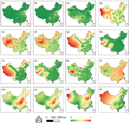
Table 1. Data sources.

Data	Format	Year	Resolution	Source
List of poor counties and rich counties	Txt	2016、2019	\	http://cpadis.cpad. gov.cn/cpad/
Traffic data	Shp	\	\	http://openstreetmap.org
Night light data	GeoTiff	2000–2012	$1\mathrm{k}\mathrm{m}\times 1\mathrm{k}\mathrm{m}$	https://ngdc.noaa.gov/
PM2.5	GeoTiff	2016	$30\mathrm{m}\times 30\mathrm{m}$	http://www.weather.com.cn/
DEM	GeoTiff	\	$30\mathrm{m}\times 30\mathrm{m}$	https://www.gscloud.cn/
Population data	Txt	2010	\	http://www.stats.gov.cn/

In this study, social media data were used to simulate population changes in various regions of China. Social media data in this study refers to The Real-time Tencent User Density data in 2016 and 2019, which was collected through the Application Programming Interface (API) provided by the Tencent EasyGo application (http://easygo.qq.com), which is the most widely used social media service provider in China. Based on the findings of Deville et al. (2014), a specific function can be used to calculate the population data within the region based on the social media data. By combing the census and social media data, we calculated the coefficients in the function proposed by Deville et al. (Deville et al. 2014; Guan et al. 2022). In this way, the population data at the current moment can be calculated based on the social media data. After the above process, RTUD data is obtained. The RTUD data includes the 24-hour average user density in three different periods including weekends, workdays and legal holidays in China’s mainland at a resolution of $1\mathrm{k}\mathrm{m}\times 1\mathrm{k}\mathrm{m}$ RTUD. Previous studies show that Tencent users account for more than 90% of the total Chinese population (Yao et al. 2017, 2022). Social media data can reflect complex human behavior and human interaction within the city, which can be good indicators for measuring political, economic, commercial and other cultural characteristics of a city (Barbier and Liu 2011; Guan et al. 2022). It also has the merits of being the big data which is superior in volume, velocity, and variety (Goodchild 2013), and makes up for the defect of traditional remote sensing images which cannot provide information of human flows (Levin, Kark, and Crandall 2015). Hence, these data can reasonably depict the behavioral and activity characteristics of the users and have been widely used for different kinds of research (Chen et al. 2018; Huang, Li, and Zhang 2019; Yao et al. 2017).

4. Method

This study uses Tencent social media data and two waves of poverty data to predict the distribution of PRE at country level, and evaluate the driving forces of PRE. Our proposed model is as follow:

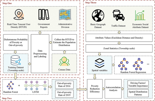
First, we build up an algorithm combining both LSTM and RF (LSTM-RFA) for predicting PRE:1. We cleaned up the raw data and tagged all targeted areas (0 = absolute poverty area; 1 = absolute rich area) based on government’s economic statistics data;2. RTUD was collected for simulating population distribution. Then, it was adjusted based on census data; 3. The tagged data was integrated with RTUD to make a semi-supervised spatio-temporal RTUD data base;4. LSTM was applied to semi-supervised spatio-temporal RTUD data base for dimensionality reduction. Then, after combing the results of LSTM model with tagged data, we used RF model to calculate two waves of out-of-poverty rate for targeted areas.

Second, we calculated the PRE based on the difference in two waves of out-of-poverty rate, and used multi-source geospatial data as predictors to examine the driving forces of PRE based on RF model. The weights of different predictors can be used for the modification of future policy and improving PRE in China.

The method flowchart of this study is shown in Figure 3. It illustrates the PRE was evaluated based on multi-period Tencent time series population data and deep learning.

Figure 3. Workflow diagram.

4.1. Constructing the out-of-poverty rate prediction model

The out-of-poverty rate prediction is the premise of the PRE evaluation. The data required for out-of-poverty rate prediction models were the RTUD and marked data for rich and poor regions. The principle of this method was to construct a semisupervised model based on the marked data and extract the economic characteristics of the targeted population based on the spatiotemporal attributes of the RTUD. The poverty fitting procedure was divided into two parts: pretreating the time-space dimension of the RTUD and the construction of the poverty fitting model based on LSTM and the RF.

The purpose of pretreating the time-space dimension of the RTUD is to ensure the spatial and temporal accuracy of the fitting. First, we conducted coordinate correction, data cleaning, mean spatial filtering and time-dimensional compression (up to 1 hour) on the original RTUD data (Chen et al. 2017). Then, the preliminary data were obtained through the zonal statistics at the district scale and kilometer grid scale. Finally, the population size and age structure of the preliminary data were corrected to the near-real population based on the 2010 national census data (Yao et al. 2018). In addition, the RTUD semisupervised spatiotemporal data were formed by associating it with the rich and poor marked data.

The role of this model is to mine high dimensional population distribution characteristics and their socio-economic attributes from RTUD data. This model constructs two LSTM layers and a fully connected layer, which reduces the time dimension of the RTUD semisupervised spatiotemporal data to extract the high-dimensional semantics of the hyperpopulation distribution. Then, the temporal features of high-dimensional semantics were classified by the RF, that is, the dichotomous probabilities of poverty or out-of-poverty were calculated.

Compared with the traditional Recurrent Neural Network (RNN), LSTM effectively solves the vanishing gradient problem in RNN training (Hochreiter and Schmidhuber 1997). LSTM has been widely used in studies related to time series data (Vlachas et al. 2018). The internal operation structure of LSTM is shown in Figure S1. RF is a combination algorithm based on classification and regression decision trees (Breiman 2001). A large number of theoretical and empirical studies have proved that the RF has high classification accuracy (Fernández-Delgado et al. 2014).

4.2. Defining the PRE and spatial analysis

In this study, the out-of-poverty rate of each region was predicted based on the out-of-poverty rate prediction model, and the difference between the predicted probability values in 2019 and 2016 was used as the poverty reduction efficiency of the local out-of-poverty rate to measure the PRE of each local region. To better reflect the out-of-poverty rates of regions with different population densities and highlight the impact of the population size (Ren 2018), this study calculated the poverty reduction efficiency of the average out-of-poverty rate of each region by taking the number of permanent residents in each region as the weight. Formulas (1) and (2) respectively represent the calculation methods of the PRE and weighted average PRE.

(1) $T=P_{2019}-P_{2016}$(1)

(2) $\stackrel{-}{T}=\frac{{\sum }_{i=1}^n{T}_i{W}_i}{{\sum }_{i=1}^n{W}_i}$(2)

Where $T$ is PRE, $\bar{T}$ is weighted average PRE, $P_{2016}\hspace{0.17em}$and$\hspace{0.17em}{P}_{2019}$ is out-of-poverty rate in 2016 and 2019, respectively. $T_i$ and$\hspace{0.17em}{W}_i$ is the PRE and population in region $i$, respectively.

This study analyzes the spatial distribution and statistical characteristics of the PRE in China at the provincial, municipal, county and district scales. To better describe the spatial distribution of the average poverty reduction efficiency, Moran’s I index, the Getis-Ord Gi* index and the Local Indicators of Spatial Association (LISA) were introduced in this study. Moran’s I index is mainly used to measure the spatial correlation of the attributes in the whole research area (Moran 1950) while the LISA index can measure the spatial correlation between each region and its adjacent areas. The Getis-Ord Gi* index was used to describe the high and low value aggregation of the targeted attributes in the local space (Ord and Getis 1995).

4.3. Mining the driving factors of the PRE based on the random forest

The multisource spatial big data used in this study involved data on the physical geography, social economy, night light data, traffic data, air pollution data, etc. Based on the spatial variables obtained above, we then adopted the method of zonal statistics to obtain the mean values of spatial variables in different regions. The RF performs well in dealing with fitting problems (Ouedraogo, Defourny, and Vanclooster 2019), which can better avoid overfitting phenomenon and provide a better explanation for variables (Breiman 2001). Currently, the RF has many applications in socioeconomic fields, such as electricity consumption prediction (Wang et al. 2018) and land use classification (Belgiu and Drăguţ 2016). In this study, the values of each spatial factor were taken as the independent variables, and the RF fitting function was used to fit the PRE. The social media data used in this study are raster data with a resolution of $1\mathrm{k}\mathrm{m}\times 1\mathrm{k}\mathrm{m}$, and each pixel value represents the average user density of this range at the current time. The study extracted the high-dimensional semantics of population distribution corresponding to each pixel in social media data based on LSTM as the input of the model, and used the tagged pixel value (rich and poor) as the output of the model to serve as the data set required by the subsequent algorithm. Pearson’s R was used to identify the influence of each spatial factor on the PRE, and the weight of each spatial factor after fitting was used to represent the extent of its impact on the PRE.

5. Results

5.1. Results of the distribution of the multiscale PRE

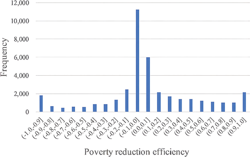
In this study, the difference between the predicted values of the model in 2019 and 2016 was taken as the poverty reduction efficiency, representing PRE; and the PRE frequency histogram was obtained, as shown in Figure 4. The statistical results show that the population-weighted average PRE is 0.264 in China. The positive average PRE indicates that China’s overall progress in poverty reduction from 2016 to 2019 is significant. However, district level statistical areas with negative PREs account for 50.167% of all the research areas, which indicates that there are also regional differences and inequity in the progress in poverty reduction in China.

Figure 4. Frequency histogram of the PREs of various regions in China at the country scale.

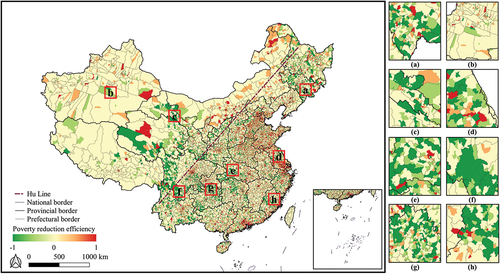
In this study, the spatial distribution of the PRE was studied on multiple scales, and the results on the provincial, municipal and county scales are shown in Figure S2, Figure S4 and Figure S5, respectively. The results show that the PRE was high in coastal provinces and North China but low in Northeast and Southwest China. Figure 5 shows the distribution of PRE at a district level. The PRE on the district scale can directly reflect the effect of governments’ poverty alleviation strategies since most of the governments’ poverty alleviation strategies are conducted and evaluated at this scale (Zhou et al. 2018; Zhou, Guo, and Liu 2019). The PRE decreased gradually from east to west, and the spatial heterogeneity is obvious. The PRE at the district level was high in eastern China but low in southwestern China. The areas with low PRE were mainly in southern Jilin, western Hubei, northern Guizhou, western Sichuan and southwestern Qinghai Provinces. Hence, the areas with low PREs were mainly in major urban agglomerations, such as the Beijing-Tianjin-Hebei urban agglomeration, the Yangtze River Delta urban agglomeration, the Guangdong-Hong Kong-Macao Greater Bay Area, the Chengdu-Chongqing urban agglomeration, the Yangtze River urban agglomeration, the Zhongyuan urban agglomeration, and the Guanzhong Plain urban agglomeration.

Figure 5. Distribution map of the PREs of counties and districts. (a) southeastern Jilin Province, (b) central Xinjiang Uygur Autonomous Region, (c) northwestern Gansu Province, (d) northern Jiangsu Province, (e) western Hubei Province, (f) southern Sichuan Province, (g) northern Guizhou Province, and (h) northwestern Fujian Province.

5.2. Spatial autocorrelation analysis of the PRE

To better understand the spatial autocorrelation of the PRE of each district, this study conducted local autocorrelation analysis on the PREs of all districts in the study area and obtained a local spatial autocorrelation statistical table (Table S3). The statistical results show that at 95% confidence, most areas in China were LL (low value cluster) type or HH (high value cluster) type. The local spatial autocorrelation map is shown in Figure 6.

Figure 6. Distribution map of the spatial autocorrelation types of the PREs in various regions of China at the township scale. HH: High-high type, high value cluster; HL: High-low type, high values neighboring surrounded by low values; LH: Low-high type, low values surrounded by high neighboring values; and LL: Low-low type, low value cluster.

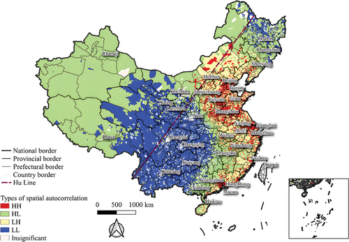
As shown in Figure 6, the autocorrelation types on the whole show an HH-LH-HL-LL transition from the southeast to the southwest. The HH type research areas were mainly distributed in the northwestern, northern and coastal regions in northern China while the LL type research areas were primarily distributed in the southwestern, central and northeastern China.

In general, most of East and South China were HH type, among which the mean values of the local spatial autocorrelation indexes in Shanghai, Shenzhen and Guangzhou were positive, and the z values representing the degrees of aggregation were 35.040, 40.059 and 28.175, respectively. The PREs of the local spatial autocorrelation indexes of these three cities were high while the PREs of the local spatial autocorrelation indexes of their surrounding cities were also high. These results indicate that these three cities may share their resources with surrounding areas (Du et al. 2020; Han and Liu 2018; Yu et al. 2018) and have positive influences on their progress in poverty reduction. In addition, Wuhan, Zhengzhou and Nanchang Provinces in Central China were each promoted a “National Central City” and get more abundant resources; therefore, they can help their surrounding areas in poverty reduction (Fang and Sun 2015; Xia et al. 2019), which makes them and their surrounding areas HH types. Hence, large cities in the southeastern and northern China and their surrounding areas were HH types since they have been developing for a long time and have frequent population and resource flows with surrounding areas (Hui et al. 2020; Wang and Song 2006).

However, the major cities in northeastern and southwestern China were HH types while their surrounding areas were LL types. This is because the major cities in Southwest China mainly attract the surrounding areas’ populations and resources to promote their own development, which has a negative influence on their progress in poverty reduction.

5.3. The out-of-poverty rate distributions of China in 2016 and 2019

The out-of-poverty rate prediction model was used to predict the out-of-poverty rates of all regions in China, and the results were plotted as shown in Figures 7 and 8. The poorest regions in China were mainly located in the southwest, the northeast, the west of the southeast and the north of the central region. The regions with the highest out-of-poverty rates in China were mainly distributed in the northern part of the North China Plain, the Bohai Sea urban agglomeration, the Yangtze River Delta, the Pearl River Delta, the Sichuan Basin, the southeastern coastal areas and the major capital cities.

Figure 7. Township scale distribution of the out-of-poverty rate in 2016 (0 equals absolute poverty and 1 equals absolute rich). (a) Beijing, the capital of China. (b) Shanghai, the richest city of China, located in the east of China. (c) Guangzhou, the center city of the Pearl River Delta, one of the richest areas of China, located in the south of China. (d) Chengdu, an important high-tech industrial base of China, located in the southwest of China. (e) Wuhan, the center city of Central China. (f) Zhengzhou, the center city of the Central Plains City Group. (g) Shenyang, the capital of Liaoning Province, located in the northeast of China. (h) Xining, the capital of Qinghai Province, located in the northwest of China.

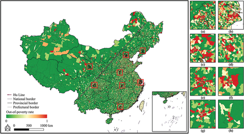
Figure 8. Township scale distribution the of out-of-poverty rate in 2019. (a) Beijing, (b) Shanghai, (c) Guangzhou, (d) Chengdu, (e) Wuhan, (f) Zhengzhou, (g) Shenyang, (h) Xining.

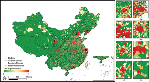
By comparing the distributions of the out-of-poverty rates among different regions in China in 2016 and 2019, it can be found that there were more areas with a high out-of-poverty rate to the east and less to the west of the Hu Line. On the west side of the Hu Line, the out-of-poverty rate decreased; while on the east side of the Hu Line, the out-of-poverty rate increased. In 2019, almost all of the regions with high out-of-poverty rates appeared on the east side of the Hu Line, indicating a significant concentration of regions with the out-of-poverty rate in eastern China.

This study further used gravity analysis to investigate the changes in the center of gravity of the out-of-poverty rate (Fang et al. 2018; Yang and Grigorescu 2017), and the results are shown in Figure 9 and Table 2. The results show that the center of gravity of China’s out-of-poverty rate was located in the southwest of Henan Province in 2016 and in the east of Henan Province in 2019, moving 105.786 km to the northeast from 2016 to 2019. This result indicates that the gap between the two sides of the Hu Line has been further widened.

Figure 9. The change of standard deviation ellipse and centroid of out-of-poverty rate between 2016 and 2019 in China.

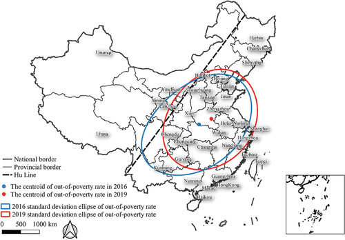
Table 2. The centroid of the out-of-poverty rate distribution and the distribution direction index.

	Centroid longitude	Centroid latitude	Ellipse direction angle	Length increase of ellipse minor axis	Length increase of ellipse major axis
2016	111.844°	32.651°	65.526°	5.774%	$-$13.924%
2019	114.501°	33.340°	62.555°

Compared with 2016, the standard deviation ellipse of the out-of-poverty rate moved 3 degrees away from the Hu Line. The increase of the short-axis length of the standard deviation ellipse of the out-of-poverty rate indicates that the overall out-of-poverty rate increased; meanwhile, the decrease of the ellipticity of the standard deviation indicates that although increasingly more regions are becoming regions with high out-of-poverty rates, the regions with high out-of-poverty rates are become more concentrated in the east.

5.4. Fractional differential for image enhancement analysis

In this study, we investigated the association between multisource spatial attributes and the PRE in China, and the results are shown in Table 3. There were 6 attributes positively correlated with the PRE, including PM2.5, PM2.5_7, PM2.5_1, PD, NLI and RND. This indicates that the degree of industrialization, population size, population activity level, economic activity, and transportation convenience are positively associated with poverty reduction. Among all the attributes, the correlation between the night light index and the PRE is the strongest, indicating that the levels of social and economic activity of residents contribute most to poverty reduction in China, and this should be highlighted in poverty alleviation policies. Hence, DCC, DNMP and TSV were negatively correlated with the PRE, indicating that the distance to the county center and the nearest port and the physiographic conditions may prevent a region from lifting itself from poverty.

Table 3. Weights and correlation coefficients of the different attributes of the PRE (a positive value indicates a positive correlation between the driver and PRE, while a negative value indicates a negative correlation; the higher the value, the stronger the correlation).

Attributes	Weights	Attributes	Weights
DNMR	$-$0.024	PM2.5	$+$0.048
RND	$+$0.025	TSV	$-$0.052
DNR	$-$0.032	PM2.5_7	$+$0.052
DNRS	$-$0.033	PM2.5_1	$+$0.057
DNHSR	$-$0.033	DNMP	$-$0.058
DNHSRS	$-$0.034	DCC	$-$0.059
DPCC2	$-$0.040	PD	$+$0.109
DPCC1	$-$0.042	NLI	$+$0.304

In this study, we further investigated the association between the multisource spatial attributes and the PRE for each province and the results were shown in Figure 10. The weights of NLI and PD were relatively high in all provinces, suggesting that the intensity of socioeconomic activity (Huang et al. 2021) and the population density (Henderson 2003) were positively associated with the PRE in most provinces. We then focused on the top 3 provinces (Shanghai, Beijing and Jiangsu Provinces), which are most influenced by NLI and PD; and found that they had the highest PREs. The average PREs of these three provinces were all higher than 0.4 and were 2.157 times the national average.

Figure 10. The weight map of the factors related to the PRE of each province in China. (NLI: Nighttime light index. PD: Population density. TSV: Terrain slope value. DPCC1: Distance to the provincial capital city. DPCC2: Distance to the prefectural city center. DCC: Distance to the county center. DNHSR: Distance to the nearest high-speed railway. DNR: Distance to the nearest railway. DNHSRS: Distance to the nearest high-speed railway station. DNRS: Distance to the nearest railway station. DNMR: Distance to the nearest main road. RND: Road network density. PM2.5_1: January PM2.5 concentration. PM2.5_7: Annual PM2.5 concentration. PM2.5: July PM2.5 concentration. DNMP: Distance to major ports.).

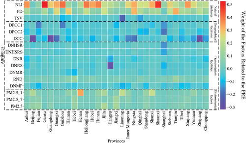
Figure 10 shows that marine ports have a strong influence on Liaoning Province among the three northeastern provinces of China, which is related to the province’s main marine ports in Northeast China. The impact of DNMP on Liaoning Province’s PRE is $-$0.105; while for Jilin and Heilongjiang, their average DNMP weights only reached $-$0.018 and $-$0.046, respectively. The average PD weight of Heilongjiang, Jilin, and Liaoning Provinces (0.170) is 30.769% higher than the national average (0.130). The results confirmed the low population density and population loss in Northeast China (Shanxi Statistical Information Network 2011), which significantly slowed down the poverty reduction rate in Northeast China and even caused economic regression.

The average RND (0.037) of Guizhou, Sichuan and Chongqing is 2.313 times the average of Jiangsu and Zhejiang. Indicators such as DNHSRS and DNR that characterize traffic efficiency have greater weights in Central-Western China (Guizhou, Sichuan and Chongqing). Central-Western China has poor terrain and transportation facilities (Xu et al. 2019), which have contributed to the low poverty reduction rates in these areas. In the most developed regions in China, such as Guangdong, Beijing and Zhejiang, the DCC weight ($-$0.312) is 3.216 times the national average ($-$0.097). Therefore, the radiation effect in the developed urban agglomerations in the Pearl River Delta, the Yangtze River Delta and the Beijing-Tianjin-Hebei region has effectively promoted poverty reduction in the surrounding areas.

6. Discussion

This study uses LSTM and the RF to assess the correlation between Tencent user data and the dichotomous probability of poverty or out-of-poverty, and finally predict out-of-poverty rate for each region. The PRE is measured by the difference between the out-of-poverty rates in 2016 and 2019. Based on the RF and multisource spatial data, we further investigate the driving forces of the PRE. The out-of-poverty rate prediction model used in this study has high accuracy, and the prediction results are consistent with the actual poverty situation in China; therefore, it can provide useful implications for poverty-related policy.

In this study, the poverty reduction efficiency of the out-of-poverty rate between 2016 and 2019 is used to measure the PRE, and the average PRE is weighted by the population size. The study shows that the average PRE of all provinces in China is 0.264, indicating that China has made positive progress in poverty reduction from 2016 to 2019. The results show that China’s central, southeast coastal areas and capital cities have high PREs. For example, the PREs of Beijing, Tianjin, Jiangsu, Zhejiang, Fujian and Guangdong provinces are all higher than 0.300, which is 1.899 times higher than the national average. The distribution of the PRE has a tendency to decrease from east to west and most of the provinces in the west are below the national average.

More insights can be obtained from the analysis of the PRE at different scales. First, at the city level, the results show that the cities with high PREs are mainly in the coastal areas of Southeast China, North China, the southern part of the northeast, and the capital cities. Hence, cities with negative PREs are mainly in central and west China and Hubei province. These findings are consistent with the findings at the province level. Second, at the county level, the results show that besides the counties in the coastal and eastern areas and capital cities, those counties in Inner Mongolia and Jiangxi Provinces also have high PREs. This can be explained by Jiangxi Province’s strong support for agricultural development in developing counties (Qian, Wang, and Zheng 2016) and the influence of the “the Belt and Road” initiative on Inner Mongolia (Aoyama 2016). Last, at the district level, we find that although most districts in the capital cities have high PREs, their surrounding districts have low PREs, which indicates that the progress of the poverty reduction in counties in capital cities may influence the surrounding counties. Comprehensive regional economic development theory (Rostow 1991) and the “core-periphery” model (Richardson and Hansen 1973; Prebischb 1959) suggest that when the core region is developing at a high speed, it may absorb human resources and raw material from its surrounding areas and make them even poorer than before.

In this study, the spatial autocorrelation of the PRE is analyzed at the district scale, and the results show an HH-LH-HL-LL transition from southeast to southwest. The HH type research areas were mainly distributed in the northwestern, northern and coastal areas of northern China while the LL type research areas were mainly distributed in southwestern, central and northeastern China. Due to the influence of the urban agglomeration effect (Rosenthal and Strange 2004), the population resources and production resources are concentrated in large cities on the east side of Hu Line, which makes the local governments have more resources and money for poverty alleviation. However, the districts located on the west side of the Hu Line are influenced by poor physiographic conditions, population loss and poor infrastructure (i.e. transportation infrastructure); and so the local government may invest more money in promoting these basic conditions rather than paying attention to poverty alleviation, which results in a low PRE.

By comparing the out-of-poverty rates among different regions in China between 2016 and 2019, it is found that the center of gravity of China’s out-of-poverty rate moved 105.786 km to the northeast from 2016 to 2019. Compared with 2016, the standard deviation ellipse of the out-of-poverty rate moved 3 degrees away from the Hu Line. The increase of the short-axis length of the standard deviation ellipse of the out-of-poverty rate indicates that the overall out-of-poverty rate increased; meanwhile, the decrease of the ellipticity of the standard deviation indicates that although increasingly more regions are becoming regions with high out-of-poverty rates, the regions with high out-of-poverty rates are becoming more concentrated in the east. This finding suggests that the inequity of the PREs among different regions in China has been strengthened over the past three years.

The analysis of the driving forces shows that NLI, PD representing the economic activity and population density, RND representing the development of traffic facilities, and PM2.5 representing the industrial level are positively associated with the PRE while the rest of the attributes are negatively associated with the PRE. Hence, the weights of NLI and PD are high in most regions (both at the province and city levels), which indicates that they are important factors affecting the PRE. The positive contributions of NLI and PD to the PRE can be explained by the “agglomeration economic effects”, which highlight the importance of industrial agglomeration and the population density for regional development (Ciccone 2002). In China, people move from poor to rich areas, which result in a shortage of human resources in poor areas and prevents them from developing (Zhou et al. 2018; Zhou, Guo, and Liu 2019). Hence, distance to the urban center, major roads and ports are negatively associated with the PRE. This is because greater distances to the urban center, major roads and ports mean higher transportation costs, which may discourage businesses from investing in poor areas (Banister and Berechman 2001). To sum up, this study suggests that future poverty reduction policies should be focused more on ensuring adequate infrastructure investment in poor areas, which may finally result in growth of population. In addition, the government should pay attention to the construction of basic transportation facilities, such as the building of high-speed rail lines in poor areas.

Also, several limitations should be noted. First, this study uses a probability index to calculate the PRE which may not measure poverty precisely. Future studies should consider the usage of alternative poverty indicators (such as the multidimensional poverty index. Second, the geographical units of this paper are not at a fine scale, so future studies should try to collect data from a fine scale such as at the neighborhood level. Last, we were not able to infer the causality between predictive factors and poverty in this study, so future research may apply new method for investigating the causality relationship between different factors and poverty.

7. Conclusions

This study uses deep learning to investigate the PRE in China by mining the correlation between Tencent user data and regional out-of-poverty rates. It also explores the driving forces of the PRE under multiple scales. The results show that the average PRE is positive (0.264), which indicates that the overall out-of-poverty rate increases from 2016 to 2019. Coastal areas, central areas and the Sichuan-Chongqing urban agglomeration have high PREs while the southwestern, northeastern and northwestern parts of China have low PREs. The PRE has significant spatial autocorrelation. The east side of China is HH type while the west side of China is LL type. From 2016 to 2020, the centroid of China’s out-of-poverty rate moved 105.786 km to the northeast while the standard deviation ellipse of the out-of-poverty moved 3 degrees away from Hu Line, indicating that the regions with high out-of-poverty rates are concentrated on the east side of the Hu Line. The driving forces analysis shows that the population activity level and population size are the main factors affecting the PRE. This study fills the gap in the research on poverty reduction under multiple scales and provides useful implications for the government’s poverty reduction policy.

Disclosure statement

No potential conflict of interest was reported by the authors.

Data availability statement

The data and codes that support the findings of the present study are available on Figshare at https://figshare.com/s/3938816f1f0de1b19155.

Supplementary data

Supplemental data for this article can be accessed online at https://doi.org/10.1080/10095020.2023.2165975

Additional information

Funding

This work was supported by the National Key Research and Development Program of China [grant number 2019YFB2102903], the National Natural Science Foundation of China [grant number 41801306] and the “CUG Scholar” Scientific Research Funds at China University of Geosciences (Wuhan) [grant number 2022034] and a grant from State Key Laboratory of Resources and Environmental Information System.

Notes on contributors

Yao Yao

Yao Yao is a Professor at China University of Geosciences (Wuhan), a researcher from the Center for Spatial Information Center at the University of Tokyo, and a senior algorithm engineer at Alibaba Group. His research interests are geospatial big data mining, analysis, and computational urban science.

Jianfeng Zhou

Jianfeng Zhou has obtained his master’s degree from China University of Geosciences (Wuhan) and currently works at Foshan Surveying Mapping and Geoinformation Research Institute. His research interests are in geospatial big data mining and GIS.

Zhenhui Sun

Zhenhui Sun is pursuing his master’s degree at East China Normal University. His research interests are in geospatial big data mining and GIS.

Qingfeng Guan

Qingfeng Guan is a Professor at China University of Geosciences (Wuhan). His research interests are high-performance spatial intelligence computation and urban computing.

Zhiqiang Guo

Zhiqiang Guo is pursuing his master’s degree at Yunnan University. His research interests are agent-based model and ecological conservation planning.

Yin Xu

Yin Xu is pursuing his master’s degree at Zhejiang University. His research interests are geographic information system and geospatial data mining.

Jinbao Zhang

Jinbao Zhang is a Ph.D. candidate at Sun Yat-sen University and an intern at Tencent group. His research interests are big data mining and urban computing.

Ye Hong

Ye Hong is a Ph.D. candidate at ETH Zurich. His research interests are computer vision, deep learning and its application in urban geography.

Yuyang Cai

Yuyang Cai is pursuing his master’s degree at University College London. His research interests are in geospatial big data mining and GIS.

Ruoyu Wang

Ruoyu Wang is a research fellow at Centre for Public Health, Queen’s University Belfast. His research interests are applied geography, population geography and health geography.

References

- Alkire, S., and J. Foster. 2011. “Counting and Multidimensional Poverty Measurement.” Journal of Public Economics 95 (7–8): 476–487. doi:10.1016/j.jpubeco.2010.11.006.
- Alkire, S., J. M. Roche, and A. Vaz. 2017. “Changes Over Time in Multidimensional Poverty: Methodology and Results for 34 Countries.” World Development 94: 232–249. doi:10.1016/j.worlddev.2017.01.011.
- Aoyama, R. 2016. “‘One Belt, One Road’: China’s New Global Strategy.” Journal of Contemporary East Asia Studies 5 (2): 3–22. doi:10.1080/24761028.2016.11869094.
- Azar, D., R. Engstrom, J. Graesser, and J. Comenetz. 2013. “Generation of Fine-Scale Population Layers Using Multi-Resolution Satellite Imagery and Geospatial Data.” Remote Sensing of Environment 130: 219–232. doi:10.1016/j.rse.2012.11.022.
- Banister, D., and Y. Berechman. 2001. “Transport Investment and the Promotion of Economic Growth.” Journal of Transport Geography 9 (3): 209–218. doi:10.1016/S0966-6923(01)00013-8.
- Barbier, G., and H. Liu. 2011. “Data Mining in Social Media.” In Social Network Data Analytics, 327–352. Boston, MA: Springer.
- Belgiu, M., and L. Drăguţ. 2016. “Random Forest in Remote Sensing: A Review of Applications and Future Directions.” Isprs Journal of Photogrammetry and Remote Sensing 114: 24–31.
- Benjamin, D., L. Brandt, and J. Giles. 2009. “The Evolution of Income Inequality in Rural China.” Governing Rapid Growth in China: Equity and Institutions 53 (4): 173–228. doi:10.1086/428713.
- Blumenstock, J. E. 2016. “Fighting Poverty with Data.” Science 353 (6301): 753–754. doi:10.1126/science.aah5217.
- Breiman, L. 2001. “Random Forests.” Machine Learning 45 (1): 5–32. doi:10.1023/A:1010933404324.
- Bu, M. 2015. “Hu Angang, China in 2020: A New Type of Superpower.” China Perspectives. Wiley Online Library.
- CGTN. 2020. “China Confident in Winning Battle Against Poverty Despite COVID-19 Impact.”
- Chen, D., Y. Zhang, Y. Yao, Y. Hong, Q. Guan, and W. Tu. 2019. “Exploring the Spatial Differentiation of Urbanization on Two Sides of the Hu Huanyong Line – Based on Nighttime Light Data and Cellular Automata.” Applied Geography 112 (November 2018): 102081. doi:10.1016/j.apgeog.2019.102081.
- Chen, M., Y. Gong, Y. Li, D. Lu, and H. Zhang. 2016. “Population Distribution and Urbanization on Both Sides of the Hu Huanyong Line: Answering the Premier’s Question.” Journal of Geographical Sciences 26 (11): 1593–1610. doi:10.1007/s11442-016-1346-4.
- Chen, Y., and Y. Gao. 2017. “Extracting and Analyzing Latent Semantic Characteristics of Locations Using Social Media Data.” Journal of Geo-Information Science 19 (11): 1405–1414.
- Chen, Y., X. Liu, W. Gao, R. Y. Wang, Y. Li, and W. Tu. 2018. “Emerging Social Media Data on Measuring Urban Park Use.” Urban Forestry & Urban Greening 31: 130–141. doi:10.1016/j.ufug.2018.02.005.
- Chen, Y., X. Liu, X. Li, X. Liu, Y. Yao, G. Hu, X. Xu, and F. Pei. 2017. “Delineating Urban Functional Areas with Building-Level Social Media Data: A Dynamic Time Warping (DTW) Distance Based K-Medoids Method.” Landscape and Urban Planning 160: 48–60. doi:10.1016/j.landurbplan.2016.12.001.
- Ciccone, A. 2002. “Agglomeration Effects in Europe.” European Economic Review 46 (2): 213–227. doi:10.1016/S0014-2921(00)00099-4.
- Clark, A. E., C. D’Ambrosio, and S. Ghislandi. 2016. “Adaptation to Poverty in Long-Run Panel Data.” The Review of Economics and Statistics 98 (3): 591–600. doi:10.1162/REST_a_00544.
- Deller, S. 2010. “Rural Poverty, Tourism and Spatial Heterogeneity.” Annals of Tourism Research 37 (1): 180–205. doi:10.1016/j.annals.2009.09.001.
- Deville, P., C. Linard, S. Martin, M. Gilbert, F. R. Stevens, A. E. Gaughan, V. D. Blondel, and A. J. Tatem. 2014. “Dynamic Population Mapping Using Mobile Phone Data.” Proceedings of the National Academy of Sciences of the United States of America 111 (45): 15888–15893. doi:10.1073/pnas.1408439111.
- Donaldson, D., and A. Storeygard. 2016. “The View from Above: Applications of Satellite Data in Economics.” Journal of Economic Perspectives 30 (4): 171–198. doi:10.1257/jep.30.4.171.
- Du, Z., L. Jin, Y. Ye, and H. Zhang. 2020. “Characteristics and Influences of Urban Shrinkage in the Exo-Urbanization Area of the Pearl River Delta, China.” Cities 103: 102767. doi:10.1016/j.cities.2020.102767.
- Fang, C., D. Yu, H. Mao, C. Bao, and J. Huang. 2018. “The Dynamic Evolution and Moving Tracks of the Center of Gravity for the Spatial Pattern of China’s Urban Development.” In Springer Geography, 37–81. Singapore: Springer.
- Fang, D. C., and M. Y. Sun. 2015. “Influence of Core Cities in Yangtze River Economic Belt.” Economic Geography 35 (1): 76–81.
- Fernández-Delgado, M., E. Cernadas, S. Barro, and D. Amorim. 2014. “Do We Need Hundreds of Classifiers to Solve Real World Classification Problems?” Journal of Machine Learning Research 15 (1): 3133–3181.
- Foster, J., J. Greer, and E. Thorbecke. 2010. “The Foster–Greer–Thorbecke (FGT) Poverty Measures: 25 Years Later.” The Journal of Economic Inequality 8 (4): 491–524. doi:10.1007/s10888-010-9136-1.
- Ge, M., and Z. Feng. 2010. “Classification of Densities and Characteristics of Curve of Population Centers in China by GIS.” Journal of Geographical Sciences 20 (4): 628–640. doi:10.1007/s11442-010-0628-5.
- Gebru, T., J. Krause, Y. Wang, D. Chen, J. Deng, E. L. Aiden, and L. Fei-Fei. 2017. “Using Deep Learning and Google Street View to Estimate the Demographic Makeup of Neighborhoods Across the United States.” Proceedings of the National Academy of Sciences of the United States of America 114 (50): 13108–13113. doi:10.1073/pnas.1700035114.
- Gillis, M., C. Shoup, and G. P. Sicat. 2001. World Development Report 2000/2001-Attacking Poverty. New York: Oxford University Press.
- Goodchild, M. F. 2013. “The Quality of Big (Geo)data.” Dialogues in Human Geography 3 (3): 280–284. doi:10.1177/2043820613513392.
- Guan, Q., J. Zhou, R. Wang, Y. Yao, C. Qian, Y. Zhai, and S. Ren. 2022. “Understanding China’s Urban Functional Patterns at the County Scale by Using Time-Series Social Media Data.” Journal of Spatial Science: 1–19. doi:10.1080/14498596.2022.2125095.
- Guan, Q., S. Ren, Y. Yao, X. Liang, J. Zhou, Z. Yuan, and L. Dai. 2020. “Revealing the Behavioral Patterns of Different Socioeconomic Groups in Cities with Mobile Phone Data and House Price Data.” Journal of Geo-Information Science 22 (1): 100–112.
- Han, J., and J. Liu. 2018. “Urban Spatial Interaction Analysis Using Inter-City Transport Big Data: A Case Study of the Yangtze River Delta Urban Agglomeration of China.” Sustainability (Switzerland) 10 (12): 4459. doi:10.3390/su10124459.
- Hargreaves, P. K., and G. R. Watmough. 2021. “Satellite Earth Observation to Support Sustainable Rural Development.” International Journal of Applied Earth Observation and Geoinformation 103: 102466. doi:10.1016/j.jag.2021.102466.
- Harrison, D., and S. Schipani. 2007. “Lao Tourism and Poverty Alleviation: Community-Based Tourism and the Private Sector. “ Current Issues in Tourism 10 (2–3): 194–230 .
- Henderson, V. 2003. “The Urbanization Process and Economic Growth: The So-What Question.” Journal of Economic Growth 8 (1): 47–71. doi:10.1023/A:1022860800744.
- Hochreiter, S., and J. Schmidhuber. 1997. “Long Short-Term Memory.” Neural Computation 9 (8): 1735–1780. doi:10.1162/neco.1997.9.8.1735.
- Hu, H. 1935. “Distribution of China’s Population: Accompanying Charts and Densitymap (In Chinese).” Acta Geographica Sinica (In Chinese) 2 (2): 33–74.
- Hu, S., Y. Ge, M. Liu, Z. Ren, and X. Zhang. 2022. “Village-Level Poverty Identification Using Machine Learning, High-Resolution Images, and Geospatial Data.” International Journal of Applied Earth Observation and Geoinformation 107: 102694. doi:10.1016/j.jag.2022.102694.
- Huang, H., Q. Li, and Y. Zhang. 2019. “Urban Residential Land Suitability Analysis Combining Remote Sensing and Social Sensing Data: A Case Study in Beijing, China.” Sustainability (Switzerland) 11 (8): 2255. doi:10.3390/su11082255.
- Huang, Z., S. Li, F. Gao, F. Wang, J. Lin, and Z. Tan. 2021. “Evaluating the Performance of LBSM Data to Estimate the Gross Domestic Product of China at Multiple Scales: A Comparison with NPP-VIIRS Nighttime Light Data.” Journal of Cleaner Production 328 (2): 1705–1724. doi:10.1016/j.jclepro.2021.129558.
- Huanyong, H. 1990. “The Distribution, Regionalization and Prospect of China’s Population.” Acta Geographica Sinica 45 (2): 139–145.
- Hui, E. C. M., X. Li, T. Chen, and W. Lang. 2020. “Deciphering the Spatial Structure of China’s Megacity Region: A New Bay Area—The Guangdong-Hong Kong-Macao Greater Bay Area in the Making.” Cities 105: 102168. doi:10.1016/j.cities.2018.10.011.
- Jean, N., M. Burke, M. Xie, W. M. Davis, D. B. Lobell, and S. Ermon. 2016. “Combining Satellite Imagery and Machine Learning to Predict Poverty.” Science 353 (6301): 790–794. doi:10.1126/science.aaf7894.
- Kang, C., Y. Liu, X. Ma, and L. Wu. 2012. “Towards Estimating Urban Population Distributions from Mobile Call Data.” Journal of Urban Technology 19 (4): 3–21. doi:10.1080/10630732.2012.715479.
- LeCun, Y., Y. Bengio, and G. Hinton. 2015. “Deep Learning.” Nature 521 (7553): 436–444. doi:10.1038/nature14539.
- Levin, N., S. Kark, and D. Crandall. 2015. “Where Have All the People Gone? Enhancing Global Conservation Using Night Lights and Social Media.” Ecological Applications 25 (8): 2153–2167. doi:10.1890/15-0113.1.
- Li, G., Z. Cai, X. Liu, J. Liu, and S. Su. 2019. “A Comparison of Machine Learning Approaches for Identifying High-Poverty Counties: Robust Features of DMSP/OLS Night-Time Light Imagery.” International Journal of Remote Sensing 40 (15): 5716–5736. doi:10.1080/01431161.2019.1580820.
- Liang, X., Q. Guan, K. C. Clarke, S. Liu, B. Wang, and Y. Yao. 2021. “Understanding the Drivers of Sustainable Land Expansion Using a Patch-Generating Land Use Simulation (PLUS) Model: A Case Study in Wuhan, China.” Computers, Environment and Urban Systems 85: 101569. doi:10.1016/j.compenvurbsys.2020.101569.
- Li, T., H. Long, S. Tu, and Y. Wang. 2015. “Analysis of Income Inequality Based on Income Mobility for Poverty Alleviation in Rural China.” Sustainability (Switzerland) 7 (12): 16362–16378. doi:10.3390/su71215821.
- Liu, X., X. Liang, X. Li, X. Xu, J. Ou, Y. Chen, S. Li, S. Wang, and F. Pei. 2017. “A Future Land Use Simulation Model (FLUS) for Simulating Multiple Land Use Scenarios by Coupling Human and Natural Effects.” Landscape and Urban Planning 168 (September): 94–116. doi:10.1016/j.landurbplan.2017.09.019.
- Liu, Y., X. Liu, S. Gao, L. Gong, C. Kang, Y. Zhi, G. Chi, and L. Shi. 2015. “Social Sensing: A New Approach to Understanding Our Socioeconomic Environments.” Annals of the Association of American Geographers 105 (3): 512–530. doi:10.1080/00045608.2015.1018773.
- Long, Z. K., Q. W. Du, and T. Zhou. 2015. “The Evolution of Time and Space Differentiation of Wuling Mountain Area Tourism Poverty Alleviation Efficiency.” Economic Geography 10: 29.
- Mahadevan, R., H. Amir, and A. Nugroho. 2017. “Regional Impacts of Tourism-Led Growth on Poverty and Income: Inequality: A Dynamic General Equilibrium Analysis for Indonesia.” Tourism Economics 23 (3): 614–631. doi:10.5367/te.2015.0534.
- Mayer, M., M. Müller, M. Woltering, J. Arnegger, and H. Job. 2010. “The Economic Impact of Tourism in Six German National Parks.” Landscape and Urban Planning 97 (2): 73–82. doi:10.1016/j.landurbplan.2010.04.013.
- Modegi, T. 2009. “Detection Method of Mobile Terminal Spatial Location Using Audio Watermark Technique.” ICCAS-SICE 2009 - ICROS-SICE International Joint Conference 2009, Proceedings, Fukuoka, Japan. 5479–5484.
- Montjoye, Y. A. D., S. Gambs, V. Blondel, G. Canright, N. de Cordes, S. Deletaille, K. Engø-Monsen, et al. 2018. “Comment: On the Privacy-Conscientious Use of Mobile Phone Data.” Scientific Data 5 (1): 1–6. doi:10.1038/sdata.2018.286.
- Moran, P. A. 1950. “Notes on Continuous Stochastic Phenomena.” Biometrika 37 (1–2): 17–23. doi:10.1093/biomet/37.1-2.17.
- Nili, S. 2019. “Global Poverty, Global Sacrifices, and Natural Resource Reforms.” International Theory 11 (1): 48–80. doi:10.1017/S1752971918000209.
- Ord, J. K., and A. Getis. 1995. “Local Spatial Autocorrelation Statistics: Distributional Issues and an Application.” Geographical Analysis 27 (4): 286–306. doi:10.1111/j.1538-4632.1995.tb00912.x.
- Ouedraogo, I., P. Defourny, and M. Vanclooster. 2019. “Application of Random Forest Regression and Comparison of Its Performance to Multiple Linear Regression in Modeling Groundwater Nitrate Concentration at the African Continent Scale.” Hydrogeology Journal 27 (3): 1081–1098. doi:10.1007/s10040-018-1900-5.
- Papadopoulos, S., Y. Kompatsiaris, A. Vakali, and P. Spyridonos. 2012. “Community Detection in Social Media Performance and Application Considerations.” Data Mining and Knowledge Discovery 24 (3): 515–554. doi:10.1007/s10618-011-0224-z.
- Patel, N. N., F. R. Stevens, Z. Huang, A. E. Gaughan, I. Elyazar, and A. J. Tatem. 2017. “Improving Large Area Population Mapping Using Geotweet Densities.” Transactions in GIS 21 (2): 317–331. doi:10.1111/tgis.12214.
- Patton, C. V., D. S. Sawicki, and J. J. Clark. 2015. “Basic Methods of Policy Analysis and Planning.” Basic Methods of Policy Analysis and Planning 1–480.
- Pokhriyal, N., and D. C. Jacques. 2017. “Combining Disparate Data Sources for Improved Poverty Prediction and Mapping.” Proceedings of the National Academy of Sciences of the United States of America 114 (46): E9783–92. doi:10.1073/pnas.1700319114.
- Pratesi, M., and N. Salvati. 2016. “Introduction on Measuring Poverty at Local Level Using Small Area Estimation Methods. “ Analysis of Poverty Data by Small Area Estimation, 1–17. New York: Wiley Online Library.
- Prebischb, R. 1959. “Commercial Policy in the Underdeveloped Countries.” The American Economic Review 49 (2): 251–273.
- Puttanapong, N., A. Martinez, J. A. N. Bulan, M. Addawe, R. L. Durante, and M. Martillan. 2022. “Predicting Poverty Using Geospatial Data in Thailand.” ISPRS International Journal of Geo-Information 11 (5): 5. doi:10.3390/ijgi11050293.
- Qi, W., S. Liu, and M. Zhao. 2015. “Study on the Stability of Hu Line and Different Spatial Patterns of Population Growth on Its Both Sides.” Dili Xuebao/Acta Geographica Sinica 70 (4): 551–566.
- Qi, W., S. Liu, M. Zhao, and Z. Liu. 2016. “China’s Different Spatial Patterns of Population Growth Based on the ‘Hu Line.’.” Journal of Geographical Sciences 26 (11): 1611–1625. doi:10.1007/s11442-016-1347-3.
- Qian, W., D. Wang, and L. Zheng. 2016. “The Impact of Migration on Agricultural Restructuring: Evidence from Jiangxi Province in China.” Journal of Rural Studies 47: 542–551. doi:10.1016/j.jrurstud.2016.07.024.
- Ram, R. 2011. “Growth Elasticity of Poverty: Direct Estimates from Recent Data.” Applied Economics 43 (19): 2433–2440. doi:10.1080/00036840903196647.
- Ravallion, M., and S. Chen. 2004. “Learning from Success: Understanding China’s (Uneven) Progress Against Poverty.” Finance & Development 41 (1): 97–105.
- Ren, K. 2018. “The Effect of Population Agglomeration in Capital City on Provincial Economic Growth: An Empirical Study Based on Chinese Provincial Data.” Modern Urban Research.
- Richardson, H. W., and N. M. Hansen. 1973. “Growth Centers in Regional Economic Development.” Economica 41: 105.
- Rosenthal, S. S., and W. C. Strange. 2004. “Chapter 49 Evidence on the Nature and Sources of Agglomeration Economies.” In Handbook of Regional and Urban Economics. Vol. 4, 2119–2171. Amsterdam: Elsevier.
- Rostow, W. W. 1991. The Stages of Economic Growth: A Non-Communist Manifesto. 3rd ed. Cambridge: Cambridge University Press.
- Santeramo, F. G., B. K. Goodwin, F. Adinolfi, and F. Capitanio. 2016. “Farmer Participation, Entry and Exit Decisions in the Italian Crop Insurance Programme.” Journal of Agricultural Economics 67 (3): 639–657. doi:10.1111/1477-9552.12155.
- Sevtsuk, A., and C. Ratti. 2010. “Does Urban Mobility Have a Daily Routine? Learning from the Aggregate Data of Mobile Networks.” Journal of Urban Technology 17 (1): 41–60. doi:10.1080/10630731003597322.
- Shanxi Statistical Information Network. 2011. Sixth National Population Census of the People’s Republic of China, Shanxi Province. China: China National Bureau of Statistics. http://www.stats-sx.gov.cn/html/2011-5/201155102610244153747.html
- Sutton, P. C., and R. Costanza. 2002. “Global Estimates of Market and Non-Market Values Derived from Nighttime Satellite Imagery, Land Cover, and Ecosystem Service Valuation.” Ecological Economics 41 (3): 509–527. doi:10.1016/S0921-8009(02)00097-6.
- Vlachas, P. R., W. Byeon, Z. Y. Wan, T. P. Sapsis, and P. Koumoutsakos. 2018. “Data-Driven Forecasting of High-Dimensional Chaotic Systems with Long Short-Term Memory Networks.” Proceedings of the Royal Society A: Mathematical, Physical and Engineering Sciences 474 (2213): 20170844. doi:10.1098/rspa.2017.0844.
- Wagle, U. 2002. “Rethinking Poverty: Definition and Measurement.” International Social Science Journal 54 (171): 155–165. doi:10.1111/1468-2451.00366.
- Wang, R., M. Cao, Y. Yao, and W. Wu. 2022. “The Inequalities of Different Dimensions of Visible Street Urban Green Space Provision: A Machine Learning Approach.” Land Use Policy 123: 106410. doi:10.1016/j.landusepol.2022.106410.
- Wang, S., and Y. Song. 2006. “Basic Frame of the Urban Geography of Northeast China.” Dili Xuebao/Acta Geographica Sinica 61 (6): 574–584.
- Wang, Y., and L. Qian. 2017. “A PPI-MVM Model for Identifying Poverty-Stricken Villages: A Case Study from Qianjiang District in Chongqing, China.” Social Indicators Research 130 (2): 497–522. doi:10.1007/s11205-015-1190-4.
- Wang, Z., Y. Wang, R. Zeng, R. S. Srinivasan, and S. Ahrentzen. 2018. “Random Forest Based Hourly Building Energy Prediction.” Energy and Buildings 171: 11–25. doi:10.1016/j.enbuild.2018.04.008.
- Wu, J., and Z. Wang. 2008. “Agent-Based Simulation on the Evolution of Population Geography of China During the Past 2000 Years.” Dili Xuebao/Acta Geographica Sinica 63 (2): 185–194.
- Xia, C., A. Zhang, H. Wang, B. Zhang, and Y. Zhang. 2019. “Bidirectional Urban Flows in Rapidly Urbanizing Metropolitan Areas and Their Macro and Micro Impacts on Urban Growth: A Case Study of the Yangtze River Middle Reaches Megalopolis, China.” Land Use Policy 82: 158–168. doi:10.1016/j.landusepol.2018.12.007.
- Xu, Z., H. Zhang, V. Sugumaran, K. K. R. Choo, L. Mei, and Y. Zhu. 2016. “Participatory Sensing-Based Semantic and Spatial Analysis of Urban Emergency Events Using Mobile Social Media.” EURASIP Journal on Wireless Communications and Networking 2016 (1): 1–9. doi:10.1186/s13638-016-0553-0.
- Xu, Z., Z. Cai, S. Wu, X. Huang, J. Liu, J. Sun, S. Su, and M. Weng. 2019. “Identifying the Geographic Indicators of Poverty Using Geographically Weighted Regression: A Case Study from Qiandongnan Miao and Dong Autonomous Prefecture, Guizhou, China.” Social Indicators Research 142 (3): 947–970. doi:10.1007/s11205-018-1953-9.
- Yang, X., and A. Grigorescu. 2017. “Measuring Economic Spatial Evolutional Trend of Central and Eastern Europe by SDE Method.” Contemporary Economics 11 (3): 253–266.
- Yao, Y., L. Li, Z. Liang, T. Cheng, Z. Sun, P. Luo, Q. Guan, et al. 2021. “UrbanVca: A Vector-Based Cellular Automata Framework to Simulate the Urban Land-Use Change at the Land-Parcel Level.”
- Yao, Y., P. Liu, Y. Hong, Z. Liang, R. Wang, Q. Guan, and J. Chen. 2019. “Fine-Scale Intra- and Inter-City Commercial Store Site Recommendations Using Knowledge Transfer.” Transactions in GIS 23 (5): 1029–1047. doi:10.1111/tgis.12553.
- Yao, Y., X. Liu, X. Li, J. Zhang, Z. Liang, K. Mai, and Y. Zhang. 2017. “Mapping Fine-Scale Population Distributions at the Building Level by Integrating Multisource Geospatial Big Data.” International Journal of Geographical Information Science 31 (6): 1220–1244. doi:10.1080/13658816.2017.1290252.
- Yao, Y., Y. Lu, Q. Guan, and R. Wang. 2022. “Can Parkland Mitigate Mental Health Burden Imposed by the COVID-19? A National Study in China.” Urban Forestry & Urban Greening 67: 127451. doi:10.1016/j.ufug.2021.127451.
- Yao, Y., J. Zhang, Y. Hong, H. Liang, and J. He. 2018. “Mapping Fine-Scale Urban Housing Prices by Fusing Remotely Sensed Imagery and Social Media Data.” Transactions in GIS 22 (2): 561–581. doi:10.1111/tgis.12330.
- Yu, H., Y. Liu, C. Liu, and F. Fan. 2018. “Spatiotemporal Variation and Inequality in China’s Economic Resilience Across Cities and Urban Agglomerations.” Sustainability (Switzerland) 10 (12): 4754. doi:10.3390/su10124754.
- Yue, H., Q. Guan, Y. Pan, L. Chen, J. Lv, and Y. Yao. 2019. “Detecting Clusters Over Intercity Transportation Networks Using K-Shortest Paths and Hierarchical Clustering: A Case Study of Mainland China.” International Journal of Geographical Information Science 33 (5): 1082–1105. doi:10.1080/13658816.2019.1566551.
- Zarandian, N., A. Shalbafian, C. Ryan, and A. A. Bidokhti. 2016. “Islamic Pro-Poor and Volunteer Tourism — the Impacts on Tourists: A Case Study of Shabake Talayedaran Jihad, Teheran — a Research Note.” Tourism Management Perspectives 19: 165–169. doi:10.1016/j.tmp.2015.12.005.
- Zhang, N., H. Huang, X. Duan, J. Zhao, and B. Su. 2018. “Quantitative Association Analysis Between PM2.5 Concentration and Factors on Industry, Energy, Agriculture, and Transportation.” Scientific Reports 8 (1): 1–9. doi:10.1038/s41598-018-27771-w.
- Zhou, Y., L. Guo, and Y. Liu. 2019. “Land Consolidation Boosting Poverty Alleviation in China: Theory and Practice.” Land Use Policy 82: 339–348. doi:10.1016/j.landusepol.2018.12.024.
- Zhou, Y., Y. Guo, Y. Liu, W. Wu, and Y. Li. 2018. “Targeted Poverty Alleviation and Land Policy Innovation: Some Practice and Policy Implications from China.” Land Use Policy 74: 53–65. doi:10.1016/j.landusepol.2017.04.037.
- Zhou, X., A. G. O. Yeh, and Y. Yue. 2018. “Spatial Variation of Self-Containment and Jobs-Housing Balance in Shenzhen Using Cellphone Big Data.” Journal of Transport Geography 68: 102–108. doi:10.1016/j.jtrangeo.2017.12.006.