A comparative analysis of grid-based and object-based modeling approaches for poplar forest growing stock volume estimation in plain regions using airborne LIDAR data

ABSTRACT

Poplar (PopulusL.) is one of the most widely distributed tree species planted in the plains of China and plays an important role in wood products and ecological services. Accurate estimation of poplar Growing Stock Volume (GSV) is crucial for better understanding the ecological functions and economic values in plain regions. However, the striped distribution feature of poplar forests in plain regions makes traditional grid-based GSV modeling methods highly uncertain. This research took Lixin County and Yongqiao District as case studies to examine the advantages of using object-based GSV modeling approach over the traditional grid-based approaches for poplar GSV estimation. The canopy height variables and density variables were extracted from airborne LIDAR-derived Canopy Height Model (CHM) data through different grid sizes and segmentation unit for constructing the poplar GSV estimation models using the linear regression. The results indicate that (1) Significantly linear relationships exist between GSV and height percentile variables; (2) The estimation accuracy in Lixin can be effectively improved by incorporating the CHM density variables into height variables, with the coefficient of determination (R²) increasing from 0.46 to 0.71 and Root Mean Square Error (RMSE) decreasing from 20.23 to 14.94 m³/ha when a grid-based approach was implemented at grid size of 26 m by 26 m (plot size). However, CHM density variables have no effect on estimation modeling in Yongqiao district. The patch sizes and shapes considerably affect the selection of modeling variables and accuracy of modeling prediction; (3) The object-based mapping approach outperforms the grid-based approach in solving the mixed plot problem. This is especially valuable in the study areas with striped forest distribution. This study shows that differences in poplar stand structure affect the selection of modeling variables and GSV modeling performance, and an object-based modeling approach is recommended for GSV estimation in the plain areas.

KEYWORDS:

• Growing Stock Volume (GSV)
• plain
• poplar
• airborne LIDAR
• segmentation

1. Introduction

Forest coverage and timber provision in the plain areas of China have significantly increased since the implementation of “National Plain Greening Project” three decades ago. Poplar (Populus L.) is one of the most fast-growing afforestation tree species and widely planted as the so-called “four-side trees” (the trees planted along the sides of farm houses, rivers, roads, and fields) and farmland shelter belts, thus, plays important roles in providing economic and social benefits, and ecological services in plain regions (Zhu et al. 2022). Poplar trees have a much higher carbon sequestration capacity than other tree species (Liu et al. 2010). According to the Ninth National Forest Inventory data (National Forestry and Grassland Administration 2019), poplar plantation area in China reached 7.57 × 10⁶ hectares with stock volume of 0.546 × 10⁹ m³, accounting for 13% of the national plantation areas and 16% of stock volumes, providing a large portion of wood-based product supplies and offering valuable ecological remediation functions. It is of great significance to accurately investigate poplar resources such as Growing Stock Volume (GSV) for evaluating poplar productivity, taking the appropriate measures to improve the poplar forest growth, relieving the timber supply shortage, as well as making contributions to the carbon neutrality goals of China.

Remote sensing has been regarded as an important tool for estimating forest GSV in recent years due to its large coverage and repeatable observations (Lu et al. 2016; Ehlers et al. 2022). Optical remote sensing images have advantages in acquiring horizontal forest structural characteristics that are important for forest classification (Georganos et al. 2018; Yu et al. 2020; Hosseini et al. 2021). However, the data saturation problem of optical sensor data in dense or large GSV forested areas often underestimates forest Aboveground Biomass (AGB) or GSV (Gao et al. 2018; Astola et al. 2019; Chrysafis et al. 2019; Qi et al. 2019). Although radar has advantages of all-weather, day and night data acquisition, as well as certain degrees of canopy penetration, signal saturation also causes low accuracy of GSV estimation (Baghdadi et al. 2015; Zhao et al. 2016; Marshak et al. 2020). In addition, the geometry distortion of radar data limits its use in mountainous areas where the majority of forests are distributed. LIDAR systems with the ability to acquire three-dimensional information about forest structures are increasingly used in characterizing forests and estimating forest parameters such as canopy height, GSV, and AGB (Hyde et al. 2006; Zhu et al. 2020; Lin et al. 2022). Previous research showed that LIDAR-derived height and vertical structure metrics significantly improved AGB and GSV estimation accuracy, and LIDAR is considered the most effective and reliable remote sensing data source for AGB and GSV estimation (Hyde et al. 2006; Lu et al. 2016; Thi Kim Cuc and Hien 2021).

Two broad approaches are generally used to extract variables from airborne LIDAR data for modeling forest attributes (Lu et al. 2016): (1) extracting forest profile features, height metrics, and density metrics directly from point clouds (Guo et al. 2021; Liu, Zhang, and Cao 2018; Cao et al. 2019; Gao and Zhang 2021); (2) extracting the statistics from Canopy Height Model (CHM) data, which is the difference between Digital Surface Model (DSM) and Digital Terrain Model (DTM) derived from LIDAR data (Leite et al. 2020; Lin et al. 2022). CHM-based variables are more efficient than point cloud-derived variables in estimating GSV in large study areas. In addition, stratified modeling of different tree species is effective in improving model accuracy using CHM-derived variables (Jiang et al. 2020; Lin et al. 2022). CHM usually records the maximum canopy height within each grid cell, and the resulting height metrics are more related to the upper canopy rather than the complete vertical profile of the vegetation structure. As for forests located in plain areas with obvious artificial intervention or in mountainous regions with complex topographic disturbances and uneven stand structure, the height variables cannot completely explain the stock volume (Wassihun et al. 2019; Ruiz et al. 2014).

LIDAR-based GSV prediction is generally conducted based on features extracted from a square size, the size of a field survey plot (refer to as grid-based approach) (Mishra and Crews 2014; Dronova 2015). Grid-based approach not only ensures consistency with the variable extraction window but also facilitates mapping (Chen et al. 2022; Andersen et al. 2012). However, this method is applicable to forests with spatial continuity. For plantation forests with striped features along rivers and roads in plain areas, mixed-plot problems will occur along the edge of the plantation distribution. Previous studies employed image segmentation to partition the entire surface into structurally homogeneous units based on optical or LIDAR data, and derived predictive variables at segmentation units (Blaschke 2010; González-Ferreiro et al. 2013; Silveira et al. 2019; Tamiminia et al. 2022) (referred to as object-based approach). The LIDAR-derived biomass estimation at the object scale can provide better accuracy than that at plot level in the same area (Van Aardt, Wynne, and Oderwald 2006).

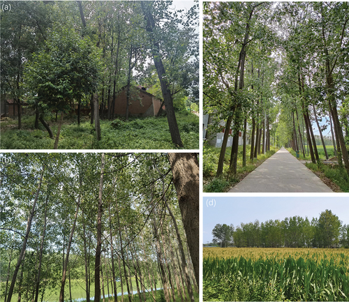
The majority of AGB or GSV modeling studies are located in mountainous regions because of the large proportion of forest coverage with relatively large patch sizes of forest lands (Duro, Franklin, and Dube 2012; Hirata et al. 2018; Lin et al. 2022). The fact that AGB or GSV accounted for a limited portion makes GSV estimation studies less attractive. The fragmentally distributed patches in plain regions, in particular, mixed-plot problem caused by striped distribution, make GSV estimation highly uncertain using traditional grid-based approaches (Bai et al. 2022). As an example, Figure 1 shows spatial distribution of poplar trees in “four-sides” with high heterogeneity of tree structure along the sides of houses (a), relative homogeneity of forest structure along the river (b), striped patterns along the road (c) and farmland (d). Considering the extensive distribution of poplar tree species but lack of proper approaches to estimate its GSV in plain regions, this research aims to explore potential solutions to quickly and accurately map GSV distribution. Specifically, this research attempts to identify a proper approach to estimate poplar GSV using airborne LIDAR data and to solve the poor prediction performance in the striped feature through a comparative analysis of grid-based and object-based modeling approaches. This research will be valuable for providing a solution to map GSV distribution of other tree species in plain regions, too.

Figure 1. Spatial patterns of poplar distributions in plain regions.

2. Study areas

Anhui Province is located in East China, extending across Yangtze River and Huai River valleys (Figure 2(a)). The terrain is diverse, including mountains, hills, and plains, and consists of five typical landform regions: Huai River plain region, Jianghuai hilly platform region, western Anhui hilly mountain region, riverside plain region, and southern Anhui hilly mountain region. There are two mountains – Dabie in southwestern and Baiji in southeastern in this province. Anhui province resides in the transitional area between a warm temperate zone and a subtropical zone. The north of the Huai River has a warm temperate semi-humid monsoon climate, and the south of the Huai River has a subtropical humid monsoon climate.

Figure 2. The study areas Lixin County and Yongqiao District in Anhui Province, China: (a) shows topography of Anhui Province by digital elevation model (DEM), (b) and (c) show spatial distributions of poplar species with sample plots in Yongqiao and Lixin, respectively.

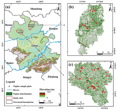
Poplar is one of the main afforestation tree species in Anhui Province. Since 2000, the implementation of projects including the Green For Grain (GFG) Program, the Yangtze River Shelter Forest Construction Project, the Snail Control and Schistosomiasis Prevention Forest Project, and the Fast-Growing and High-Yield Plantation Project has largely facilitated a rapid expansion of poplar plantations (Miao et al. 2018). The planted area reached 587,000 ha, accounting for 20% of the total forestry lands, and plays an important role in securing wood supply security and ecological security. In order to explore the poplar GSV, two typical plain regions – Lixin County in the southern part of the Huai River plain and Yongqiao District of Suzhou City in the northeastern part of the Huai River plain – were selected as case studies (Figure 2(b,c)). Poplar plantations in these study areas exhibited significant differences in spatial distribution patterns and stand structure characteristics. In Lixin County, the poplar forests with diverse stand structures were highly fragmented due to human intervention (Xi 2019; Zhu et al. 2022), while in Yongqiao District, large patches of the poplar forests were distributed along riverbanks and roadsides.

3. Materials and methods

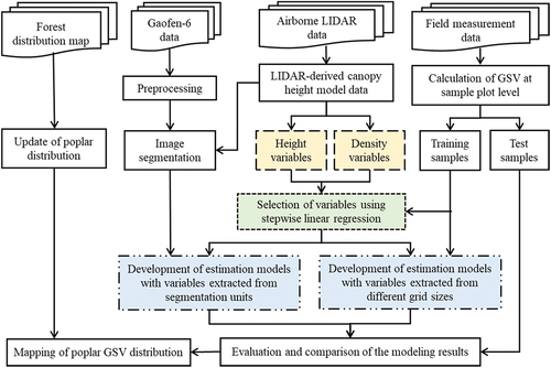
The framework for estimating poplar GSV consists of following steps (Figure 3): (1) data collection and preprocessing, including collection of poplar sample plot data and calculation of poplar GSV at sample plot level, collection and preprocessing of Gaofen-6 (GF-6) panchromatic and multispectral images and airborne LIDAR data; (2) update of poplar plantation distribution based on forest map and image segmentation based on the fused GF-6 multispectral images; (3) extraction of explanatory variables from LIDAR derived CHM at various statistical units, i.e. segments, and different grid sizes; (4) development of GSV estimation models using stepwise linear regression according to object-based and grid-based scenarios; (5) evaluation of modeling results and application of the developed models to the entire study areas.

Figure 3. Framework for developing poplar forest growing stock volume (GSV) estimation models based on airborne LIDAR and Gaofen-6 data.

3.1. Data preparation

The datasets used in this study include field measurements of sample plots, airborne LIDAR, GF-6 multispectral images, and a forest map of Anhui Province (Table 1). The qualities of these datasets were examined, especially for the geometric accuracy among these datasets.

Table 1. The datasets used in this study.

Datasets	Acquisition dates	Descriptions
Field measurements	June–September 2019	Sample plot size of 25.82 m by 25.82 m
Airborne LIDAR	June 2019	Point density of over 2 point/m^2
Gaofen-6 imagery	9 July 2019	Panchromatic image with a spatial resolution of 2.1 m and multispectral images of 4 bands with a spatial resolution of 8 m
Forest map	2019	Forestland “One Map” in vector format

3.1.1. Collection of field measurement data and calculation of growing stock volume at plot level

Field surveys in Lixin and Yongqiao were conducted between June and September 2019. Sample plots (25.82 m × 25.82 m) were established according to the spatial distributions and ages of poplar forests. For each plot, the precise geographical coordinates of the plot center and the four corners were recorded using Phantom P40 Unistrong Beidou No. 3 High Precision Positioning Board. Using advanced swan anti-jamming technology, the P40 instrument provides high precision positioning (horizontal position error within 0.5 m) (http://unistrong.com/Product/ProShow.aspx?proid=P40). All trees with a Diameter at Breast Height (DBH) greater than 5 cm within a plot were measured and recorded. The measured parameters include tree species, DBH, tree height, and crown width. Overlaying poplar sample plots on GF-6 multispectral image and airborne LIDAR data showed that some sample plots were shifted with high position errors. Thus, these sample plots were excluded from the field measurement dataset. A total of 43 plots in Lixin and 18 plots in Yongqiao were used in this research. The volume of an individual tree was calculated based on the measured DBH using the poplar volume allometric equation specific for Anhui Province (Anhui Forestry Bureau 2020), then GSV of a plot in m³/mu (1 mu = 666.7 m²) was obtained by summing volumes of all trees within the sample plot. The volume at plot level in m³/mu was converted into cubic meters per hectare (m³/ha). Table 2 summarizes DBH and GSV statistics for sample plots of both study areas.

Table 2. The DBH and GSV statistics of poplar sample plots.

Study areas	Number of sample plots	DBH (cm)			GSV (m^3/ha)
		Range	Mean	Standard deviation	Range	Mean	Standard deviation
Linxin	43	5.00–58.00	17.98	7.33	51.60–175.31	117.96	27.95
Yongqiao	18	5.20–61.80	16.95	8.06	19.45–183.65	118.45	53.02

3.1.2. Collection and preprocessing of airborne LIDAR data

Airborne LIDAR point cloud data of Lixin and Yongqiao were acquired by the RIEGL-VQ-1560i LIDAR scanning system in June 2019. The average point density was over 2 points/m². The data providers have already classified the LIDAR point clouds into ground and non-ground points. The Lidar360 software package was used to process the point cloud data. The ground points were used to generate a DTM, and the first return points were used to generate a DSM at a cell size of 1 m using Inverse Distance Weighting Interpolation method. The CHM was obtained by subtracting DTM from DSM. The abnormal cell values in CHM, including power lines, poles, and towers, as well as negative values or values greater than 50 m, were carefully examined against the airborne multispectral images, and refined by mean filtering.

3.1.3. GF-6 data collection and processing

GF-6 satellite imagery was acquired on 9 July 2019. This imagery consists of a panchromatic band with a spatial resolution of 2.1 m and four multispectral bands (blue, green, red, and near-infrared) with a spatial resolution of 8 m. Image preprocessing, including atmospheric calibration and ortho-rectification, was conducted. The Gram–Schmidt data fusion method (Karathanassi, Kolokousis, and Ioannidou 2007) was then used to fuse the panchromatic image with multispectral images to generate a new multispectral imagery with 2 m spatial resolution.

3.1.4. Update of spatial distribution of poplar plantations

To predict poplar GSV of the study areas, the spatial distribution of poplar plantations is needed. The forestland “One Map” of Anhui Province in 2019 in vector format was obtained from the Institute of East China Inventory and Planning, National Forestry and Grassland Administration. It was originally generated by visual interpretation of high spatial resolution satellite images. For each polygon in the map, attributes such as forest type and dominant tree species were attached. From this map, poplar plantations in Yongqiao were extracted and examined against the fused GF-6 multispectral imagery. Some poplar polygons with incorrect boundaries were manually modified. For Lixin County, poplar plantations were generated using a hierarchy-based classification algorithm based on fused images of ZY-3 panchromatic band and Sentinel-2 multispectral data (Zhao et al. 2022). The user’s and producer’s accuracies for poplar plantations were 97.44% and 90.60%, respectively.

3.1.5. Image segmentation

Image segmentation is the process of partitioning an image into homogeneous segments (or called objects); thus, the pixels within an object share similar characteristics, but the pixels from adjacent objects are significantly different. Of different image segmentation techniques, the Multiresolution Segmentation Algorithm (MSA) is one of the most widely used for the delineation of land cover or vegetation boundaries (Rahman and Saha 2008; Witharana and Civco 2014; Munyati 2018). In this study, the fused GF-6 multispectral images and airborne LIDAR CHM data were used as main data sources for image segmentation using MSA in eCognition software, while the updated poplar distribution map was used as a thematic layer. MSA requires a couple of parameters, including image band weights, scale, shape, and compactness values, to be pre-specified. In order to obtain as many segments completely covering field sample plots, the minimum object size was set at 26 m × 26 m. After iterative trial and error experimentation of various parameter combinations by visually examining the resulting segments against LIDAR CHM and GF-6 images, an optimal setting as scale parameter of 40, shape index of 0.6, smoothness weight of 0.7, compactness weight of 0.3, LIDAR CHM weight of 1.0, and GF-6 image weight of 0.5 was determined. Overlaying the sample plots on the resulting segments of the two study areas showed that 13 of the total 43 sample plots in Lixin did not completely fall into a single segment, while it was zero in Yongqiao. Thus, 30 sample plots in Lixin and 18 sample plots in Yongqiao, which were completely contained by a segment, were used in the object-based model development.

3.2. Extraction of variables from LIDAR CHM data and design of modeling scenarios

To extract explanatory variables from LIDAR data for GSV modeling, the statistical units were first determined. This process is established by MATLAB. Two types of statistical units were examined. One is the segments resulting from the segmentation of GF-6 multispectral images and LIDAR CHM. The segment sizes varied, depending upon the patch size of a homogenous forest stand; another is the grids with different square sizes. Generally, the poplars were planted with trees spaced about 2 m within the row and 4 − 6 m between the rows, and the average crown widths were 4 − 12 m (Dong et al. 2020; Xi 2019), especially for shelterbelt forests. Thus, the minimum grid size was set to be 10 m × 10 m, while the maximum was set to be 26 m × 26 m, which is close to the size of the field sample plot. Between the two are 15 m × 15 m and 20 m × 20 m.

Forest canopy-height-related variables, including height metrics (minimum, mean, maximum, and height percentiles; 10^th, 20^th, 30^th, 40^th, 50^th, 60^th, 70^th, 75^th, 80^th, 85^th, 90^th, 95^th, 98^th) and height variation variables (height standard deviation, kurtosis, skewness) within the predefined statistical units, were extracted from LIDAR CHM data. Stand complexity often impacts the relationships between canopy heights and GSV, and the canopy heights alone may not be sufficient to build an accurate GSV estimation model (Alonzo et al. 2018; Brede et al. 2019; Gao and Zhang 2021). Thus, for structurally complex stands, it is necessary to introduce new variables to enhance the prediction power. Therefore, CHM density was introduced into model development. To determine the CHM density, the vertical space between the maximum and the minimum heights within a statistical unit was divided into 10 equal-sized bins (layers), and the ratio of the number of cells falling into each bin to the total number of cells within a statistical unit represents the CHM density of each vertical layer. The equation of CHM density calculation can be expressed as

(1) ${\rho }_j=\hspace{0.17em}\frac{A_j}{A_{all}}$(1)

where ${\rho }_j$ represents CHM density at bin j, A_j is the number of CHM cells within bin j, A_all is the total number of cells within a statistical unit, and j equals 1 to 10, corresponding to the bin from the lowest to the highest layer. The vertical height space of bin j is defined by Equation (2)(2) $\left[\left(H_{\mathrm{m}\mathrm{i}\mathrm{n}}+\frac{H_{\mathrm{m}\mathrm{a}\mathrm{x}}-H_{\mathrm{m}\mathrm{i}\mathrm{n}}}{10}\left(j-1\right)\right),\left(H_{\mathrm{m}\mathrm{i}\mathrm{n}}+\frac{H_{\mathrm{m}\mathrm{a}\mathrm{x}}-H_{\mathrm{m}\mathrm{i}\mathrm{n}}}{10}\right)\right]$(2) :

(2) $\left[\left(H_{\mathrm{m}\mathrm{i}\mathrm{n}}+\frac{H_{\mathrm{m}\mathrm{a}\mathrm{x}}-H_{\mathrm{m}\mathrm{i}\mathrm{n}}}{10}\left(j-1\right)\right),\left(H_{\mathrm{m}\mathrm{i}\mathrm{n}}+\frac{H_{\mathrm{m}\mathrm{a}\mathrm{x}}-H_{\mathrm{m}\mathrm{i}\mathrm{n}}}{10}\right)\right]$(2)

where H_max and H_min are the maximum and minimum heights within a statistical unit. Thus, all these variables (canopy height metrics, stand structures, and density) were extracted at the units of segments and four grid sizes as input in GSV modeling.

After the variables were extracted from the CHM data, different scenarios were designed according to the variable types and the statistical units at which they were extracted. These scenarios have two objectives: (1) Investigating the role of density variables in GSV estimation models: All variables were extracted at a grid size of 26 m × 26 m, which is a similar size as the field sample plot (25.82 m × 25.82 m) commonly used in previous research (e.g. Feng et al. 2017; Jiang et al. 2020; Lin et al. 2022). Canopy-height-related variables alone and combinations of canopy height variables with density variables together as predictive variables were fitted sequentially to the models using the sample plots in the two study areas; (2) Examining the effect of the statistical units on model performances: Combinations of canopy height variables and density variables extracted at segment and different grid sizes (10 m × 10 m, 15 m × 15 m, 20 m × 20 m, 26 m × 26 m) were used as predictors to develop models in two study areas, respectively. A comparative analysis of results would show whether density variables can improve model accuracy, what grid size is optimal for variable extraction in developing GSV estimation models in two study areas, and the role of object-based modeling approach on prediction results compared with grid-based modeling results.

3.3. Variable selection and GSV modeling

One of the important steps in building a GSV estimation model is to identify key prediction variables. Different approaches such as stepwise regression, random forest, and lasso can be used to select key variables for GSV modeling (Lin et al. 2022). Based on our previous research using LIDAR data for modeling AGB or GSV and this exploration between GSV and LIDAR-derived metrics, linear relationship can be better expressed than nonlinear or machine learning algorithms (e.g. random forest) (Feng et al. 2017; Jiang et al. 2020; Lin et al. 2022); thus, this research used the stepwise linear regression method in SPSS for variable selection and poplar GSV modeling.

Linear regression assumes linear relationships between predictive variables and a response variable, specifically, LIDAR-CHM derived variables and poplar GSV here. It can be expressed as

(3) ${\mathrm{v}}_i={\mathrm{b}}_0+b_1{x}_{1i}+b_2{x}_{2i}+\dots +b_{\mathrm{p}}{x}_{\mathrm{p}i}+{\epsilon }_i$(3)

where v_i is poplar GSV of the sample plot i, b₀ is a constant, x₁, x₂, … , x_p are the selected variables from LIDAR CHM derived variables, b₁, b₂, … , b_p are the regression coefficients associated with predictive variables x₁, x₂, … , x_p, p is the number of predictive variables, and ɛ_i is the error term.

Stepwise regression has the ability to determine which variables should be kept in or eliminated from the final model according to the pre-specified criteria. Variable selection and model development with stepwise linear regression can be achieved by taking one of three approaches, i.e. forward selection, backward elimination, and bidirectional elimination. In this study, we applied a forward selection approach combined with the F-statistical test for variable selection, by setting the F test level of 0.1 and the significance level of 0.05 to determine whether a variable should be included or not. Forward selection starts with only the intercept and adds one potential variable at a time to test its significance. If a variable is statistically significant, it is included in the model; otherwise, it is excluded from the model. The process is repeated until the results are optimal (Gao et al. 2018; Jiang et al. 2020; Lin et al. 2022). Meanwhile, the Variance Inflation Factor (VIF) was used to examine the collinearity between the selected variables (Belsley, Kuh, and Roy 2005).

3.4. Evaluation and comparison of modeling results

The model fit was evaluated by the coefficient of determination (R²_fit) which was calculated based on the observed values and predicted values of the training samples (Lin et al. 2022). Once a model is developed based on the training samples, it is necessary to test its prediction performance or robustness using independent test samples. Common statistical measures used for evaluating model robustness include R², RMSE, and relative RMSE (RMSEr), which were calculated based on observed values and predicted values of the test samples (Puliti et al. 2018). Considering the limited field survey samples due to high cost and intensive labor during data collection, a K-fold cross-validation by means of MATLAB was used to test the effectiveness of the model (Puliti et al. 2018; Ehlers et al. 2022). With K-fold cross-validation, the entire sample dataset is randomly split into K-folds (usually K = 5 to 10 depending on the data size), among which K-1 (K minus 1) folds are used as training samples to fit the model, and the remaining one fold is used as test samples to validate the model. This process is repeated K times until each of K-fold serves as the test samples. Leave-one-out cross-validation is a special form of cross-validation. Supposedly, there are n samples in a dataset, then n-1 samples are used to build the model, leaving one sample to validate the model. It iterates n times till every sample is used once for testing (Jiang et al. 2021; Lin et al. 2022). This study conducted leave-one-out cross-validation and computed R², RMSE, and RMSEr for the models developed under different scenarios. In addition, the scatter plots between poplar GSV observation values and corresponding model-estimated GSV values were constructed for visual examination of model performances under different scenarios. The best models for each study area were selected to estimate poplar GSV over the corresponding study area.

In order to evaluate the differences between the object-based and grid-based modeling prediction results, a stratified random sampling approach with a total of 1000 samples used to locate each sample plot with plot size of 20 m × 20 m each in Lixin and Yongqiao, respectively. These samples were separated into three types: fully covered poplar, partially covered poplar, and non-poplar samples through examining the samples on the poplar distribution map with 2 m spatial resolution. The analysis was focused on the samples with fully covered and partially covered poplar within the plot size. The spatial join tool from ArcGIS was used to obtain the object-based prediction values corresponding to each sample plot. Scatter plots based on grid-based and object-based modeling results were then compared. Meanwhile, the total GSV and area of poplar plantations for both study areas were calculated from the prediction results, and comparative analyses of these results were examined by assigning the object-based GSV as reference data.

4. Results

4.1. Comparative analysis of variables in modeling growing stock volume

The results from model fitting with stepwise linear regression at grid size of 26 m × 26 m indicate that the relationships between poplar GSV and canopy height variables and density variables varied in two study areas (Table 3). When canopy height variables were used as explanatory variables in stepwise linear regression, H₈₅ in Lixin and H₇₀ in Yongqiao were selected. However, the R²_fit in Yongqiao with variable H₇₀ (R²_fit = 0.92) is much higher than that in Lixin with variable H₈₅ (R²_fit = 0.50). When canopy height variables and density variables were combined to fit the regression model in Lixin, R²_fit increased from 0.50 to 0.76, but no density variables were recruited into the regression model in Yongqiao, so R²_fit remained unchanged. Cross-validation of models also showed the same conclusions, indicating that density variables greatly improved the overall prediction accuracy. However, they have no effect on prediction accuracy in Yongqiao. This finding implies that the role of density in the GSV model varied, depending on the polar stand characteristics in each study area, specifically, Lixin has heterogeneous stand structure and tripped distribution, while Yongqiao has homogeneous stand structure with large patch sizes.

Table 3. Poplar GSV estimation models using LIDAR CHM-derived variables at a plot size of 26 m × 26 m.

Study areas	Predictive variables	GSV estimation model fitting		Model validation
		Linear models	R^2fit	R^2	RMSE (m^3/ha)	RMSEr (%)
Lixin	Height	−32.71 + 7.74H85	0.50	0.46	20.23	17.15
	Height & Density	−26.28 + 13.31H10 + 6.07H85 − 2.86D4 + 3.12D7 − 5.62D9 + 4.18D10	0.76	0.71	14.94	12.67
Yongqiao	Height	−24.71 + 8.46H70	0.92	0.89	16.59	14.50
	Height & Density	Same as the model with height variables		Same as the model with height variables

H_i is the ith height percentile; D_j is density at the jth layer.

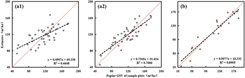
The relationships between the predicted poplar GSV values from the developed models and the observed GSV of sample plots (Figure 4) indicate overestimation for the low GSV (less than 80 m³/ha) and underestimation for the high GSV (greater than 150 m³/ha) in both study areas. The model in Yongqiao performed better than in Lixin from the point distributions along the 1:1 line. For Lixin, the overestimation and underestimation were much improved after incorporating density variables into CHM metrics (Figure 4(a2)), implying the importance of taking the complex forest structures into account when developing GSV estimation model.

Figure 4. Relationships between the predicted poplar growing stock volume using developed models and observed values of sample plots, including the scatter plots in Lixin which the models were developed using canopy height variables (a1) and a combination of canopy height variables and density variables (a2); the scatter plot in Yongqiao which the model was developed using canopy height variables only (b).

4.2. Comparative analysis of modeling results based on different modeling units

The developed models based on the LIDAR derived variables at different statistical units and their validation results (Table 4) indicate that with the grid-based method, as the grid size increases, the estimation accuracy increases till to a grid size of 20 m × 20 m, then decreases as the grid size expands to 26 m × 26 m for both study areas. Table 4 shows that a grid size of 20 m × 20 m as a statistical unit achieved the best estimation accuracy. However, the model in Lixin contains multiple predictive variables, including height variables (H₈₆ and H₁₀) and density variables (D₉ and D₇), while the model in Yongqiao is much simpler with only one predictive variable, H₇₀. One interesting thing about grid-based models in Lixin is that for the plot size became 20 m × 20 m or 26 m × 26 m, more variables were included, in particular, inclusion of density variables considerably improved the R² values. Checking the VIF values found that the values were between 1.23 and 3.8 for 20 m × 20 m, and between 1.68 and 6.51 for 26 m × 26 m, implying these variables were needed and had less collinearity problem (Belsley, Kuh, and Roy 2005). In addition, when grid sizes were relatively small (10 m × 10 m and 15 m × 15 m), the models in Lixin were simple with only one height variable (H₉₀), but the estimation accuracies were relatively poor with low R² (0.48 and 0.51) and high RMSE values (19.88 m³/ha and 18.90 m³/ha). In contrast, all models in Yongqiao contained only one canopy height variable for different grid sizes, but the variables, i.e. height percentiles, varied from H₇₀ to H₈₅. Based on the bias results in Table 4, the GSV estimates in Lixin County had high potential to be overestimated, while in Yongqiao, they had the potential to be underestimated. The bias results also confirmed that a plot size of 20 m × 20 m had the best modeling performance.

Table 4. Summary of GSV estimation accuracy assessment results based on different scenarios.

Study areas	Statistical unit (m^2)		GSV estimation models	R^2fit	Model validation
					R^2	RMSE (m^3/ha)	RMSEr (%)	Bias (m^3/ha)
Lixin	Grid-based	10 × 10	−2.63 + 6.245H90	0.52	0.48	19.88	16.85	4.29
		15 × 15	−17.37 + 6.82H90	0.56	0.53	18.90	16.02	3.02
		20 × 20	−23.35+7.34H85	0.58	0.54	18.68	15.84	3.16
		20 × 20	−77.35+10.78H10+8.43H85 +2.24D7$-$3.33D9	0.78	0.74	14.02	11.89	1.62
		26 × 26	−26.28+13.31H10+ 6.07H85+4.18D10 $-$5.62D9$-$2.86D4+ 3.12D7	0.76	0.71	14.94	12.67	14.75
	Object-based		−39.87 + 7.53H90	0.61	0.56	13.82	11.66	4.88
Yongqiao	Grid-based	10 × 10	−18.92 + 7.40H80	0.88	0.86	18.73	16.37	−2.46
		15 × 15	−24.46 + 7.75H85	0.90	0.88	16.79	14.67	−2.48
		20 × 20	−18.15 + 8.02H70	0.91	0.90	15.99	13.97	−0.65
		26 × 26	−24.72 + 8.46H70	0.92	0.89	16.59	14.50	−4.04
	Object-based		−24.64 + 9.17H60	0.91	0.90	15.84	13.85	0.01

H_i is the ith percentile of canopy height; D_j is density at the jth layer.

Considering the results from grid-based and object-based models (Table 4), the object-based variable extraction method (segment as a statistical unit) resulted in simple regression models. The object-based model in Lixin contains only one canopy height variable (H₉₀) but produced similar modeling accuracy to the complex model associated with a grid size of 20 m × 20 m did in terms of RMSE and RMSEr. The object-based model in Yongqiao slightly improved estimation accuracy compared to grid-based models, and canopy height H₆₀ was selected as the only predictive variable. The selected variables between object-based and grid-based modeling approaches may imply the different impacts of forest stand structures on GSV modeling performance.

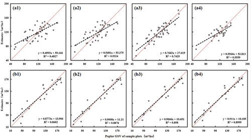
The scatter plots between the observed poplar GSV of sample plots and the GSV estimates from the developed models at different scenarios (Figure 5) show that with smaller grid sizes (e.g. 10 m × 10 m and 15 m × 15 m) the points are scattered far away from the 1:1 line, especially for Lixin (Figure 5(a1,a2)), indicating the high discrepancy between estimates and observed GSV values and poor model performance. When the grid size is increased to 20 m × 20 m (Figure 5(a3)), the points are much closer to the 1:1 line, implying better prediction performance. Compared to the grid-based approach, object-based models reduced overestimation and underestimation situations (Figure 5(a4,b4)). It is worth noting that in Lixin, the number of sample plots (n = 30) used for model fitting in the scenario of an object-based approach is less than that of the original sample dataset (n = 43) because there are 13 sample plots intersecting with more than one segment. This can be clearly seen in Figure 5(a4), where most of the low GSV and high GSV sample plots were missing.

Figure 5. Relationships between observed poplar GSV of sample plots and estimated GSV based on different scenarios: (a1) to (a4) represent the statistical units at which the variables were extracted 10 m × 10 m, 15 m × 15 m, 20 m × 20 m, and segment, respectively in Lixin, (b1) to (b4) represent the same statistical units in Yongqiao.

4.3. Poplar GSV estimation over the entire areas

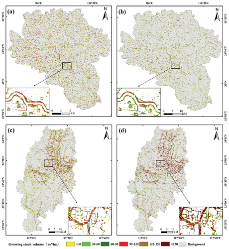
The best grid-based models with a grid size of 20 m × 20 m and object-based models in Lixin and Yongqiao were selected and used to estimate the GSV of the entire study areas, generating the GSV spatial distribution maps (Figure 6). It indicates that the majority of GSV values in Lixin are lower than 60 m³/ha and stochastically scattered among other land use types, especially in farmlands. High GSV values (> 150 m³/ha) are much more widely distributed (Figure 6(b)), primarily along rivers or in plantation forests with more regular shapes and larger extents. In Yongqiao, poplar forests are more concentrated along rivers and wide roads (Figure 6(d)). The aggregated poplar patches often cover large areas, and high GSV values (> 150 m³/ha) account for a large portion of them.

Figure 6. The growing stock volume estimates at segments (a) and (c) and grid sizes of 20 m × 20 m (b) and (d) in Lixin and Yongqiao ((a) and (b) for Lixin; (c) and (d) for Yongqiao).

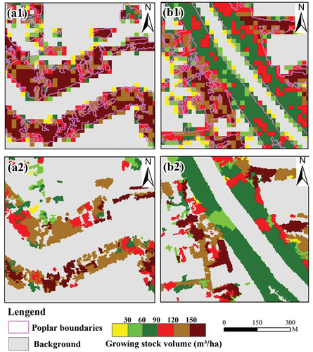
The comparison of predicted results from grid-based and object-based approaches (Figure 7) indicated that the objected-based approach is more suitable for strip-distributed poplar plantations in both study areas. Due to mixed plot problems on the edges of poplar patches (Figure 7(a1,b1)), the conventional grid-based approach produced GSV distributions with larger extents than the true poplar extents, and GSV at those superfluous cells is frequently lower than at the center cells. In addition, since the basic unit of the grid-based approach is a grid, the resulting GSV distributions are not smooth with a lot of salt-and-pepper cells. The object-based method (Figure 7(a2,b2)) generates GSV distributions with distinct object boundaries, which is more similar to the reality of poplar distributions. This comparison indicates the advantage of using the object-based approach over using the grid-based approach in mapping GSV distributions, especially for poplar plantations with striped patterns.

Figure 7. Poplar growing stock volume estimates of typical poplar strip forests from grid-based and object-based approaches: (a1) and (a2) represent grid-based estimates based on grid size of 20 m × 20 m and object-based estimates in Lixin, (b1) and (b2) represent grid-based object-based estimates in Yongqiao.

Comparison of GSV estimates (Table 5) indicates that the grid-based approach predicts a much higher GSV amount in Lixin County than the object-based approach. The overestimation rate can reach 55.46% [(GSV_grid−GSV_object)/GSV_object × 100], and in contrast, the overestimation rate in Yongqiao District is only 13.6% when the object-based modeling GSV estimate is used as reference data. Because of the strip distribution of poplar plantations in plain regions, the areal calculation based on grid size of 20 m × 20 m is also much higher than the object-based poplar area, as shown in Table 5 that the overestimation rate in Lixin can be as high as 82.62%. This high overestimation in area and GSV amount using the grid-based approach implies the high impact of patch size and shape on the predicting results. This situation indicates the necessity of conducting the calibration of modeling results to reduce the high uncertainty caused by overestimated area in the grid-based modeling approach.

Table 5. A comparison of estimated total GSV amounts in both study areas.

Study area	Grid-based calculation		Object-based calculation		GSV rate (%)	Area rate (%)
	GSV (×10^6 m^3)	Area (ha)	GSV (×10^6 m^3)	Area (ha)
Lixin	1.9631	30952.04	1.2628	16949.01	55.46	82.62
Yongqiao	2.0076	25504.28	1.7672	20549.35	13.60	24.11

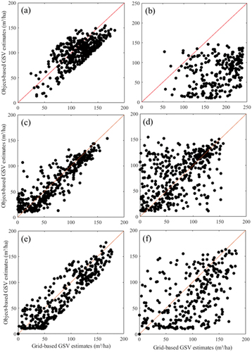
The scatter plots between the grid-based GSV estimates and the object-based GSV estimates show that both modeling approaches have very strong relationships for the fully covered poplar plots, but not for partially covered poplar plots because the estimates are mostly away from the 1:1 line (Figure 8). A comparative analysis of the GSV modeling results with and without the use of density variables indicates that incorporation of CHM metrics and density variables indeed improved modeling performance for the fully-covered poplar areas (see Figure 8(a,c)), but not for the partially covered poplar areas (see Figure 8(b,d)). This could be the major reason resulting in a high overestimation of the overall GSV amount in Lixin county (see Table 5) if the modeling sampling is mainly from the fully covered poplar plots. Instead, the grid-based model without use of density variables provides better prediction results for the partially covered poplar plots than the model with incorporated density variables, implying that an overall better modeling performance cannot guarantee a better prediction result.

Figure 8. A comparison of scatter plots based on the GSV estimates from grid-based (20 m × 20 m) and object-based modeling approaches in Lixin ((a), (b) are based on the combination of CHM metrics and density variables; (c), (d) are based on CHM metrics only; (a), (c) include fully covered poplar plots while b, d include partially covered poplar plots) and Yongqiao ((e) means fully covered poplar plots, (f) means partially covered poplar plots).

5. Discussion

5.1. Impacts of forest stand structure on GSV modeling performance

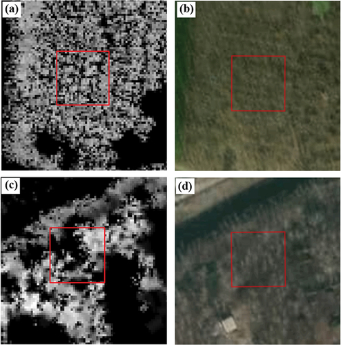
Forest stand structure has been regarded as an important factor influencing the selection of the potential variables and modeling approaches (Lu et al. 2016; Hernández-Stefanoni et al. 2018; Zhou et al. 2019; Thi Kim Cuc and Hien 2021). Previous research in tropical and subtropical regions has indicated that different tree species compositions and different tree densities affect the stand structure complexity, thus affecting the selection of spectral and textural variables when using optical sensor data or SAR (Lu, Batistella, and Moran 2005; Zhao et al. 2016; Ehlers et al. 2022; Tamiminia et al. 2022; González-Ferreiro et al. 2013). Even using CHM-derived variables from LIDAR data, different forest stand structures, such as Chinese fir and Masson pine, require the selection of different variables for AGB or GSV estimation modeling (Jiang et al. 2020; Lin et al. 2022). This research further confirms that in plain regions, differences in poplar stand structures and heterogeneity conditions in Lixin and Yongqiao affect the selection of variables and modeling performance. Figure 9 exemplifies two poplar sample plots with the distinguishing stand characteristics located in Yongqiao (Figure 9(a,b)) and Lixin (Figure 9(c,d)) based on LIDAR CHM and high spatial resolution images. They clearly show that poplar trees are not evenly distributed within the sample plot in Lixin. There exist large gaps within poplar patches (dark region on the CHM map), causing a high variation in canopy height within the sample plot. Actually, in striped poplar forests, it is hard to find large patches, which meet requirements for a standard sample plot in size and stand characteristics. In contrast, the sample plot in Yongqiao completely falls into a poplar plantation, where similar-height trees with a dense canopy and fine texture are regularly distributed. Due to differences in poplar stand characteristics in Lixin and Yongqiao, the variables used in modeling vary. In Yongqiao, where poplar plantations are homogenous, canopy height variables alone can sufficiently characterize GSV, while in Lixin, where poplar plantations have diverse vertical structures, a combination of height variables and density variables is necessary to obtain high accuracy in GSV estimates.

Figure 9. Two poplar sample plots from Yongqiao ((a) and (b)) and Lixin ((c) and (d)) showing the differences in poplar stand structures from LIDAR CHM ((a) and (c)) and high spatial resolution images ((b) and (d)).

Many studies have proven the advantages of using canopy height variables over optical or SAR data in AGB or GSV estimation (Feng et al. 2017; Alonzo et al. 2018; Li et al. 2019). In addition to the canopy height variables, the LIDAR point density variables are valuable for improving GSV modeling, but have not been fully examined yet. The density variables can be extracted from LIDAR point cloud data or CHM. If point cloud data are available, the density variables may be more accurately extracted than from CHM, but may take more time in data processing. In our research, we only have CHM data and the CHM-derived density variable proved valuable through combining them with height variables into regression models in improving modeling performance. The results showed that CHM density variables can improve overall modeling performance in Lixin, where the polar plantations have complex vertical structures, but had no effects on GSV models in Yongqiao, further confirming the important role of the density variables in improving the GSV estimation accuracy in forest areas with high vertical heterogeneity. Similar conclusion was also obtained by incorporating density variables and height variables from LIDAR (Duan et al. 2015) that R² value of 0.81 was obtained when estimating AGB in subtropical forests in Dinghushan, Guangdong province, China. Our research confirms the impacts of complex stand structure on modeling performance and the requirement of using density variable in this situation. However, our research has another interesting finding that incorporation of density variables into height variables mainly improved the prediction results for the fully covered poplar areas, but may not be useful for the partially covered poplar areas, as shown in Table 3 and Figure 8(b) that the prediction may be highly overestimated. This situation implies that caution should be taken for the use of density variables. More research is needed to decide whether or not to use the density variables for GSV modeling, especially for the plain regions with strip distribution of tree species.

5.2. Impacts of object-based and grid-based approaches on poplar GSV estimation

Remote sensing-based GSV mapping is generally conducted on uniform grids, a similar size as the sample plot (e.g. 20 m × 20 m). This is suitable for continuously distributed large forest extents, where the edges of forest types or species are not a major problem. However, in plain regions where many plantations exist in narrow strips as shown in Figure 1, their GSV is often estimated by directly using the models developed from the sample plots located in large forest areas (Mishra and Crews 2014; Campbell et al. 2021). For example, Bai et al. (2022) extracted canopy height variables from airborne LIDAR and spectral variables from multispectral images in Zhuhai New District and developed models based on the samples mainly located in forest parks. Those models were directly applied to striped trees on roadsides for biomass estimation, resulting in overestimation due to the boundary errors caused by mixed land cover problems on the forest edges. In this study, a large portion of poplar forests is distributed as strips in Lixin. When GSV estimation was performed by a conventional grid-based approach with a grid size of 20 m × 20 m, as shown in Figure 7, the plots crossing the poplar forest edges often contained non-poplar or forest types, such as roads and/or crops. The variables derived from LIDAR CHM for those plots actually represent the averages over the whole plot, not for poplar plantation alone, leading to inaccuracy of the extracted variables and consequently to inaccurate GSV estimates as shown in Figure 8.

The GSV estimation performed on a segment basis allows the GSV estimates to be on structurally homogeneous units of forests (Rahman and Saha 2008; Alonzo et al. 2018; Witharana and Civco 2014), reducing the variability within forest stands. In this study, a multiresolution segmentation approach was applied to the GF-6 multispectral image and LIDAR CHM with polar forest distribution as thematic map, and produced homogenous poplar patches. The object-based method avoids extracting variables from the forests with heterogeneous stand structures. Studies showed that the object-based approach is suitable not only in plain areas but also in mountainous areas where forests have complex species compositions and irregular shapes (Andersen et al. 2012; Silveira et al. 2018). Thus, the object-based approach has more universality and generalization. This research further confirmed the advantages of using the object-based modeling approach over the grid-based ones in poplar GSV estimation in plain regions, as shown in Figure 8.

Since the sample plots collected in this study were established according to the forest distribution without taking the patch size into account, some plots in Lixin were intersected with more than one segment. In this case, the plots had poor representativeness (as illustrated in Figure 9(c,d)) and cannot be used in model development, resulting in a smaller number of useful sample plots. Therefore, the object-based approach requires a sampling design of survey plots according to segmentation products, ensuring a plot is completely located in a segment. This research indicates that a good-fitting grid-based modeling performance cannot guarantee a good prediction performance. The major reason is that the modeling samples are from the representative forest sites that cannot reflect the mixed regions of forest and other land covers. This mixed land cover problem is especially serious in the plain regions, as shown in this study, that poplar GSV could be considerably overestimated using a grid-based approach compared with the object-based modeling approach (Table 5). Therefore, more research should be focused on reducing the impacts of the mixed plots (mixed poplar and other lands in a grid) on the prediction results.

5.3. Impacts of different grid sizes of variable extraction on poplar GSV modeling performance

A sufficient number of sample plots with good representativeness are essential for GSV modeling (Lu et al. 2016; Klinger et al. 2018). A plot must represent the entire forest stand in species composition, structure, and age, which means the necessity to select a suitable plot size. With the grid-based approach, sample plot sizes have a significant effect on GSV estimation accuracy (Frazer et al. 2011; Navarro-Cerrillo et al. 2017). Stereńczak et al. (2018) found that as sample plot size increased from 100 m² to 500 m² (100, 200, 300, 400, and 500 m²), the estimation accuracy of the regression models for AGB of dominant pine forests in Poland increased. A similar conclusion was drawn by Ju et al. (2022) who explored the correlation between the stand density and stand stock volume. This implies that a sample plot size reflects its representation of a forest stand structure. Another study conducted by Navarro-Cerrillo et al. (2017) found that when sample plot size increased from a radius of 7 m to 15 m, the AGB estimation accuracy of pine plantations in southern Spain based on airborne LIDAR significantly improved. However, when sample plot size was continuously expanded to a radius of 30 m, estimation accuracy decreased. Thus, the optimal sample plot size depends on the forest stand characteristics. Our study indicates that the optimal sample plot size for poplar forest in Lixin and Yongqiao is 20 m × 20 m. The larger the sample plot size, the more complex the stand structure within the sample plot, the more mixed land covers are contained within the entire study area (Zhou et al. 2019; Hosseini et al. 2021). A large plot size also means the need for more time and work load for field measurements.

The representativeness of the sample plots further magnifies or reduces the effect of position errors (Hernández-Stefanoni et al. 2018; Jurjević 2020). For example, the heterogeneity of stand structures within and near poplar sample plots in Lixin was obvious; thus, even a small shift in plot boundaries resulted in significant changes in variables such as height percentiles. On the contrary, similar stand characteristics are still maintained within the buffer zone of several tens of meters near the sample site in Yongqiao, and small positional errors of plots have limited impact on CHM-derived variables, and the correlation between height percentiles and GSV remains high, although the sample plot shape or size has changed to some degree. In addition, many poplar plantations are distributed in strips, and distances from the boundaries of a sample plot toward the edge of a poplar patch are often as short as less than 10 m. In this situation, errors due to mismatch between sample plots and LIDAR data have considerable impacts on the extracted variables and eventually affect the GSV prediction.

6. Conclusions

This study examined poplar GSV estimation in two plain areas in Anhui Province based on airborne LIDAR data through comparative analysis of modeling results using grid-based and object-based approaches. The key conclusions can be obtained as follows:

1. Poplar distribution patterns and forest stand characteristics affect the selection of predictive variables, modeling performance, and prediction results. The incorporation of density variables into modeling improved GSV estimation performance significantly in Lixin, where R² increased from 0.46 to 0.76, and the RMSEr decreased from 17.15% to 12.67% owing to the complexity of poplar stand structures; however, no density variable was required in GSV modeling in Yongqiao because of the relatively simple stand structures;

2. The object-based approach provided slightly better estimation accuracy in both Lixin and Yongqiao in terms of RMSE and RMSEr. The advantage of using an object-based modeling approach is the ability to solve the mixed plot problems, which is especially important in Lixin County where poplar forest is distributed in strips;

3. Selection of the proper grid size to extract variables from airborne LIDAR data influences GSV modeling performance. This research indicates that a grid size of 20 m × 20 m is best for poplar GSV modeling in both plain regions, but the grid-based modeling approach can produce high uncertainty in the prediction results due to the mixed plot problem.

Disclosure statement

No potential conflict of interest was reported by the author(s).

Data availability statement

Due to confidentiality agreements, supporting data can only be made available to bona fide researchers subject to a nondisclosure agreement. Details of the data and how to request access are available from Professor Dengsheng Lu at Fujian Normal University.

Additional information

Funding

This work was supported by the National Natural Science Foundation of China [grant number 32171787] and National Key R&D Program of China [grant number 2021YFD2200400102].

Notes on contributors

Ruoqi Wang

Ruoqi Wang is currently pursuing PhD degree at Fujian Normal University. Her research interests are remote sensing technologies and applications and forest volume/biomass modeling.

Guiying Li

Guiying Li received her PhD degree from Indiana State University and is an associate professor at Fujian Normal University. Her research interests are remote sensing, GIS, land use/cover change, and forestry.

Yagang Lu

Yagang Lu is a senior engineer at the Institute of East China Inventory and Planning, National Forestry and Grassland Administration. His research interests are forest inventory and remote sensing applications.

Dengsheng Lu

Dengsheng Lu is currently a professor at School of Geographical Sciences, Fujian Normal University, Fuzhou, China. He graduated from Indiana State University in 2001, majoring in Physical Geography with a specialty in Remote Sensing and GIS. He had worked at Indiana University at Bloomington (2001–2006; 2008–2012), Auburn University (2007–2008), and Michigan State University (2012–2018). His research interests include remote sensing technologies and applications in tropical and subtropical forest ecosystems, in particular, in land use/cover change and forest biomass/volume estimation. In recent years, his research funds are mainly from the National Key R&D Program of China and NSFC. He has published 150+ articles with Google Scholar citations of 24800 (early January 2023). Dr Lu was the “Most Cited Chinese Researchers” for the years 2019–2021. In the World’s Top 2% Scientists, Dr Lu was also within the “Career Long Impact” in 2020–2022 and “Single Year Impact” in 2019–2021. He is an editorial board member in the journals such as International Journal of Digital Earth, Geo-spatial Information Science, International Journal of Image and Data Fusion, Remote Sensing, and Frontiers in Remote Sensing.

References

- Alonzo, M., H. E. Andersen, D. Morton, and B. Cook. 2018. “Quantifying Boreal Forest Structure and Composition Using UAV Structure from Motion.” Forests 9 (3): 119. doi:10.3390/f9030119.
- Andersen, H. E., J. Strunk, H. Temesgen, D. Atwood, and K. Winterberger. 2012. “Using Multilevel Remote Sensing and Ground Data to Estimate Forest Biomass Resources in Remote Regions: A Case Study in the Boreal Forests of Interior Alaska.” Canadian Journal of Remote Sensing 37 (6): 596–611. doi:10.5589/m12-003.
- Anhui Forestry Bureau. 2020. “Poplar Tree Volume Tables, Anhui Provincial Standard, # DB34/T 3620-2020”.
- Astola, H., T. Häme, L. Sirro, M. Molinier, and J. Kilpi. 2019. “Comparison of Sentinel-2 and Landsat 8 Imagery for Forest Variable Prediction in Boreal Region.” Remote Sensing of Environment 223: 257–273. doi:10.1016/j.rse.2019.01.019.
- Baghdadi, N., G. Le Maire, J. Bailly, K. Ose, Y. Nouvellon, M. Zribi, C. Lemos, and R. Hakamada. 2015. “Evaluation of ALOS/PALSAR L-Band Data for the Estimation of Eucalyptus Plantations Aboveground Biomass in Brazil.” IEEE Journal of Selected Topics in Applied Earth Observations and Remote Sensing 8 (8): 3802–3811. doi:10.1109/JSTARS.2014.2353661.
- Bai, L., Q. Cheng, Y. Shu, and S. Zhang. 2022. “Estimating the Aboveground Biomass of Urban Trees by Combining Optical and Lidar Data: A Case Study of Hengqin, Zhuhai, China.” Photogrammetric Engineering & Remote Sensing 88 (2): 121–128. doi:10.14358/PERS.21-00045R2.
- Belsley, D. A., E. Kuh, and E. W. Roy. 2005. Regression Diagnostics: Identifying Influential Data and Sources of Collinearity. Hoboken: John Wiley & Sons.
- Blaschke, T. 2010. “Object Based Image Analysis for Remote Sensing.” Isprs Journal of Photogrammetry and Remote Sensing 65 (1): 2–16. doi:10.1016/j.isprsjprs.2009.06.004.
- Brede, B., K. Calders, A. Lau, P. Raumonen, H. M. Bartholomeus, M. Herold, and L. Kooistra. 2019. “Non-Destructive Tree Volume Estimation Through Quantitative Structure Modelling: Comparing UAV Laser Scanning with Terrestrial Lidar.” Remote Sensing of Environment 233: 111355. doi:10.1016/j.rse.2019.111355.
- Campbell, M. J., P. E. Dennison, K. L. Kerr, C. B. Simon, and W. R. L. Anderegg. 2021. “Scaled Biomass Estimation in Woodland Ecosystems: Testing the Individual and Combined Capacities of Satellite Multispectral and Lidar Data.” Remote Sensing of Environment 262 (9): 112511. doi:10.1016/j.rse.2021.112511.
- Cao, L., H. Liu, X. Fu, Z. Zhang, X. Shen, and H. Ruan. 2019. “Comparison of UAV Lidar and Digital Aerial Photogrammetry Point Clouds for Estimating Forest Structural Attributes in Subtropical Planted Forests.” Forests 10 (2): 145. doi:10.3390/f10020145.
- Chen, L., C. Ren, G. Bao, B. Zhang, Z. Wang, M. Liu, W. Man, and J. Liu. 2022. “Improved Object-Based Estimation of Forest Aboveground Biomass by Integrating Lidar Data from GEDI and ICESat-2 with Multi-Sensor Images in a Heterogeneous Mountainous Region.” Remote Sensing 14 (12): 2743. doi:10.3390/rs14122743.
- Chrysafis, I., G. Mallinis, M. Tsakiri, and P. Patias. 2019. “Evaluation of Single-Date and Multi-Seasonal Spatial and Spectral Information of Sentinel-2 Imagery to Assess Growing Stock Volume of a Mediterranean Forest.” International Journal of Applied Earth Observation and Geoinformation 77: 1–14. doi:10.1016/j.jag.2018.12.004.
- Dong, L., F. R. A. Widagdo, L. Xie, and F. Li. 2020. “Biomass and Volume Modeling Along with Carbon Concentration Variations of Short-Rotation Poplar Plantations.” Forests 11 (7): 780. doi:10.3390/f11070780.
- Dronova, I. 2015. “Object-Based Image Analysis in Wetland Research: A Review.” Remote Sensing 7 (5): 6380–6413. doi:10.3390/rs70506380.
- Duan, Z., D. Zhao, Y. Zeng, Y. Zhao, B. Wu, and J. Zhu. 2015. “Estimation of the Forest Aboveground Biomass at Regional Scale on Remote Sensing.” Geomatics and Information Science of Wuhan University 40 (10): 1400–1408. doi:10.13203/j.whugis20140709.
- Duro, D. C., S. E. Franklin, and M. G. Dube. 2012. “A Comparison of Pixel-Based and Object-Based Image Analysis with Selected Machine Learning Algorithms for the Classification of Agricultural Landscapes Using SPOT-5 HRG Imagery.” Remote Sensing of Environment 118: 259–272. doi:10.1016/j.rse.2011.11.020.
- Ehlers, D., C. Wang, J. Coulston, Y. Zhang, T. Pavelsky, E. Frankenberg, C. Woodcock, and C. Song. 2022. “Mapping Forest Aboveground Biomass Using Multisource Remotely Sensed Data.” Remote Sensing 14 (5): 1115. doi:10.3390/rs14051115.
- Feng, Y., D. Lu, Q. Chen, M. Keller, E. Moran, M. N. dos-Santos, E. L. Bolfe, and M. Batistella. 2017. “Examining Effective Use of Data Sources and Modeling Algorithms for Improving Biomass Estimation in a Moist Tropical Forest of the Brazilian Amazon.” International Journal of Digital Earth 10 (10): 996–1016. doi:10.1080/17538947.2017.1301581.
- Frazer, G. W., S. Magnussen, M. A. Wulder, and K. Niemann. 2011. “Simulated Impact of Sample Plot Size and Co-Registration Error on the Accuracy and Uncertainty of LiDar-Derived Estimates of Forest Stand Biomass.” Remote Sensing of Environment 115 (2): 636–649. doi:10.1016/j.rse.2010.10.008.
- Gao, L., and X. Zhang. 2021. “Above-Ground Biomass Estimation of Plantation with Complex Forest Stand Structure Using Multiple Features from Airborne Laser Scanning Point Cloud Data.” Forests 12 (12): 1713. doi:10.3390/f12121713.
- Gao, Y., D. Lu, G. Li, G. Wang, Q. Chen, L. Liu, and D. Li. 2018. “Comparative Analysis of Modeling Algorithms for Forest Aboveground Biomass Estimation in a Subtropical Region.” Remote Sensing 10 (4): 627. doi:10.3390/rs10040627.
- Georganos, S., T. Grippa, S. Vanhuysse, M. Lennert, M. Shimoni, S. Kalogirou, and E. Wolff. 2018. “Less is More: Optimizing Classification Performance Through Feature Selection in a Very-High-Resolution Remote Sensing Object-Based Urban Application.” GIScience & Remote Sensing 55 (2): 221–242. doi:10.1080/15481603.2017.1408892.
- González-Ferreiro, E., U. Diéguez-Aranda, L. Barreiro-Fernández, S. Buján, M. Barbosa, J. Suárez, and D. Miranda. 2013. “A Mixed Pixel- and Region-Based Approach for Using Airborne Laser Scanning Data for Individual Tree Crown Delineation in Pinus Radiata D. Don Plantations.” International Journal of Remote Sensing 34 (21): 7671–7690. doi:10.1080/01431161.2013.823523.
- Guo, Q., Y. Su, T. Hu, H. Guan, S. Jin, J. Zhang, X. Zhao, et al. 2021. “Lidar Boosts 3D Ecological Observations and Modeling: A Review and Perspective.” IEEE Geoscience and Remote Sensing Magazine 9 (1): 232–257. doi:10.1109/MGRS.2020.3032713.
- Hernández-Stefanoni, J., G. Reyes-Palomeque, M. Castillo-Santiago, S. George-Chacón, A. Huechacona-Ruiz, F. Tun-Dzul, D. Rondon-Rivera, and J. Manuel Dupuy. 2018. “Effects of Sample Plot Size and GPS Location Errors on Aboveground Biomass Estimates from Lidar in Tropical Dry Forests.” Remote Sensing 10 (10): 1586. doi:10.3390/rs10101586.
- Hirata, Y., N. Furuya, H. Saito, C. Pak, C. Leng, H. Sokh, V. Ma, T. Kajisa, T. Ota, and N. Mizoue. 2018. “Object-Based Mapping of Aboveground Biomass in Tropical Forests Using LiDar and Very-High-Spatial-Resolution Satellite Data.” Remote Sensing 10 (3): 438. doi:10.3390/rs10030438.
- Hosseini, Z., H. Latifi, H. Naghavi, S. Bakhtiarvand Bakhtiari, and F. Ewald Fassnacht. 2021. “Influence of Plot and Sample Sizes on Aboveground Biomass Estimations in Plantation Forests Using Very High Resolution Stereo Satellite Imagery.” Forestry: An International Journal of Forest Research 94 (2): 278–291. doi:10.1093/forestry/cpaa028.
- Hyde, P., R. Dubayah, W. Walker, J. B. Blair, M. Hofton, and C. Hunsaker. 2006. “Mapping Forest Structure for Wildlife Habitat Analysis Using Multi-Sensor (Lidar, SAR/Insar, ETM+, Quickbird) Synergy.” Remote Sensing of Environment 102 (1–2): 63–73. doi:10.1016/j.rse.2006.01.021.
- Jiang, F., M. Kutia, K. Ma, S. Chen, J. Long, and H. Sun. 2021. “Estimating the Aboveground Biomass of Coniferous Forest in Northeast China Using Spectral Variables, Land Surface Temperature and Soil Moisture.” The Science of the Total Environment 785: 147335. doi:10.1016/j.scitotenv.2021.147335.
- Jiang, X., G. Li, D. Lu, E. Chen, and X. Wei. 2020. “Stratification-Based Forest Aboveground Biomass Estimation in a Subtropical Region Using Airborne Lidar Data.” Remote Sensing 12 (7): 1101. doi:10.3390/rs12071101.
- Ju, Y., Y. Ji, J. Huang, and W. Zhang. 2022. “Inversion of Forest Aboveground Biomass Using Combination of Lidar and Multispectral Data.” Journal of Nanjing Forestry University (Natural Sciences Edition) 46 (1): 58–68. doi:10.12302/j.issn.1000-2006.202109029.
- Jurjević, L. 2020. “Is Field-Measured Tree Height as Reliable as Believed – Part II, a Comparison Study of Tree Height Estimates from Conventional Field Measurement and Low-Cost Close-Range Remote Sensing in a Deciduous Forest.” Isprs Journal of Photogrammetry and Remote Sensing 169: 227–241. doi:10.1016/j.isprsjprs.2020.09.014.
- Karathanassi, V., P. Kolokousis, and S. Ioannidou. 2007. “A Comparison Study on Fusion Methods Using Evaluation Indicators.” International Journal of Remote Sensing 28 (10): 2309–2341. doi:10.1080/01431160600606890.
- Klinger, J. L., T. L. Westover, R. M. Emerson, C. L. Williams, S. Hernandez, G. D. Monson, and J. C. Ryan. 2018. “Effect of Biomass Type, Heating Rate, and Sample Size on Microwave-Enhanced Fast Pyrolysis Product Yields and Qualities.” Applied Energy 228: 535–545. doi:10.1016/j.apenergy.2018.06.107.
- Leite, R. V., C. H. D. Amaral, R. D. P. Pires, C. A. Silva, C. P. B. Soares, R. P. Macedo, A. A. L. D. Silva, E. N. Broadbent, M. Mohan, and H. G. Leite. 2020. “Estimating Stem Volume in Eucalyptus Plantations Using Airborne LiDar: A Comparison of Area- and Individual Tree-Based Approaches.” Remote Sensing 12 (9): 1513. doi:10.3390/rs12091513.
- Li, Y., C. Li, M. Li, and Z. Liu. 2019. “Influence of Variable Selection and Forest Type on Forest Aboveground Biomass Estimation Using Machine Learning Algorithms.” Forests 10 (12): 1073. doi:10.3390/f10121073.
- Lin, W., Y. Lu, G. Li, X. Jiang, and D. Lu. 2022. “A Comparative Analysis of Modeling Approaches and Canopy Height-Based Data Sources for Mapping Forest Growing Stock Volume in a Northern Subtropical Ecosystem of China.” GIScience & Remote Sensing 59 (1): 568–589. doi:10.1080/15481603.2022.2044139.
- Liu, H., Z. Zhang, and L. Cao. 2018. “Estimating Forest Stand Characteristics in a Coastal Plain Forest Plantation Based on Vertical Structure Profile Parameters Derived from ALS Data.” Journal of Remote Sensing 22 (5): 872–888. doi:10.11834/jrs.20187465.
- Liu, W., X. Zhang, L. Huang, L. Liu, and P. Zhang. 2010. “Research Progress on Physiologic and Ecologic Characteristics of Poplar.” World Forestry Research 23 (1): 50–55. doi:10.13348/j.cnki.sjlyyj.2010.01.002.
- Lu, D., M. Batistella, and E. Moran. 2005. “Satellite Estimation of Aboveground Biomass and Impacts of Forest Stand Structure.” Photogrammetric Engineering and Remote Sensing 71 (8): 967–974. doi:10.14358/PERS.71.8.967.
- Lu, D., Q. Chen, G. Wang, L. Liu, G. Li, and E. Moran. 2016. “A Survey of Remote Sensing-Based Aboveground Biomass Estimation Methods in Forest Ecosystems.” International Journal of Digital Earth 9 (1): 63–105. doi:10.1080/17538947.2014.990526.
- Marshak, C., M. Simard, L. Duncanson, C. A. Silva, M. Denbina, T. H. Liao, L. Fatoyinbo, G. Moussavou, and J. Armston. 2020. “Regional Tropical Aboveground Biomass Mapping with L-Band Repeat-Pass Interferometric Radar, Sparse Lidar, and Multiscale Superpixels.” Remote Sensing 12 (12): 2048. doi:10.3390/rs12122048.
- Miao, T., Z. Wu, Y. Yu, J. Liu, H. Sun, and C. Yang. 2018. “Investigation and Comprehensive Benefit Analysis of Main Compound Management Modes of Populus Spp. in Anhui Province.” Acta Agriculturae Jiangxi 30 (7): 129–133. doi:10.19386/j.cnki.jxnyxb.2018.07.27.
- Mishra, N. B., and K. A. Crews. 2014. “Mapping Vegetation Morphology Types in a Dry Savanna Ecosystem: Integrating Hierarchical Object-Based Image Analysis with Random Forest.” International Journal of Remote Sensing 35 (3): 1175–1198. doi:10.1080/01431161.2013.876120.
- Munyati, C. 2018. “Optimising Multiresolution Segmentation: Delineating Savannah Vegetation Boundaries in the Kruger National Park, South Africa, Using Sentinel-2 MSI Imagery.” International Journal of Remote Sensing 39 (18): 5997–6019. doi:10.1080/01431161.2018.1508922.
- National Forestry and Grassland Administration. 2019. “China Forest Resources Report (2014-2018).” Beijing: China Forest Publishing House. (In Chinese).
- Navarro-Cerrillo, R. M., G. F. Eduardo, G. G. Jorge, R. C. J. Ceacero, and H. C. Rocío. 2017. “Impact of Plot Size and Model Selection on Forest Biomass Estimation Using Airborne Lidar: A Case Study of Pine Plantations in Southern Spain.” Journal of Forest Science 63 (2): 88–97. doi:10.17221/86/2016-JFS.
- Puliti, S., S. Saarela, T. Gobakken, G. Ståhl, and E. Næsset. 2018. “Combining UAV and Sentinel-2 Auxiliary Data for Forest Growing Stock Volume Estimation Through Hierarchical Model-Based Inference.” Remote Sensing of Environment 204: 485–497. doi:10.1016/j.rse.2017.10.007.
- Qi, W., S. Saarela, J. Armston, G. Stahl, and R. Dubayah. 2019. “Forest Biomass Estimation Over Three Distinct Forest Types Using TanDem-X InSar Data and Simulated GEDI Lidar Data.” Remote Sensing of Environment 232: 111283. doi:10.1016/j.rse.2019.111283.
- Rahman, M., and S. K. Saha. 2008. “Multi-Resolution Segmentation for Object-Based Classification and Accuracy Assessment of Land Use/Land Cover Classification Using Remotely Sensed Data.” Journal of the Indian Society of Remote Sensing 36 (2): 189–201. doi:10.1007/s12524-008-0020-4.
- Ruiz, L. A., T. Hermosilla, F. Mauro, and M. Godino. 2014. “Analysis of the Influence of Plot Size and Lidar Density on Forest Structure Attribute Estimates.” Forests 5 (5): 936–951. doi:10.3390/f5050936.
- Silveira, E. M. O., J. M. Mello, F. W. Acerbi Júnior, and L. M. T. Carvalho. 2018. “Object-Based Land-Cover Change Detection Applied to Brazilian Seasonal Savannahs Using Geostatistical Features.” International Journal of Remote Sensing 39 (8): 2597–2619. doi:10.1080/01431161.2018.1430397.
- Silveira, E. M. O., S. H. G. Silvab, F. W. Acerbi-Junior, M. C. Carvalho, L. M. T. Carvalho, J. R. S. Scolforo, and M. A. Wulder. 2019. “Object-Based Random Forest Modelling of Aboveground Forest Biomass Outperforms a Pixel-Based Approach in a Heterogeneous and Mountain Tropical Environment.” International Journal of Applied Earth Observation and Geoinformation 78: 175–188. doi:10.1016/j.jag.2019.02.004.
- Stereńczak, K., L. Marek, P. Karolina, M. Krzysztof, M. Pitor, and M. Stanislaw. 2018. “The Influence of Number and Size of Sample Plots on Modelling Growing Stock Volume Based on Airborne Laser Scanning.” Drewno Prace Naukowe Doniesienia Komunikaty 61 (201): 5–22. doi:10.12841/wood.1644-3985.D11.04.
- Tamiminia, H., B. Salehi, M. Mahdianpari, C. M. Beier, and L. Johnson. 2022. “Evaluating Pixel-Based and Object-Based Approaches for Forest Aboveground Biomass Estimation Using a Combination of Optical, SAR, and an Extreme Gradient Boosting Model.” ISPRS Annals of the Photogrammetry, Remote Sensing and Spatial Information Sciences 3: 485–492. doi:10.5194/isprs-annals-V-3-2022-485-2022.
- Thi Kim Cuc, N., and H. T. Hien. 2021. “Stand Structure and Above Ground Biomass of Kandelia Obovata Sheue, H.Y. Liu & J. Yong Mangrove Plantations in Northern, Viet Nam.” Forest Ecology and Management 483 (3): 118720. doi:10.1016/j.foreco.2020.118720.
- Van Aardt, J. A. N., R. H. Wynne, and R. G. Oderwald. 2006. “Forest Volume and Biomass Estimation Using Small-Footprint Lidar-Distributional Parameters on a Per-Segment Basis.” Forest Science 52 (6): 636–649. doi:10.1093/forestscience/52.6.636.
- Wassihun, A. N., Y. A. Hussin, L. M. Van Leeuwen, and Z. A. Latif. 2019. “Effect of Forest Stand Density on the Estimation of Above Ground Biomass/Carbon Stock Using Airborne and Terrestrial Lidar Derived Tree Parameters in Tropical Rain Forest, Malaysia.” Environmental Systems Research 8 (1): 27. doi:10.1186/s40068-019-0155-z.
- Witharana, C., and D. L. Civco. 2014. “Optimizing Multi-Resolution Segmentation Scale Using Empirical Methods: Exploring the Sensitivity of the Supervised Discrepancy Measure Euclidean Distance 2 (ED2).” Isprs Journal of Photogrammetry and Remote Sensing 87 (2014): 108–121. doi:10.1016/j.isprsjprs.2013.11.006.
- Xi, B. 2019. “Morphology, Distribution, Dynamic Characteristics of Poplar Roots and Its Water Uptake Habits.” Journal of Beijing Forestry University 41 (12): 37–49. doi:10.12171/j.1000−1522.20190400.
- Yu, X., D. Lu, X. Jiang, G. Li, Y. Chen, D. Li, and E. Chen. 2020. “Examining the Roles of Spectral, Spatial, and Topographic Features in Improving Land-Cover and Forest Classifications in a Subtropical Region.” Remote Sensing 12 (18): 2907. doi:10.3390/rs12182907.
- Zhou, M., X. Lei, G. Duan, J. Lu, and H. Zhang. 2019. “The Effect of the Calculation Method, Plot Size, and Stand Density on the Top Height Estimation in Natural Spruce-Fir-Broadleaf Mixed Forests.” Forest Ecology and Management 453: 117574. doi:10.1016/j.foreco.2019.117574.
- Zhao, P., D. Lu, G. Wang, L. Liu, D. Li, J. Zhu, and S. Yu. 2016. “Forest Aboveground Biomass Estimation in Zhejiang Province Using the Integration of Landsat TM and ALOS PALSAR Data.” International Journal of Applied Earth Observation and Geoinformation 53: 1–15. doi:10.1016/j.jag.2016.08.007.
- Zhao, S., M. Cao, X. Jiang, Y. Chen, and D. Lu. 2022. “Man-Made Tree Species Classification of in Lixin County, Anhui Province.” Remote Sensing Technology and Application 37 (3): 589–598. doi:10.11873/j.issn.1004-0323.2022.3.0589.
- Zhu, W., X. Wu, L. Jia, and B. Xi. 2022. “Effects of Forest Management and Climate Factors on the Growth of Poplar Plantations in the North China Plain.” Forest Ecology and Management 521: 120444. doi:10.1016/j.foreco.2022.120444.
- Zhu, X., C. Wang, S. Nie, F. Pan, X. Xi, and Z. Hu. 2020. “Mapping Forest Height Using Photon-Counting Lidar Data and Landsat 8 OLI Data: A Case Study in Virginia and North Carolina, USA.” Ecological Indicators 114: 106287. doi:10.1016/j.ecolind.2020.106287.