Democratizing photogrammetry: an accuracy perspective

ABSTRACT

Photogrammetry is experiencing an era of democratization mostly due to the popularity and availability of many commercial off-the-shelf devices, such as drones and smartphones. They are used as the most convenient and effective tools for high-resolution image acquisition for a wide range of applications in science, engineering, management, and cultural heritage. However, the quality, particularly the geometric accuracy, of the outcomes from such consumer sensors is still unclear. Furthermore, the expected quality under different control schemes has yet to be thoroughly investigated. This paper intends to answer those questions with a comprehensive comparative evaluation. Photogrammetry, in particular, structure from motion, has been used to reconstruct a 3D building model from smartphone and consumer drone images, as well as from professional drone images, all under various ground control schemes. Results from this study show that the positioning accuracy of smartphone images under direct geo-referencing is 165.4 cm, however, this could be improved to 43.3 cm and 14.5 cm when introducing aerial lidar data and total station surveys as ground control, respectively. Similar results are found for consumer drone images as well. For comparison, this study shows the use of the professional drone is able to achieve a positioning accuracy of 3.7 cm. Furthermore, we demonstrate that through the combined use of drone and smartphone images we are able to obtain full coverage of the entire target with a 2.3 cm positioning accuracy. Our study concludes that smartphone images can achieve an accuracy equivalent to consumer drone images and can be used as the primary data source for building facade data collection.

KEYWORDS:

• Drone
• smartphone
• photogrammetry
• Structure from Motion (SfM)
• aero triangulation
• point clouds

1. Introduction

Compared to range-based and manual 3D information acquisition methodologies, photogrammetry has played a major role in realistic applications due to its cost-efficiency, high-resolution, and affordable equipment (Westoby et al. 2012). Over the past decade, photogrammetry, especially methods employing Structure from Motion (SfM) and Multi-View Stereo (MVS) approach for 3D model creation, has increased in popularity. This resurgence can be partly attributed to the rapid growth of Unmanned Aircraft Systems (UASs). Although the use and development of UASs originated in military applications, their civil use has grown significantly due to lower costs, advancing technology, data quality, and maturing regulations (Lercel and Hupy 2020). Imagery acquisition with amateur digital cameras can be flown in manual or preplanned modes (Nex and Remondino 2014). Due to their ability to deploy rapidly and serve as an aerial platform for a wide variety of sensor and gimbal mount arrays, UAS, commonly referred to as drones in the media and industry, are well suited to be used as a low-cost option for large-scale topographic mapping or detailed 3D building reconstruction. Similarly, the smartphone is also capable of taking high-quality images from close range and reconstructing the scene through a large number of images (Tavani et al. 2019). When compared to conventional manned aircraft or many commercial-grade UAS platforms, the price of smartphones is only a fraction, making them affordable for the general public and nonprofit organizations. Examples of using Commercial Off-The-Shelf (COTS) sensors, either drone or smartphone, include cultural heritage documentation (Grenzdörffer et al. 2015; Murtiyoso and Grussenmeyer 2017), reinforced concrete structure assessment and monitoring (Mohan and Poobal 2018), or road pavement macrotexture (Tian et al. 2020), topographic measurements for urban planning (Caldera-Cordero and Polo 2019), Digital Elevation Model (DEM) generation (Hansman and Ring 2019), fracture analysis for structural studies or slope stability assessments (Mercuri et al. 2020), and surface flow and sediment loading estimation from photogrammetrically UAS point cloud derived DEM (Hupy and Wilson 2021).

It is known that images collected from the sensors need to be referenced to a world or ground-based coordinate system, or truthed as in the century-long practice of conventional photogrammetry (Ackermann 1996). This can be done either through direct geo-referencing or indirect geo-referencing (i.e. independent ground control) (Ackermann 1992b). Today, the COTS sensors often have integrated Global Navigation Satellite Systems/Inertial Navigation Sensors (GNSS/INS) and/or Inertial Measurement Unit (IMU). As a result, direct geo-referencing becomes possible and ubiquitous. Although these GNSS/IMU records may not be accurate enough to meet the ultimate needs of certain applications, they are sufficient to initialize photogrammetric calculation and deliver initial outcomes during or before independent ground control points are introduced for further refinement. For indirect geo-referencing, total station surveys and GNSS surveys are commonly used to establish ground control information for the area of interest. In addition, a supplement or possible alternative to these surveys is the use of existing geospatial data, such as the publicly available aerial lidar points from the U.S. Geological Survey’s 3D Elevation Program (3DEP) (USGS, https://www.usgs.gov/3d-elevation-program), which covers the entire US at a resolution better than 1 m.

As pointed out by Ackermann (1992a), the success of direct geo-referencing would soon be expected to become a standard practice in aero-triangulation. Although it was a perspective of the future, we have clearly approached the state where direct geo-referencing could potentially replace traditional ground control (Ackermann 1987). Nevertheless, it is unclear at this time what geometric accuracy the current COTS devices can offer and how sensitive that accuracy will be with respect to various ground control schemes when direct geo-referencing is not sufficient. Furthermore, we also need to understand how COTS results compare to those from professional sensors or platforms.

This paper intends to explore the best quality of photogrammetry with COTS sensors, such as smartphones and consumer drones. In particular, a number of test cases are designed to answer the following questions: 1) the positioning accuracy with these sensors; 2) the effect of different ground control schemes on the positioning accuracy; 3) the positioning accuracy from combined image datasets. The rest of the paper is organized as follows. Section 2 reviews the recent work on COTS sensor-based photogrammetry and its applications. Our data acquisition, including both images and ground control, is detailed in Section 3. Articulated in Section 4 are our various tests and their elaborated analysis with a focus on positioning accuracy. Section 5 summarizes our findings.

2. Related work

Photogrammetry using COTS sensors is based on and extends the traditional photogrammetry theory. However, due to the popularity of COTS sensors, it is being widely used in many branches of science and engineering, such as transportation, mechanical engineering, and archeology (Baqersad et al. 2017; Pierdicca 2018; Sapirstein 2018).

2.1. Structure from motion

Structure from Motion Multi-View Stereo, commonly referred to as SfM MVS or simply SfM, is equivalent to the concept of (automated) aero-triangulation in traditional photogrammetry. Since COTS photogrammetry does not necessarily use metric cameras and has few restrictions while capturing images, theories distinct from traditional photogrammetry have been independently developed. Marr and Poggio (1976) started working on recovering 3D scenes from stereo image pairs via iteratively and automatically establishing the correspondence between them. Ullman (1979) pioneered the work on motion-based reconstruction, denoting that the four point correspondences over three views yield a unique solution to motion and structure that can be solved via nonlinear methods. From there, SfM techniques began to develop over decades and were gradually integrated with photogrammetry to recover small-scale scenes recorded by small-size photos with low spatial resolutions (Snavely et al. 2010). Typically, SfM can be described in the following steps (Schönberger and Frahm 2016; Jiang, Jiang, and Jiang 2020): (1) individual image feature extraction and descriptor computation (Lowe 2004; Tuytelaars and Mikolajczyk 2008), (2) correspondence matching and outlier filtering (Schonberger, Berg, and Frahm 2015; Havlena and Schindler 2014), (3) initially triangulating scene points (Kang, Wu, and Yang 2014), and (4) refining the reconstructed model and determining the sensor parameters using bundle adjustment (Triggs et al. 2000; Shan 2018). As an outcome of this process, the geometric relations among the involved images are established. SfM follows the same basic theorem of stereoscopic photogrammetry and has been explored for years (Iheaturu, Ayodele, and Okolie 2020). Based on the above description, SfM is largely the same as automated aero triangulation, while the core mathematic framework is the classical bundle adjustment (Shan 2018).

In recent years, the efficiency and accuracy of COTS sensors makes it possible to create 3D information and apply non-contact analytics in different fields. In agriculture, drone photogrammetry has been widely exploited to acquire 3D information of the crop for phenotyping, crop monitoring, and yield prediction (Su et al. 2019). In addition, drone photogrammetry is also exploited by Mlambo et al. (2017) to monitor the greenhouse gas emissions of forests in developing countries. Woodget et al. (2017) investigated the potential of monitoring the physical river habitat and hydromorphology with drone SfM. Compared with traditional approaches, these drone SfM outputs proved to be more accurate and reliable. Murtiyoso et al. (2017) demonstrated that drone photogrammetry is a suitable solution for the survey and documenting of historical buildings from locations that are normally inaccessible to classical terrestrial techniques, though the interior parameters are not stable and noises exist in the subsequent dense matching results. Even though drone photogrammetry has been widely used for different scenarios, preparation tasks, like trajectory planning, ground control deployment, and flight permission are still required. Hence, researchers and engineers are still seeking more effective and convenient approaches.

With the rapid development of the portability and quality of the cameras, smartphones recently expanded the potential for low-cost close-range photogrammetry. Today, myriad research and practices are being developed to explore the potential of smartphone photogrammetry. Wróżyński et al. (2017) demonstrated the feasibility of measuring the volume of anthropogenic micro-topography with a low-cost smartphone-derived 3D model, though matching failure exists for some data. Using smartphone images, Tian et al. (2020) developed an affordable and convenient workflow to measure pavement macrotexture and assessed the change in highway roughness overtime, which demonstrated that smartphone photogrammetry can yield models comparable to the ones from the laser texture scanner. In conventional manned airborne photogrammetry, the intrinsic parameters, such as the focal length and lens distortion are calibrated before the flight. Expensive and high-end direct georeferencing units such as GNSS/INS are required to acquire sensor location and pointing, i.e. the extrinsic parameters. Recently, the possibility of using smartphones with consumer-grade built-in GNSS and orientation sensors has been explored though their accuracy is low and the uncertainty could be large. With a few meters or even poorer positional accuracy, GNSS geotagged smartphone images can be considered sufficient for many applications (Teunissen and Montenbruck 2017; Robustelli, Baiocchi, and Pugliano 2019; Chen et al. 2019). Furthermore, Tavani et al. (2020) explored the performance of using orientation and location provided by smartphone sensors to reconstruct and evaluate the SfM photogrammetric 3D models without Ground Control Points (GCPs).

2.2. Geo-referencing

The calculation and results of SfM can be in an arbitrary reference system. However, to associate it with a world coordinates system, such as a geographic or projected coordinate system, a geo-referencing process is required to be part of the SfM process or to transform the initial system to the geo-referenced system. Theoretically, having ground control during the bundle adjustment is rigorous and should be a common practice for engineering and science applications. Geo-referencing can be conducted either through onboard sensors (direct geo-referencing) to acquire the location and orientation of the images or by measuring the positions of distinct markers (indirect geo-referencing) in the scene that can be recognized in the images. In direct geo-referencing, it is a challenge to collect the coordinates of the camera at the exact time the image is taken since the drone may move at a speed of several meters per second (Sanz-Ablanedo et al. 2018). Another complex issue, the “doming effect” (a non-uniform shift of the camera’s position along the survey transect), can arise while exploiting the extrinsic camera parameters for model registration and can be minimized during the photo acquisition by capturing images oriented oblique to each other (Magri and Toldo 2017; Tavani et al. 2020). The development of highly-accurate inertial measurement units, and global navigation satellite system technologies, like Real-Time Kinematic (RTK) and Post-Processing Kinematic (PPK), has successfully improved the positioning accuracy of drone cameras (Zhang et al. 2019). However, RTK requires a stable link between a base station and the operation unit, and the process may be affected by an unexpected radio link outage or GNSS signal block. In contrast, PPK is based on post-processing after the flight and the effect of data loss due to outages or blocks can be minimized. As presented by Gerke and Przybilla (2016), the best scenario reached a final horizontal accuracy of 4 cm with an enabled RTK GNSS and cross-flight pattern. In terms of indirect geo-referencing, the most popular way is creating ground control points or markers and measuring their positions with high-accuracy surveying equipment (e.g. total stations) or GNSS receivers. For acquiring unreachable places of interest objects, the total station is convenient to collect the coordinates of the GCPs. Many researchers (Duró et al. 2018; Padró et al. 2019; Park and Yeom 2022) demonstrated a centimeter-level of accuracy under indirect geo-referencing with ground GNSS control or total stations. Although these field-based geo-referencing approaches are expensive, they are still currently widely employed in photogrammetry since there is still a fair amount of demand for highly accurate products from COTS sensors. While deploying the ground control points in UAV photogrammetry, their number and distribution are equally important to ensure the models can be accurately registered. Many researchers indicate that the number of well-distributed GCPs may greatly affect the photogrammetry results though there is a limit, beyond which the accuracy can’t be further improved (Agüera-Vega, Carvajal-Ramírez, and Martínez-Carricondo 2017; Oniga et al. 2020). Ferrer-González et al. (2020) demonstrated that five GCPs per km is a proper density and the distribution of deploying the GCPs alternatively on both sides of a corridor-shaped area in an offset or zigzagging pattern, with a pair of GCPs at each end of the road, yielded optimal results regarding fieldwork cost. Martínez-Carricondo et al. (2018) also found that the combination of edge distribution and stratified distribution minimizes the total errors. As free and easily accessible public geospatial data, the 3DEP lidar products offer referencing information up to 10 cm vertical accuracy at a resolution better than 1 m. Even though they have been used for many applications in terrain analysis (Chirico, DeWitt, and Bergstresser 2020) and forest canopy height estimation (Oh et al. 2022), their feasibility and potential use as ground control for COTS photogrammetry has not been fully investigated.

3. Data acquisition

The scene of our study shown in Figure 1(a) is an 11-meter-tall, 5110 m2 building located at the Purdue University campus (Purdue Technology Center Aerospace or Rolls Royce Building). Three image datasets were acquired by a smartphone and two drones were used for aero-triangulation or structure from motion and the distribution of the images. Figure 2 summarizes the devices we used for image acquisition. As listed in Table 1, 466 images were collected on the ground for the walls of the building around every 3 m by an iPhone7 at a distance of about 18 m. To make sure the smartphone images are horizontally captured from different heights, we first held the smartphone by hand to capture the images. An extension pole was used afterward to mount the smartphone to capture video images around the building at a height of approximately 4–5 m above the ground. The Laplacian operator was applied to select quality images from the recorded videos for the subsequent SfM computation. The drone data collection was done using a Da Jiang Innovations (DJI) Mavic 2 Pro (MA2) drone and a DJI M600 Pro (M600). The MA2 drone was equipped with a Hasselblad L1D-20c camera and the M600 was equipped with a Sony ILC-6000 camera triggered by a PPK enabled Field of View Geosnap unit. The MA2 was used to capture a total of 212 oblique images for the facade at a distance of approximately 15 m and 266 vertical images for the roof at a distance of about 43 m, while the M600 was only used to capture a total of 131 vertical or nadir images from a height of 50 m. The location and orientation of the above smartphone and drone images were recorded by their built-in GNSS/IMU. The vertical images of the drones were taken by preplanning both the MA2 and M600 flights using the mapping flight application Measure Ground Control (MGC). These mapping flights were conducted with a minimum image overlap of 70% and at an altitude of 60 m above ground. The amount of overflying was adjusted accordingly to ensure appropriate image capture of the target’s vertical surfaces. The oblique images were captured by manually flying the MA2 around the building. Oblique images were captured to ensure a minimum overlap of 70% and the gimbal adjusted downward as necessary as altitude increased. Adjusting the gimbal downward, minimized capturing large areas of sky, which improves the quality of data processing. Oblique images were captured from a standoff distance from the building of 24–30 m and taken at various altitudes. The highest oblique image was captured at an altitude of 24 m above ground level with the camera sharply tilted downward. These high-altitude oblique images ensured that the entire roof was sufficiently captured to include details regarding roof-mounted equipment and other structural elements.

Figure 1. The outdoor scene of the Rolls-Royce building (a) and the distribution of the three ground reference datasets ((b): Survey, (c): GPS Ground Panel, and (d): 3DEP). The background of (b), (c), and (d) is the resulting dense point clouds from drone images. The spatial distribution of the cameras around and above the researched building (e), Where the red, green, and blue dots respectively for the positions of the DJI Mavic 2 Pro, DJI Matrice 600, and iPhone.

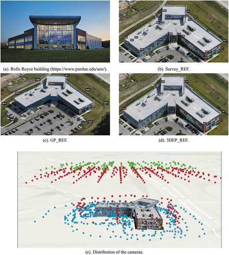
Figure 2. Devices used for image data acquisition (from left to right: iPhone 7, DJI Mavic 2 Pro, DJI Matrice 600, and a GPS ground panel that was used during the DJI Matrice 600 flight).

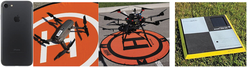
Table 1. Parameters of the three image datasets collected from a smartphone and drones for the Rolls Royce building.

Dataset	Device GPS Accuracy	# Images	Target	Observe distance	Image size	GSD	Focal length	Date (2020)
iPhone	1–8 m	466	Facade	~18 m	4032×3024	0.6 cm	4 mm	Apr.25
DJI Mavic 2 Pro	1–3 m	212 (oblique)	Facade	~15 m	5248×3936	0.4 cm	16 mm	July 1
		266 (vertical)	Roof	~43 m		1.4 cm
DJI Matrice 600	<0.1 m (PPK)	131 (vertical)	Roof	~49 m	6000×4000	1.1 cm	21 mm	July 7

The location and orientation of the M600 images were obtained through PPK. Detailed information on the number of images, initial sensor location accuracy, image dimension, Ground Sampling Distance (GSD), focal length, and dates of acquisition are listed in Table 1. The positioning accuracy of the onboard GPS/GNSS receivers ranges from 0.1–8 m, which will be used as direct geo-referencing information in bundle adjustment calculation.

In addition to the image datasets, three sets of ground control were acquired from a total station, an Indiana 3DEP lidar survey, and 10 ground GPS receivers. They are evenly distributed in the scene area shown in Figure 1. As shown in Figure 1(b), the first set (Survey_REF) was composed of four GCPs and 22 distinct features on the building measured by a Topcon ES total station (2 mm distance accuracy and 5“angle accuracy), with 10 on the roof edge and 12 on the facades. Four control points were set around the outer perimeter of the building. These control points were marked on the ground by survey nails drilled and set into the pavement. In accordance with standard closed-traversing procedures, each control point was occupied consecutively. At each station, the horizontal angle between the back station and forward station was observed in the “two-face” method which utilizes redundant angle measurement to remove the effect of systematic error in the angle observation. Additionally, the horizontal and vertical angles were recorded. Using this closed-traverse method allowed the error accumulated in the measurements to be calculated from the misclosure values. This error was then distributed using a least squares solution. Once the traverse was completed and adjusted, the coordinates of each station were calculated. To calculate the coordinates of a point on the building, the total station was set up on the recently established control points then the horizontal angle, vertical angle, and slope distance from the occupied control station were measured. From these measurements, the coordinates of the building point were found. To increase redundancy and to check for measurement errors, each point on the building was measured from a minimum of two control points.

Specifically used for the image dataset from DJI M600, the second ground control (GP_REF, Figure 1(c)) was collected during its flight by 10 evenly distributed Propeller Aeropoints, whose accuracy is up to 2 cm by the post-process technology (https://www.propelleraero.com/aeropoints/) with a government-operated Continuously Operating Reference Station (CORS) network. The third ground control (3DEP_REF, Figure 1(d)) was from the 2018 Indiana 3DEP airborne lidar data, which follows the specification of 10 cm non-vegetated height accuracy and two points per square meter point density. In this reference dataset, seven lidar points located on the roof eaves of the building are selected (four for control and three for check). These points were chosen because they occupy the same locations as the targets of the total station surveys. Due to the occlusion and sparse point density, several targets of the total station survey were not able to be located in 3DEP. The NAD83 (2011) UTM 16N and NAVD88 were utilized for each control implemented. Detailed information on the ground references considering the name, number of points, and sources are listed in Table 2. The distribution of these references is shown in Figure 1(b–d), where the background is dense point clouds respectively derived from oblique (Figure 1(c)) and vertical (Figure 1(b,d)) drone images. Figure 1(e) illustrates the spatial distribution of locations where images were taken using different platforms.

Table 2. Specifications of three ground reference datasets.

References	# Points	Source or Devices	Accuracy	Used for Control	Used for Check
Survey_REF	10 Roof (R)	Topcon ES Total Station	0.5 cm	R1, R3, R5, R7, R9	R2, R4, R6, R8, R10
	12 Facade (F)			F1, F10, F14, F16, F23, F28, F30	F2, F3, F18, F29, F31
GP_REF	10 (G)	Propeller Aeropoints GPS Panels	2 cm	G1, G3, G5, G7, G10	G2, G4, G6, G8, G9
3DEP_REF	7 (L)	2018 3DEP (lidar)	Vertical 10 cm	L1, L3, L6, L10	L2, L4, L7

4. Experiment and evaluation

Our workflow is embedded in Agisoft Metashape 1.8. The SfM includes feature extraction, feature matching, and bundle adjustment. While conducting camera calibration in the Metashape, all models assume a central projection frame camera with Brown’s distortion (Brown 1966). Since only the camera location and the focal length are given, the camera orientation and the interior parameters are initialized with zeros, which are then optimized through the bundle adjustment. In our experiment, the sensor models include the following parameters: focal length ($f$), principle point offset ($c_x$ and $c_y$), radial distortion coefficients ($k_1,\hspace{0.17em}{k}_2$, and $k_3$), and tangential distortion coefficients ($p_1$ and $p_2$).

The SfM procedure results in a sparse 3D point cloud of the building as well as the position and orientation of the cameras, while the dense matching procedure generates a much denser point cloud representing the scene. To evaluate the accuracy of direct geo-referencing, GNSS information from built-in/on-board sensors is first used to perform aero-triangulation. For comparison, ground control points have been introduced into the process, as well. The image coordinates of these ground references are manually identified, and the bundle adjustment process is conducted to simultaneously determine the position of the feature (tie) points along with the camera orientation and position. A total of 14 cases are conducted to evaluate the accuracy of SfM for different image datasets and their combination under various ground control schemes. The objective of using combined datasets is to achieve full coverage of the scene that is only partially covered by the vertical images or oblique images separately. At the end of this section, we also briefly evaluate the quality of the derived dense point clouds in terms of cloud-to-cloud distances, point density, and spacing.

4.1. Accuracy of individual image datasets

This section will examine the geometric quality of SfM for different image datasets under various ground control schemes. All evaluation (checking) is based on the field surveying points (Survey_REF), the most accurate ground reference we could achieve. As shown in Table 3, we initially used the built-in GNSS information of the smartphone for direct geo-referencing. When other ground control, such as 3DEP lidar data and Survey_REF, are introduced, the smartphone GNSS information is only used as the initial location for the SfM process. For all three control schemes introduced to the smartphone images (built-in GNSS, 3DEP, Survey), approximately $1.7\times {10}^5$ tie points are created from SfM. The positioning accuracy was evaluated by the ten checkpoints (listed in Table 2) in Survey_REF, five on the roof and five on the facades. Similarly, the DJI_MA2 drone’s positioning accuracy is listed in Table 4, where the same ground control schemes were used: built-in GNSS, 3DEP, and Survey. About $5.0\times {10}^5$ tie points were created from the DJI_MA2 oblique and vertical drone images in the SfM calculation.

Table 3. Position errors of smartphone image SfM under different ground control schemes (unit: cm).

Case	Case 1: iPhone (built-in GNSS)				Case 2: iPhone + 3DEP_REF				Case 3: iPhone + Survey_REF
Coord.	x	y	z	total	x	y	z	total	x	y	z	total
$\mathrm{m}\mathrm{e}\mathrm{a}\mathrm{n}$	−76.60	93.33	80.53	153.55	−20.69	2.84	−2.00	37.62	−0.57	−0.83	−1.63	12.43
$\mathrm{S}\mathrm{t}\mathrm{d}.\mathrm{D}\mathrm{e}\mathrm{v}$	56.32	49.18	26.67	61.54	29.88	20.16	11.62	21.43	10.82	7.04	6.36	7.50
$\mathrm{R}\mathrm{M}\mathrm{S}\mathrm{E}$	95.07	105.00	84.83	165.43	36.35	20.36	11.79	43.30	10.84	7.09	6.57	14.52

Table 4. Position errors of DJI_MA2 drone (both vertical and oblique) image SfM under different control schemes (unit: cm).

Case	Case 4: DJI_MA2 (built-in GNSS)				Case 5: DJI_MA2 + 3DEP_REF				Case 6: DJI_MA2 + Survey_REF
Coord.	x	y	z	total	x	y	z	total	x	y	z	total
$\mathrm{m}\mathrm{e}\mathrm{a}\mathrm{n}$	−123.92	64.64	−60.20	155.91	−11.57	4.51	3.95	20.05	0.89	−1.26	−0.39	3.46
$\mathrm{S}\mathrm{t}\mathrm{d}.\mathrm{D}\mathrm{e}\mathrm{v}$	25.31	21.02	25.26	23.99	9.72	13.95	3.55	8.32	1.16	1.65	2.69	1.38
$\mathrm{R}\mathrm{M}\mathrm{S}\mathrm{E}$	126.49	67.97	65.29	157.74	15.11	14.66	5.31	21.71	1.46	2.08	2.72	3.73

With respect to the quality of SfM from smartphone images, Table 3 illustrates that, when using only the GNSS information for geo-referencing, an overall positioning accuracy of 165.4 cm can be achieved. Despite this case having the greatest error, it is surprisingly better than expected, given that this involved the use of only a personal smartphone (iPhone 7). When 3DEP is used as a control, the positioning accuracy is improved to a sub-meter (43.3 cm). This is encouraging since such accuracy is close to the quality of 3DEP data (10 cm non-vegetated height accuracy and 30 cm point-spacing). Not surprisingly, the best accuracy of 14.5 cm, was achieved using survey ground control.

A similar analysis based on Table 4 can be made on the quality of SfM for the DJI_MA2 images. First, directly geo-referenced by the built-in GNSS information captured during the flight, the overall positioning accuracy of bundle adjustment for the drone images can achieve 157.7 cm. After introducing 3DEP as indirect geo-referencing, the positioning accuracy is enormously improved to 21.7 cm, which is equivalent to the quality of the 3DEP data. Among those geo-referencing methods, the result referenced by the field total station surveys achieves the best accuracy of 3.7 cm.

It is interesting to examine the SfM accuracy of the smartphone images and the one from the off-the-shelf DJI_MA2 images. When only direct geo-referencing is used, both datasets can achieve a meter-level positioning accuracy (165.4 cm for smartphone vs 157.7 cm for DJI_MA2). They are practical of equal quality. Using smartphone and drone images with only built-in GNSS as direct control is not sufficient for producing accurate 3D positions for urban infrastructures. When 3DEP is introduced as control, the geometric accuracy relation is changed to 43.3 vs 21.7 cm for smartphone vs drone, which implies that ground control, even though at a very coarse precision and resolution (such as 3DEP), can significantly improve the photogrammetry results from COTS images. Although the use of surveying points as ground control can significantly improve the SfM quality of DJI_MA2 images (from 21.7 to 3.7 cm), its contribution to smartphone images is less significant (from 43.3 to 14.5 cm). This is likely due to the intrinsic quality of the smartphone camera, whose distortion cannot be compensated by only using accurate ground control. The intrinsic uncertainty for smartphone images is likely at the magnitude of 10 cm, which is evidenced by the smallest SfM error of 12.4 ± 7.5 cm. In contrast, the DJI MA2 images, though also from an off-the-shelf camera, can benefit more from the high-quality ground control, leading to a position accuracy of several centimeters 3.5 ± 1.9 cm. Again, this can be regarded as the intrinsic uncertainty for the SfM with COTS DJI MA2 images.

Different from the other two image datasets, facades can hardly be observed in the images captured by DJI M600 due to its vertical view angle. The DJI M600 images can be directly controlled by the onboard PPK GPS receiver. Since most total station survey points (Survey_REF) are not visible in the DJI M600 images, only the ground GPS panels and the 3DEP aerial lidar data can be used as ground control for indirect geo-referencing. The SfM results for the DJI M600 images are listed in Table 5.

Table 5. Position errors of DJI M600 drone image SfM under different ground control sources (cm).

Case	Case 7: DJI_M600 (PPK GPS)				Case 8: DJI_M600 (PPK GPS) + 3DEP_REF
Coord.	x	y	z	total	x	y	z	total
$\mathrm{m}\mathrm{e}\mathrm{a}\mathrm{n}$	1.79	−3.12	2.05	8.54	1.39	−3.19	1.67	11.71
$\mathrm{S}\mathrm{t}\mathrm{d}.\mathrm{D}\mathrm{e}\mathrm{v}$	4.46	4.18	4.54	1.49	8.08	6.18	4.75	1.93
$\mathrm{R}\mathrm{M}\mathrm{S}\mathrm{E}$	4.81	5.21	4.99	8.67	8.20	6.96	5.04	11.87
Case	Case 9: DJI_M600 (PPK GPS) + GP_REF				Case 10: DJI_M600 + GP_REF
Coord.	x	y	z	total	x	y	z	total
$\mathrm{m}\mathrm{e}\mathrm{a}\mathrm{n}$	−0.99	0.06	−1.18	4.37	−0.79	0.62	−1.46	3.93
$\mathrm{S}\mathrm{t}\mathrm{d}.\mathrm{D}\mathrm{e}\mathrm{v}$	2.69	1.85	2.73	1.19	2.50	1.18	2.53	1.32
$\mathrm{R}\mathrm{M}\mathrm{S}\mathrm{E}$	2.87	1.85	2.98	4.53	2.62	1.34	2.92	4.14

Compared to the built-in GNSS SfM errors in Tables 3 and 4, a positioning accuracy of around 8.5 ± 1.5 cm (case 7) is achieved by PPK GPS geo-referencing in Table 5. This level of accuracy is the best among all of the direct geo-referencing SfM results. The result is reasonable since many references report PPK for drone flight can achieve an accuracy of several centimeters (Hill 2019). Compared to the other two sensors (smartphone and DJI MA2), the quality of the professional sensor and platform with PPK capability is significantly superior (8.7 vs 165.4 and 157.7 cm respectively for iPhone and DJI MA2). However, when 3DEP data is introduced together with the onboard PPK GPS as control (case 8), the accuracy of SfM of DJI M600 images is 11.7 ± 1.9 cm. This is not a surprise since the quality of 3DEP data is over 5 times worse than the PPK GPS data. Despite such quality differences considered during bundle adjustment, the adverse contribution of 3DEP data does not fully vanish. Similarly, we introduce the GPS panel as control together with the PPK GPS (case 9), the SfM of DJI M600 images can achieve a positioning accuracy of 4.4 ± 1.2 cm, an improvement of a factor of two when compared with the results of only using onboard PPK GPS (case 7). Finally, test case 10 intends to demonstrate the scenario when the PPK GPS is not available or not included as control and the control is only from GPS panels on the ground. In this situation, the SfM of DJI M600 images achieves the best accuracy of 3.9 ± 1.3 cm, which is comparable with the CORS-corrected quality of these GPS panels. When this result from GPS panel control is compared with the ones in Table 4, the accuracy is comparable but barely as good as the one from DJI MA2 images (3.7 cm) due to the higher-flying height of DJI M600 and the finer resolution of DJI MA2 oblique images (see Table 1).

The above experiments demonstrate that the positioning accuracy of smartphone and COTS drone SfM with simple (without PPK) onboard GPS geo-referencing ranges from 157.7–165.4 cm. After introducing 3DEP aerial lidar data as geo-references, the positioning accuracy of 21.7–43.3 cm can be achieved, which is rather consistent with the intrinsic quality of the 3DEP reference data. When traditional total station surveying or precise GPS surveying is used as control, the COTS drone (DJI MA2) and professional drone (DJI M600) can achieve practically equivalent accuracy (3.7 vs 4.1 cm or 2.6 vs 3.7 GSD), which is comparable with the best quality of GPS surveying technology, demonstrating the promising potential of low-end drone images as a replacement of professional ones, considering their significant cost difference and similar geometric accuracy. On the other hand, the ground GPS panels are easier to deploy, and observation of GPS signals for~40 min is about the same as drone flight. As such, creating accurate ground control of centimeter accuracy with precise GPS techniques does not necessarily take extra time for a project. However, it is not convenient to deploy such GPS panels on top of the roof. As such, the corresponding SfM may lack vertical control when the panels are only distributed on the ground. This is the situation in this study, where the 2.9 cm height error (Table 5) is slightly inferior to the best of 2.7 cm (Table 4) obtained with the DJI MA2 and Survey_REF combination. Professional drones (e.g. DJI M600) with PPK GPS capabilities can achieve a direct geo-referencing accuracy of 8.7 cm, which can be improved by a factor of two when precise ground control from either GPS panels or surveying is used as a sole or additional control.

4.2. Accuracy of combined image datasets

In section 4.1, we demonstrate the best accuracy one can expect from smartphone images as a major data source. However, rooftops are not visible in the smartphone imagery. The opposite situation may occur for vertically captured drone images since the building walls can hardly be observed at a nadir angle. Hence, it is necessary to explore the performance of SfM from a combined dataset consisting of both oblique and vertical images, likely from different sensors. The accuracy of those cases is evaluated by the same 10 total station surveyed checkpoints used in the previous cases. The results of SfM for the combined datasets under different ground control schemes are listed in Table 6.

Table 6. Position errors of SfM for combined image datasets under different ground control sources (unit: cm).

Case	Case 11: iPhone + DJI_M600 + GP_REF				Case 12: iPhone + DJI_MA2 (vertical) + Survey_REF
Coord.	x	y	z	total	x	y	z	total
$\mathrm{m}\mathrm{e}\mathrm{a}\mathrm{n}$	0.14	−0.66	0.01	3.48	0.11	0.51	−0.21	2.74
$\mathrm{S}\mathrm{t}\mathrm{d}.\mathrm{D}\mathrm{e}\mathrm{v}$	0.99	1.36	3.59	2.02	1.45	1.88	1.79	1.29
RMSE	1.01	1.51	3.59	4.01	1.46	1.95	1.81	3.03
Case	Case 13: DJI_MA2 (oblique) + DJI_M600 + GP_REF				Case 14: DJI_MA2 (oblique) + DJI_M600 + Survey_REF
Coord.	x	y	z	total	x	y	z	total
$\mathrm{m}\mathrm{e}\mathrm{a}\mathrm{n}$	0.26	0.56	1.67	4.52	0.69	−0.5	−0.39	2.11
$\mathrm{S}\mathrm{t}\mathrm{d}.\mathrm{D}\mathrm{e}\mathrm{v}$	1.96	0.71	4.24	2.24	0.63	1.22	1.52	0.80
RMSE	1.98	0.90	4.56	5.05	0.94	1.32	1.57	2.26

As stated earlier in the data acquisition section, only the DJI MA2 collected both vertical and oblique images for the building. In contrast, the DJI M600 only collected vertical images, whereas the smartphone images were collected from the ground and thus only cover walls. We first apply SfM to the combined datasets of the DJI MA2 oblique and DJI M600 images. Similarly, the combined datasets of smartphone images respectively with DJI MA2 (vertical) and DJI M600 images are also used as input for SfM. Since ground GPS panels were only observed on DJI M600 images, they could not be used to control other images.

Table 6 demonstrates that the combination (cases 11 and 12) of smartphone images with drone (vertical) images, either low-end or high-end, can achieve the same quality level (3.0–4.0 cm), which is slightly better than the results from only one dataset, cases 6 and 10 (3.7–4.1 cm). This implies that the inclusion of smartphone images can not only make possible the facade mapping, but in the meantime increase the accuracy of structure from motion through combined bundle adjustment. Having observed this comparison, it can be concluded that smartphone images can be used to replace drone oblique images (DJI MA2) for SfM while achieving an accuracy of up to 20% better (from 3.0 vs 3.7 cm to 4.0 vs 4.1 cm), which mostly comes from the large number of smartphone images involved (466). This finding is beneficial since operating drones for oblique imaging over walls is extremely time-consuming and consumes most of the time for drone data acquisition unless advanced navigation and flight planning capability are available.

Test cases 13 and 14 are for the combination of DJI MA2 oblique images with DJ M600 images under different ground control schemes. Unsurprisingly, the best accuracy (2.3 cm) is achieved by using the total station survey as a means of ground control. The major difference between GPS panels (case 13) and the total station survey (case 10) is that the former is a lack of control in the vertical direction, where the major deficiency (4.6 vs 1.6 cm) occurs, leading to a worse total positioning accuracy (5.0 cm vs 4.1 cm). Based on the findings above, it is evident that the combination of these two complementary datasets is beneficial in keeping the positioning accuracy at a centimeter level, resulting in a more integral building model than individual datasets could achieve separately.

4.3. Quality of the point clouds

After bundle adjustment in SfM, dense image matching is then carried out. Since the focus of the work is on geometric accuracy, we will only briefly investigate the quality (relative accuracy) of the point clouds as a result of dense matching.

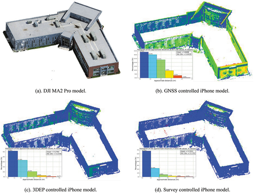
We first calculate the cloud-to-cloud distances for the point clouds derived from iPhone images under different control schemes, i.e. built-in GNSS, 3DEP, and survey. Figure 3 shows the distribution of such cloud-to-cloud distances. The reference point cloud shown in Figure 3(a) is taken as the one derived from the DJI MA2 Pro images under the control of the total station measurements (Survey_REF). The average cloud-to-cloud distance is 0.61 m when controlled by the built-in GNSS (Figure 3(b)), and is respectively reduced to 0.09 m and 0.04 m after referenced by 3DEP (Figure 3(c)) and survey points (Figure 3(d)).

Figure 3. Distributions of the cloud-to-cloud distances of the iPhone created models with reference to the one created from the total station controlled DJI MA2 Pro. The DJI MA2 Pro derived point cloud (a) and colored coded cloud-to-cloud distances between the iPhone point clouds respectively under the control of GNSS (b), 3DEP (c), and survey (d), with reference to the DJ2 MA2 Pro point cloud.

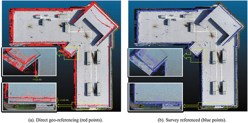
Such cloud-to-cloud distances can be further explored under the context of the imaged target. We notice some significant misalignment in the smartphone-derived point cloud from direct geo-referencing with the built-in GNSS information. By overlapping the smartphone-derived dense points (red points) under direct geo-referencing with the ones derived from the oblique drone images referenced to the total station survey, we can observe an apparent misalignment (Figure 4(a)). Such misalignments are at the magnitude of 1.6 m as listed in Table 3 and systematically toward west-north. This can be corrected to 14 cm (blue points in Figure 4(b)) by introducing the total station survey as the reference during bundle adjustment (Figure 4(b)).

Figure 4. Overlap of the smartphone dense point clouds referenced by the built-in GPS receiver ((a) Red points) and the total station survey ((b) Blue points). A 1.6 m misalignment can be observed. The background is the total station controlled DJI MA2 oblique drone-derived dense point clouds.

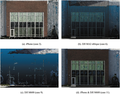
Point density and spacing are two basic metrics for the quality of point clouds. Point density refers to the number of points per unit area. However, since smartphone images or oblique images can only be used to reconstruct facades, we use point spacing as an additional metric to describe the quality of point clouds. Four resultant dense point clouds are considered for our discussion: smartphone (case 3), DJI MA2 oblique (case 6), DJI M600 (case 9), and combined smartphone with DJI M600 (case 11). The 2D point density and the 3D point spacing for the aforementioned experiment cases are computed and listed in Table 7. This table shows that, under the same dense matching parameters, drone imagery can derive dense point clouds with an average point spacing of 3.4 cm and an average density of ~ 470 pts/${\mathrm{m}}^2$. In contrast, smartphone images can achieve a much smaller point spacing of 0.8 cm. For the combined dataset of smartphone and DJI M600 images, the point density is changed to 2.0 cm. It is interesting to note that the low-end drone and high-end drone produce similar point density (497 vs 441 pts/m2) and point spacing (3.3 vs 3.5 cm) for the derived point clouds. Among the mentioned experiments, the smartphone can derive the densest and thickest point clouds and can be used to enrich the drone dense matching result by 2.7 times.

Table 7. Number of points, point density, and 3D point spacing of dense point clouds.

Case (3,6,9,11)	iPhone	DJI MA2 (oblique)	DJI M600	iPhone + DJI M600
Number of points	7,948,918	3,353,202	2,972,470	10,953,427
2D point density (unit: pts/m^2)	1182.94	497.63	441.04	1439.18
3D point spacing (unit: cm)	0.8	3.3	3.5	2.0

To examine the details of the created point clouds, we show the point distribution for the north facade of the building. The dense point cloud from smartphone images (Figure 5(a)) is significantly denser than the one from oblique drone images (Figure 5(b)). Though the facades are hardly observable in the high-end DJI M600 drone images (Figure 5(c)), this situation can be resolved by combining them with the smartphone images (Figure 5(d)).

Figure 5. Point density visualization of the dense point clouds of a north facade derived from iPhone (a), DJI MA2 oblique (b), DJI M600 vertical (c), and iPhone and DJI M600 combined (d). Note that the point size of the above point clouds is consistent.

5. Conclusions

We assessed the best performance of SfM conducted with COTS sensors, such as smartphones and off-the-shelf drones, by evaluating 14 test cases derived from various sensors and referenced under different control schemes. The experiment results show that the positioning accuracy of smartphone images under direct geo-referencing is 165.4 cm and can be improved to 43.3 cm and 14.5 cm when introducing the 3DEP aerial lidar data and total station surveys as controls, respectively. Similar results were found for low-end DJI MA2 drone images as well. By introducing the 3DEP lidar data, the positioning accuracy of the COTS sensors can be improved to a quality of 20–30 cm, close to the quality of the 3DEP control data. The best SfM results (3.7 cm and 4.1 cm or 2.6 vs 3.7 GSD) of drones can be achieved by referencing the images with expensive and time-consuming total station surveying or GPS surveying. The combination of smartphone images with drone (vertical) images, either low-end or high-end, can achieve about the same quality level (3.0–4.0 cm), which is slightly better than the results from only one dataset (3.7–4.1 cm), implying that smartphone images can be used to replace drone oblique images with an improved accuracy due to the large number of smartphone images involved. Professional drones with PPK GPS capability can achieve an SfM accuracy of 8.7 cm (7.9 GSD), which can be further improved by using independent field surveying quality control. Furthermore, caution needs to be exercised when control information of different qualities needs to be jointly used; properly weighting is necessary to achieve the best outcome.

For future work, we suggest more experiments be conducted to explore the proper number of images, distance from the camera to the objects, and especially newer brands of smartphones for achieving the optimal SfM results. Though the great potential is shown by introducing the aerial lidar as cost-free control into drone and smartphone SfM, issues like sparsity and omission while picking reference points in the lidar point cloud still exist, which results in uncertainty in the outcome. Hence, research considering the methods of selecting accurate reference points from lidar point clouds shall be explored. We also recommend more investigations about combining smartphone and drone images under different illuminant conditions and resolutions to assure the best SfM outcome. Finally, smartphone images alone can hardly achieve an accuracy of centimeter-level due to their intrinsic camera distortions. While using newer generation off-the-shelf smartphones will certainly yield more accurate results, their camera distortion models shall also be investigated to maximize the potential of such handheld ubiquitous sensors.

Disclosure statement

No potential conflict of interest was reported by the author(s).

Data availability statement

The data used in this study is currently not available for public use.

Additional information

Notes on contributors

Jie Shan

Jie Shan conceptualization, supervision, fieldwork, analysis, writing.

Zhixin Li

Zhixin Li field surveying, fieldwork, data curation, photogrammetric experiments, writing.

Damon Lercel

Damon Lercel drone data acquisition, writing.

Kevan Tissue

Kevan Tissue filed surveing and computation, smartphone image acquisition and curation, writing.

Joseph Hupy

Joseph Hupy drone data acquistion, writing.

Joshua Carpenter

Joshua Carpenter field surveying, writing.

References

- Ackermann, F. 1987. “The Use of Camera Orientation Data in Photogrammetry – A Review.” Photogrammetry 42 (1–2): 19–33. doi:10.1016/0031-8663(87)90003-2.
- Ackermann, F. 1992a. “Operational Rules and Accuracy Models for GPS-Aerotriangulation.” Arch. ISPRS 1: 691–700.
- Ackermann, F. 1992b. “Prospects of Kinematic GPS for Aerial Triangulation.” ITC Journal 4: 326–338.
- Ackermann, F. 1996. “Photogrammetry Today.” ITC Journal 3 (4): 230–237.
- Agüera-Vega, F., F. Carvajal-Ramírez, and P. Martínez-Carricondo. 2017. “Assessment of Photogrammetric Mapping Accuracy Based on Variation Ground Control Points Number Using Unmanned Aerial Vehicle.” Measurement 98: 221–227. doi:10.1016/j.measurement.2016.12.002.
- Baqersad, J., P. Poozesh, C. Niezrecki, and P. Avitabile. 2017. “Photogrammetry and Optical Methods in Structural Dynamics – A Review.” Mechanical Systems and Signal Processing 86: 17–34. doi:10.1016/j.ymssp.2016.02.011.
- Brown, D. C. 1966. “Decentering Distortion of Lenses. Photogrammetric Engineering and Remote Sensing.” https://ci.nii.ac.jp/naid/10022411406/
- Caldera-Cordero, J. M., and M.-E. Polo. 2019. “Analysis of Free Image-Based Modeling Systems Applied to Support Topographic Measurements.” Survey Review 51 (367): 300–309. doi:10.1080/00396265.2018.1451271.
- Chen, B., C. Gao, Y. Liu, and P. Sun. 2019. “Real-Time Precise Point Positioning with a Xiaomi MI 8 Android Smartphone.” Sensors 19 (12): 2835. doi:10.3390/s19122835.
- Chirico, P., J. DeWitt, and S. Bergstresser. 2020. “Evaluating Elevation Change Thresholds Between Structure-From-Motion DEMs Derived from Historical Aerial Photos and 3DEP LiDar Data.” Remote Sensing 12 (10): 1625. doi:10.3390/rs12101625.
- Duró, G., A. Crosato, M. G. Kleinhans, and W. S. J. Uijttewaal. 2018. “Bank Erosion Processes Measured with UAV-Sfm Along Complex Banklines of a Straight Mid-Sized River Reach.” Earth Surface Dynamics 6 (4): 933–953. doi:10.5194/esurf-6-933-2018.
- Ferrer-González, E., F. Agüera-Vega, F. Carvajal-Ramírez, and P. Martínez-Carricondo. 2020. “UAV Photogrammetry Accuracy Assessment for Corridor Mapping Based on the Number and Distribution of Ground Control Points.” Remote Sensing 12 (15): 2447. doi:10.3390/rs12152447.
- Gerke, M., and H.-J. Przybilla. 2016. “Accuracy Analysis of Photogrammetric UAV Image Blocks: Influence of Onboard RTK-GNSS and Cross Flight Patterns.” Photogrammetrie, Fernerkundung, Geoinformation 2016: 17–30. doi:10.1127/pfg/2016/0284.
- Grenzdörffer, G. J., M. Naumann, F. Niemeyer, and A. Frank. 2015. “Symbiosis of Uas Photogrammetry and Tls for Surveying and 3d Modeling of Cultural Heritage Monuments - A Case Study About the Cathedral of ST. Nicholas in the City of Greifswald.” ISPRS - International Archives of the Photogrammetry, Remote Sensing and Spatial Information Sciences XL1: 91. doi:10.5194/isprsarchives-XL-1-W4-91-2015.
- Hansman, R. J., and U. Ring. 2019. “Workflow: From Photo-Based 3-D Reconstruction of Remotely Piloted Aircraft Images to a 3-D Geological Model.” Geosphere 15 (4): 1393–1408. doi:10.1130/GES02031.1.
- Havlena, M., and K. Schindler. 2014. “VocMatch: Efficient Multiview Correspondence for Structure from Motion.” Computer Vision – ECCV 2014: 46–60. doi:10.1007/978-3-319-10578-9_4.
- Hill, A. C. 2019. “Economical Drone Mapping for Archaeology: Comparisons of Efficiency and Accuracy.” Journal of Archaeological Science: Reports 24: 80–91. doi:10.1016/j.jasrep.2018.12.011.
- Hupy, J. P., and C. Wilson. 2021. “Modeling Streamflow and Sediment Loads with a Photogrammetrically Derived UAS Digital Terrain Model: Empirical Evaluation from a Fluvial Aggregate Excavation Operation.” Drones 5 (1): 20. doi:10.3390/drones5010020.
- Iheaturu, C. J., E. G. Ayodele, and C. J. Okolie. 2020. “An Assessment of the Accuracy of Structure-From-Motion (SfM) Photogrammetry for 3D Terrain Mapping.” Geomatics, Landmanagement and Landscape 65–82. doi:10.15576/GLL/2020.2.65.
- Jiang, S., C. Jiang, and W. Jiang. 2020. “Efficient Structure from Motion for Large-Scale UAV Images: A Review and a Comparison of SfM Tools.” ISPRS Journal of Photogrammetry and Remote Sensing 167: 230–251. doi:10.1016/j.isprsjprs.2020.04.016.
- Kang, L., L. Wu, and Y.-H. Yang. 2014. “Robust Multi-View L2 Triangulation via Optimal Inlier Selection and 3D Structure Refinement.” Pattern Recognition 47 (9): 2974–2992. doi:10.1016/j.patcog.2014.03.022.
- Lercel, D. J., and J. P. Hupy. 2020. “Developing a Competency Learning Model for Students of Unmanned Aerial Systems.” Collegiate Aviation Review International 38 (2): 12–33. doi:10.22488/okstate.20.100212.
- Lowe, D. G. 2004. “Distinctive Image Features from Scale-Invariant Keypoints.” International Journal of Computer Vision 60 (2): 91–110. doi:10.1023/B:VISI.0000029664.99615.94.
- Magri, L., and R. Toldo. 2017. “Bending the Doming Effect in Structure from Motion Reconstructions Through Bundle Adjustment.” ISPRS - International Archives of the Photogrammetry Remote Sensing and Spatial Information Sciences 42: 235–241. doi:10.5194/isprs-archives-xlii-2-w6-235-2017.
- Marr, D., and T. Poggio. 1976. “Cooperative Computation of Stereo Disparity.” Science 194 (4262): 283–287. doi:10.1126/science.968482.
- Martínez-Carricondo, P., F. Agüera-Vega, F. Carvajal-Ramírez, F.-J. Mesas-Carrascosa, A. García-Ferrer, and F.-J. Pérez-Porras. 2018. “Assessment of UAV-Photogrammetric Mapping Accuracy Based on Variation of Ground Control Points.” International Journal of Applied Earth Observation and Geoinformation 72: 1–10. doi:10.1016/j.jag.2018.05.015.
- Mercuri, M., K. J. W. McCaffrey, L. Smeraglia, P. Mazzanti, C. Collettini, and E. Carminati. 2020. “Complex Geometry and Kinematics of Subsidiary Faults Within a Carbonate-Hosted Relay Ramp.” Journal of Structural Geology 130 (103915): 103915. doi:10.1016/j.jsg.2019.103915.
- Mlambo, R., I. Woodhouse, F. Gerard, and K. Anderson. 2017. “Structure from Motion (SfM) Photogrammetry with Drone Data: A Low Cost Method for Monitoring Greenhouse Gas Emissions from Forests in Developing Countries.” Forests 8 (3): 68. doi:10.3390/f8030068.
- Mohan, A., and S. Poobal. 2018. “Crack Detection Using Image Processing: A Critical Review and Analysis.” Alexandria Engineering Journal 57 (2): 787–798. doi:10.1016/j.aej.2017.01.020.
- Murtiyoso, A., and P. Grussenmeyer. 2017. “Documentation of Heritage Buildings Using Close-Range UAV Images: Dense Matching Issues, Comparison and Case Studies.” Photogrammetric Record 32: 206–229. doi:10.1111/phor.12197.
- Murtiyoso, A., M. Koehl, P. Grussenmeyer, and T. Freville. 2017. “Acquisition and Processing Protocols for Uav Images: 3d Modeling of Historical Buildings Using Photogrammetry.” ISPRS Annals of Photogrammetry, Remote Sensing & Spatial Information Sciences 4W (2): 163–170. doi:10.5194/isprs-annals-IV-2-W2-163-2017.
- Nex, F., and F. Remondino. 2014. “UAV for 3D Mapping Applications: A Review.” Applied Geomatics 6 (1): 1–15. doi:10.1007/s12518-013-0120-x.
- Oh, S., J. Jung, G. Shao, G. Shao, J. Gallion, and S. Fei. 2022. “High-Resolution Canopy Height Model Generation and Validation Using USGS 3DEP LiDar Data in Indiana, USA.” Remote Sensing 14 (4): 935. doi:10.3390/rs14040935.
- Oniga, V.-E., A.-I. Breaban, N. Pfeifer, and C. Chirila. 2020. “Determining the Suitable Number of Ground Control Points for UAS Images Georeferencing by Varying Number and Spatial Distribution.” Remote Sensing 12 (5): 876. doi:10.3390/rs12050876.
- Padró, J.-C., F.-J. Muñoz, J. Planas, and X. Pons. 2019. “Comparison of Four UAV Georeferencing Methods for Environmental Monitoring Purposes Focusing on the Combined Use with Airborne and Satellite Remote Sensing Platforms.” International Journal of Applied Earth Observation and Geoinformation 75: 130–140. doi:10.1016/j.jag.2018.10.018.
- Park, J. W., and D. J. Yeom. 2022. “Method for Establishing Ground Control Points to Realize UAV-Based Precision Digital Maps of Earthwork Sites.” Journal of Asian Architecture and Building Engineering 21 (1): 110–119. doi:10.1080/13467581.2020.1869023.
- Pierdicca, R. 2018. “Mapping Chimu’s Settlements for Conservation Purposes Using UAV and Close Range Photogrammetry. The Virtual Reconstruction of Palacio Tschudi, Chan, Peru.” Digital Applications in Archaeology and Cultural Heritage 8: 27–34. doi:10.1016/j.daach.2017.11.004.
- Robustelli, U., V. Baiocchi, and G. Pugliano. 2019. “Assessment of Dual Frequency GNSS Observations from a Xiaomi Mi 8 Android Smartphone and Positioning Performance Analysis.” Electronics 8 (1): 91. doi:10.3390/electronics8010091.
- Sanz-Ablanedo, E., J. Chandler, J. Rodríguez-Pérez, and C. Ordóñez. 2018. “Accuracy of Unmanned Aerial Vehicle (UAV) and SfM Photogrammetry Survey as a Function of the Number and Location of Ground Control Points Used.” Remote Sensing 10 (10): 1606. doi:10.3390/rs10101606.
- Sapirstein, P. 2018. “A High-Precision Photogrammetric Recording System for Small Artifacts.” Journal of Cultural Heritage 31: 33–45. doi:10.1016/j.culher.2017.10.011.
- Schonberger, J. L., A. C. Berg, and J.-M. Frahm. 2015. “Paige: Pairwise Image Geometry Encoding for Improved Efficiency in Structure-From-Motion.” In Proceedings of the IEEE Conference on Computer Vision and Pattern Recognition, 1009–1018. doi:10.1109/CVPR.2015.7298703.
- Schönberger, J. L., and J.-M. Frahm. 2016. “Structure-From-Motion Revisited.” Proceedings of the IEEE Conference on Computer Vision and Pattern Recognition, 4104–4113. doi:10.1109/CVPR.2016.445.
- Shan, J. 2018. “A Brief History and Essentials of Bundle Adjustment.” Geomatics and Information Science of Wuhan University 43 (12): 1797–1810. doi:10.13203/j.whugis20180331.
- Snavely, N., I. Simon, M. Goesele, R. Szeliski, and S. M. Seitz. 2010. “Scene Reconstruction and Visualization from Community Photo Collections.” Proceedings of the IEEE 98 (8): 1370–1390. doi:10.1109/JPROC.2010.2049330.
- Su, W., M. Zhang, D. Bian, Z. Liu, J. Huang, W. Wang, J. Wu, and H. Guo. 2019. “Phenotyping of Corn Plants Using Unmanned Aerial Vehicle (UAV) Images.” Remote Sensing 11 (17): 2021. doi:10.3390/rs11172021.
- Tavani, S., A. Corradetti, P. Granado, M. Snidero, T. D. Seers, and S. Mazzoli. 2019. “Smartphone: An Alternative to Ground Control Points for Orienting Virtual Outcrop Models and Assessing Their Quality.” Geosphere 15 (6): 2043–2052. doi:10.1130/GES02167.1.
- Tavani, S., A. Pignalosa, A. Corradetti, M. Mercuri, L. Smeraglia, U. Riccardi, T. Seers, T. Pavlis, and A. Billi. 2020. “Photogrammetric 3D Model via Smartphone GNSS Sensor: Workflow, Error Estimate, and Best Practices.” Remote Sensing 12 (21): 3616. doi:10.3390/rs12213616.
- Teunissen, P. J. G., and O. Montenbruck. 2017. Springer Handbook of Global Navigation Satellite Systems. Cham: Springer. doi:10.1007/978-3-319-42928-1.
- Tian, X., Y. Xu, F. Wei, O. Gungor, Z. Li, C. Wang, S. Li, and J. Shan. 2020. “Pavement Macrotexture Determination Using Multi-View Smartphone Images.” Photogrammetric Engineering & Remote Sensing 86 (10): 643–651. doi:10.14358/PERS.86.10.643.
- Triggs, B., P. F. McLauchlan, R. I. Hartley, and A. W. Fitzgibbon. 2000. “Bundle Adjustment — A Modern Synthesis.” In Vision Algorithms: Theory and Practice, 298–372. Springer Berlin Heidelberg. doi:10.1007/3-540-44480-7_21.
- Tuytelaars, T., and K. Mikolajczyk. 2008. “Local Invariant Feature Detectors: A Survey.” Foundations and trends® in Computer Graphics and Vision 3 (3): 177–280. doi:10.1561/0600000017.
- Ullman, S. 1979. “The Interpretation of Visual Motion.” Massachusetts Inst of Technology Pr. 229. https://psycnet.apa.org/fulltext/1980-70610-000.pdf
- Westoby, M. J., J. Brasington, N. F. Glasser, M. J. Hambrey, and J. M. Reynolds. 2012. ““Structure-From-Motion” Photogrammetry: A Low-Cost, Effective Tool for Geoscience Applications.” Geomorphology 179: 300–314. doi:10.1016/j.geomorph.2012.08.021.
- Woodget, A. S., R. Austrums, I. P. Maddock, and E. Habit. 2017. “Drones and Digital Photogrammetry: From Classifications to Continuums for Monitoring River Habitat and Hydromorphology.” Wiley Interdisciplinary Reviews: Water 4 (4): e1222. doi:10.1002/wat2.1222.
- Wróżyński, R., K. Pyszny, M. Sojka, C. Przybyła, and S. Murat-Błażejewska. 2017. “Ground Volume Assessment Using ’Structure from Motion’ Photogrammetry with a Smartphone and a Compact Camera.” Open Geosciences 9 (1): 281–294. doi:10.1515/geo-2017-0023.
- Zhang, H., E. Aldana-Jague, F. Clapuyt, F. Wilken, V. Vanacker, and K. Van Oost. 2019. “Evaluating the Potential of Post-Processing Kinematic (PPK) Georeferencing for UAV-Based Structure- From-Motion (SfM) Photogrammetry and Surface Change Detection.” Earth Surface Dynamics 7: 807–827. doi:10.5194/esurf-7-807-2019.