A curvature-driven cloud removal method for remote sensing images

ABSTRACT

Cloud coverage has become a significant factor affecting the availability of remote-sensing images in many applications. To mitigate the adverse impact of cloud coverage and recover ground information obscured by clouds, this paper presents a curvature-driven cloud removal method. Considering that each image can be regarded as a curved surface and the curvature can reflect the texture information well due to its dependence on the surface’s undulation degree, the presented method transforms image from natural domain to curvature domain for information reconstruction to maintain details of reference image. In order to improve the overall consistency and continuity of cloud removal results, the optimal boundary for cloud coverage area replacement is determined first to make the boundary pass through pixels with minimum curvature difference. Then, the curvature of missing area is reconstructed based on the curvature of reference image, and the reconstructed curvature is inversely transformed to natural domain to obtain a cloud-free image. In addition, considering the possible significant radiometric differences between different images, the initial cloud-free result will be further refined based on specific checkpoints to improve the local accuracy. To evaluate the performance of the proposed method, both simulated experiments and real data experiments are carried out. Experimental results show that the proposed method can achieve satisfactory results in terms of radiometric accuracy and consistency.

KEYWORDS:

• Cloud removal
• curvature domain
• boundary optimization
• checkpoints refinement

1. Introduction

Remote-sensing images have already got popular use in many aspects, including environmental monitoring, disaster management, and smart city construction (Li et al. 2013; Li, Wang, and Jiang 2021). However, the existence of clouds in remote-sensing images has been a critical obstacle that reduces the spatio-temporal availability of ground surface observation, and further severely limits the applications of remote-sensing images. A study has shown that 67% of the Earth’s surface is obscured by clouds on average (King et al. 2013), and approximately 35% of land surface is covered by clouds (Ju and Roy 2008). Therefore, it is necessary to recover the missing area obscured by clouds in cloud-contaminated image, i.e. cloud removal (Fang et al. 2021).

In the last few decades, various methods including deep learning methods and non-deep learning methods have been presented for the task of cloud removal in optical data. Unlike deep learning methods, non-deep learning methods usually do not require a large amount of labeled data for training. According to the different sources of auxiliary information for cloud removal, these non-deep learning methods can be classified into three categories: spatial-based methods, multispectral-based methods, and multitemporal-based methods (Cheng et al. 2014; Shen et al. 2015). In spatial-based methods, the main idea is to reconstruct the ground information based on the pixels outside the cloud coverage area in cloud-contaminated image, and the most common one is missing pixel interpolation, including traditional interpolation methods, such as nearest-neighbor and bilinear resampling (Atkinson, Curran, and Webster 1990), and geostatistics interpolation methods, such as Kriging interpolation (Rossi, Dungan, and Beck 1994). These interpolation methods are mainly suitable for processing images with simple ground features, because most of them cannot make good use of the spatial information. In addition to interpolation methods, the exemplar-based method (Criminisi, Perez, and Toyama 2004), the variation-based method (Shen and Zhang 2009), and the propagated diffusion method (Maalouf et al. 2009) are also presented. In most cases, these methods can work better than interpolation methods. However, since the main idea of spatial-based methods is to utilize the spatial correlations in image, they may not be suitable for images with complex ground features (Guillemot and Le Meur 2014). Furthermore, with the increase of the size of cloud coverage area, the reconstruction accuracy may decrease significantly due to the insufficient prior information.

The multispectral-based methods are mainly used for multispectral and hyperspectral images. Since the band with longer wavelength has more powerful ability of penetrating through cloud (Kulkarni and Rege 2020), the cloud coverage areas in multispectral and hyperspectral images can be removed with the information from the unaffected band. For example, to detect the haze/cloud spatial distribution and recover the missing area in cloud-contaminated images, Zhang, Guindon, and Cihlar (2002) studied the spectral response characteristics under cloudy or clear-sky conditions and developed a haze optimized transformation model. Feng et al. (2004) regarded clouds as one of the common noises in images and proposed an improved homomorphism filtering method to remove thin clouds in ASTER images. Wang et al. (2005) used a mixing method of wavelet frequency analysis and B-spline based model to filter out the clouds in infrared band and repair the residual holes in other bands. In addition, some multispectral-based methods developed for the dead pixel completion and destriping are also used for cloud removal (Shen, Zeng, and Zhang 2011; Gladkova et al. 2012; Li et al. 2014). In general, the multispectral-based methods can work well for images with thin clouds.

The multitemporal-based methods are the most commonly used method, which utilize images acquired in the same area at different time to recover the missing information in cloud-contaminated image (Zhang et al. 2021). Due to the complete auxiliary information in multitemporal images, these methods can achieve a reliable result even for images with large and thick clouds (Cheng et al. 2014). The simple way is to directly replace the cloud coverage area in cloud-contaminated image with the same area in reference image. For a temporal sequence of images, Li et al. (2003) first sorted images according to the quality of the corresponding area in the multitemporal images, and then replaced the missing area with the optimal patch. Moreover, a pixel-based replacement method is also presented for large-scale cloud-free mosaic production (Kang et al. 2016). The direct replacement methods are simple and easy to implement, but they are not applicable when the radiometric differences between images are significant. Therefore, to reduce the radiometric differences between images, Helmer and Ruefenacht (2005) applied the improved histogram matching to adjacent scenes, and then used regression trees to predict the missing information obscured by clouds. Considering possible land changes between multi-temporal images, Meng et al. (2019) adopted a sliding window-based local matching algorithm to remove thin clouds and shadows while image pansharpening. Inspired by Poisson editing theory (Perez, Gangnet, and Blake 2003), many seamless cloning approaches for cloud removal have also been put forward, in which the gradient field of reference image is taken as the guidance vector field for information reconstruction. For example, Lai and Lin (2012) introduced the boundary optimization process on the basis of Poisson blending, and used the non-feature pixels to build a new boundary with minima gradient cost for cloud removal. Lin et al. (2013) used the temporal correlations of multitemporal images and reconstructed the missing information based on information cloning. Hu et al. (2019) performed patch replacement in homogenous regions and used a quad-tree approach to achieve automatic cloud removal for multi-temporal images. In addition to replacing the missing pixels with pixels from the reference image, some researchers suggested that filling the missing area with pixels from the image itself will make the cloud removal result more natural. For example, Meng et al. (2009) replaced these cloud pixels with their most similar non-cloud pixels in the same image based on the closest spectral fit model. Zeng, Shen, and Zhang (2013) also put forward the regression model for the missing pixel in cloud-contaminated image and its neighboring similar pixels to reconstruct the information. Generally, the multitemporal-based methods can obtain a satisfactory result when atmospheric situations of data acquisition are not too different and the land cover change are not too discrepant between cloud-contaminated image and reference image (Cheng et al. 2014).

Cloud removal methods based on deep learning have also been extensively studied because of its huge potential in image processing, especially these methods using Convolutional Neural Networks (CNNs) and Generative Adversarial Networks (GAN) (Tao et al. 2022). Zhang et al. (2018) made use of deep CNN and developed a Spatial-temporal-spectral (STS) feature learning model to restore the missing information. On the basis of STS, Zhang et al. (2020) presented a Progressive Spatio-temporal (PST) patch group learning framework to recover the cloud coverage area for multitemporal images. Sarukkai et al. (2020) constructed a new large-scale spatiotemporal dataset and proposed a trainable Spatiotemporal Generator Network (STGAN) to remove clouds. Based on the synergistic combination of GAN and a physics-based cloud distortion model, which was first developed in (Mitchell, Delp, and Chen 1977), some methods are also presented for cloud detection and cloud removal (Li et al. 2020, 2022). In view of the robustness of Synthetic Aperture Radar (SAR) to atmospheric disturbances, the auxiliary information of SAR data can also been utilized to remove the clouds in optical images. Meraner et al. (2020) designed a deep residual neural network to remove clouds from multispectral Sentinel-2 imagery while maximally preserving the original information. Sebastianelli et al. (2021) separately extracted spatio-temporal features from SAR data and optical data by a conditional GAN and by a convolutional long short-term memory, and then combined with a U-shaped network for the reconstruction of cloud-contaminated images. Ebel et al. (2022) first constructed a novel multimodal and multitemporal data set consisting of coregistered Sentinel-1 as well as Sentinel-2 observations, and proposed two models including a multimodal multitemporal 3-D convolution neural network and a sequence-to-sequence translation model for image reconstruction and cloud removal. These methods are general and robust when the data features are similar and comparable with the training datasets (Sebastianelli et al. 2021).

Different from the above methods, a novel curvature-driven cloud removal method for remote-sensing images is proposed. In this paper, the image is regarded as a curved surface. The curvature of each point is determined by the undulation degree of the surface at that point in all directions, which can reflect the local texture characteristics better. Therefore, the proposed method performs missing area reconstruction in curvature domain rather than natural domain, then transforms the reconstructed curvature map back to natural domain to obtain a cloud-free image. In addition, to generate satisfactory result in terms of radiometric consistency and reconstruction accuracy, on the one hand, the optimal boundary with minimum curvature cost for the following replacement is determined to improve the overall consistency; on the other hand, considering the possible significant radiometric differences between images, initial cloud-free image is further refined based on the checkpoints to improve the local accuracy. In summary, the contributions of the presented paper are as follows:

1. A curvature-driven method for cloud removal is proposed, in which the missing area is restored in curvature domain rather than natural domain. The proposed method does not need a large amount of labeled data for training, and it can also achieve satisfactory results even when the radiometric differences between images are significant.

2. A boundary energy function is defined to search for the optimal boundary with minimum curvature cost, which not only maintains the completeness of the ground features, but also makes the transition in reconstructed result naturally at the boundary.

3. The deviations between true value and reconstructed value of specific checkpoints are utilized to refine the initial reconstructed result, which ensures the reconstructed accuracy even when there are significant radiometric differences between images.

2. Methodology

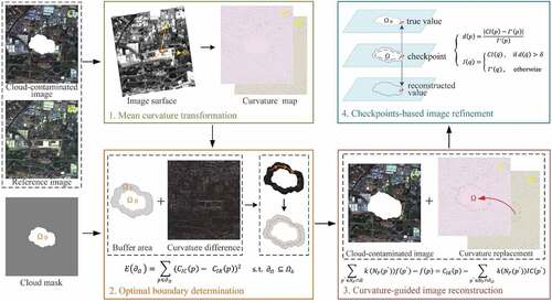
The main idea in this paper is to perform missing information reconstruction in curvature domain rather than in natural domain because the curvature can well reflect the texture information. The flowchart of the proposed method has been illustrated in Figure 1. There are four main steps, including the mean curvature transformation, optimal boundary determination, curvature-guided image reconstruction, and checkpoints-based image refinement. The input data includes the coregistered cloud-contaminated image and reference image, and the cloud mask is also required to determine the area to be restored. The first step is mean curvature transformation, through which the image can be transformed from natural domain to curvature domain, as shown in the green rectangle. The second step is optimal boundary determination. In this step, the curvature differences between two images are calculated and the buffer of cloud coverage area is constructed, then the boundary is optimized within the buffer area to make the boundary pass through these pixels with minimum curvature difference. This step is marked in orange rectangle, in which the optimized boundary is marked with the orange dotted line. The third step is curvature-guided image reconstruction. Based on the optimized boundary for cloud coverage area replacement, the curvature of missing area in cloud-contaminated image is reconstructed with curvature of corresponding area in reference image, then the initial cloud-free image is obtained by inverse curvature transformation of the reconstructed curvature map, which is marked in red rectangle. The last step is checkpoints-based image refinement, which is marked in blue rectangle. In this step, the initial cloud-free result is further refined based on the deviation between the true pixel value and reconstructed pixel value of these checkpoints, and then the final reconstructed image is generated.

Figure 1. The flowchart of the proposed curvature-driven cloud removal method.

2.1. Mean curvature transformation

Curvature indicates the degree of the local bending of a curve or a surface (Liu, Bao, and Peng 2006). Mean curvature is a measure of curvature in three-dimensional Euclidean space that locally describes the curvature of a surface. Figure 2, respectively, shows the curvature of point $P$ in two-dimensional space and three-dimensional space.

Figure 2. The curvature. (a) The curvature in two-dimensional space. (b) The curvature in three-dimensional space.

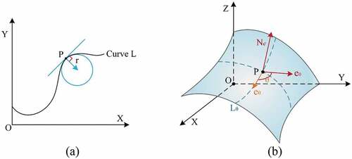
In the geometric sense, the curvature of a curve in two-dimensional space is determined by the radius of the curve’s osculating circle, as shown in Figure 2(a). For the given point $P$, there is a circle tangent to curve $L$ at $P$, and the curvature of point $P$ is $1/r$. When turning to three-dimensional space, the mean curvature at $P$ of the surface is the average of the curvature over all angles (Park et al. 2005). For point $P$ of the surface in Figure 2(b), $N_e$ is the normal of $P$, $e_0$ is assumed to be the starting direction on the tangent plane of $P$, the angle between $e_0$ and $e_{\theta }$ is $\theta$, and $L_{\theta }$ is the curve that go through $P$ in $e_{\theta }.$ Let $c_{\theta }$ be the curvature of curve $L_{\theta }$, then the mean curvature $C$ can be expressed as:

(1) $\begin{array}{c}C=\frac{1}{2\pi }{\int }_0^{2\pi }{c}_{\theta }d\theta \end{array}$(1)

Mean curvature can also be represented by:

(2) $\begin{array}{c}C=\frac{c_{\mathrm{m}\mathrm{a}\mathrm{x}}+c_{\mathrm{m}\mathrm{i}\mathrm{n}}}{2}\end{array}$(2)

Here, $c_{\mathrm{m}\mathrm{a}\mathrm{x}}$ and $c_{\mathrm{m}\mathrm{i}\mathrm{n}}$ are the maximum curvature and minimum curvature, respectively. $c_{\mathrm{m}\mathrm{a}\mathrm{x}}$ and $c_{\mathrm{m}\mathrm{i}\mathrm{n}}$ are also called the two principal curvatures at $P$ of the surface, which can be represented as:

(3) $c_{\mathrm{m}\mathrm{a}\mathrm{x}}=max\left\{c_{\theta }\left(\theta \right)\right\},\hspace{0.17em}\theta \hspace{0.17em}\in \left[0,2\pi \right]$(3)

(4) $c_{\mathrm{m}\mathrm{i}\mathrm{n}}=min\left\{c_{\theta }\left(\theta \right)\right\},\hspace{0.17em}\theta \hspace{0.17em}\in \left[0,2\pi \right]$(4)

Since digital images are usually regularly sampled and composed of discrete pixels, “image surface” is used to refer this type of surfaces (Zhu and Chan 2012). For example, the image surface of image $I$ is represented by $\left(x,y,I\left(x,y\right)\right)$, where $I\left(x,y\right)$ denotes the pixel value of the image at pixel $\left(x,y\right).$ Typically, for image $I$, the mean curvature is computed by (Gong and Goksel 2019):

(5) $C\left(I\right)=\frac{1}{2}\mathrm{\Delta }\hspace{0.17em}\frac{\mathrm{\nabla }I}{{∥\mathrm{\nabla }I∥}_2}$(5)

where $\mathrm{\nabla }$ is gradient operator, $\mathrm{\Delta }$ is divergence operator. Therefore, it can also be expressed as:

(6) $C\left(I\right)=\frac{\left(1+I_x^2\right)I_{yy}+2I_x{I}_y{I}_{xy}+\left(1+I_y^2\right)I_{xx}}{2{\left(1+I_x^2+I_y^2\right)}^{\frac{3}{2}}}$(6)

This is a traditional way for curvature calculation, which involves the second-order derivatives. In order to simply the calculation, Gong and Sbalzarini (2017) proposed a simple convolution operation for mean curvature estimation, which can be expressed as:

(7) $\begin{array}{c}C\left(I\right)=k_m\otimes I\end{array}$(7)

where $k_m$ denotes the mean curvature operator, and ⊗ denotes the convolution operation.

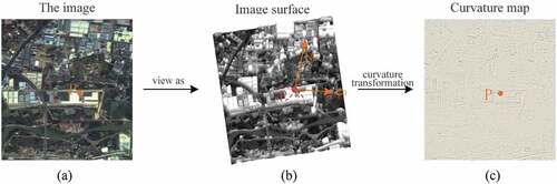
In Equation (7)(7) $\begin{array}{c}C\left(I\right)=k_m\otimes I\end{array}$(7) , the convolution operation is performed for each pixel of the image, whether it is a cloud pixel or a cloud-free pixel, to calculate the curvature value of the pixel according to the gray value of its neighboring pixels. Afterward, the mean curvature of image I is obtained. Here, “curvature map” is used to refer the curvature transformation result of an image, and the process of obtaining the curvature map from an image is the transformation from natural domain to curvature domain, as shown in Figure 3. Different from natural domain, the object to be processed in curvature domain is the curvature of each pixel.

Figure 3. The transformation from natural domain to curvature domain. (a) Image in natural domain. (b) Image surface. (c) The curvature map of (a) in curvature domain.

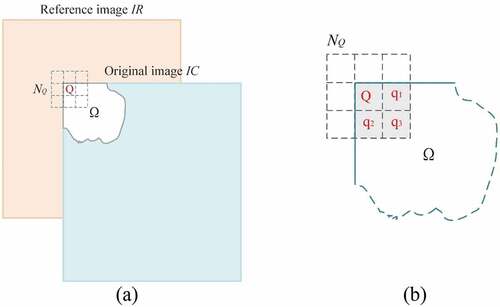
2.2. Optimal boundary determination

In the process of curvature reconstruction, the result will appear inconsistent and discontinuous if the curvature of cloud-contaminated image is quite different from that of reference image at the cloud boundary. Therefore, in order to ensure the continuity of reconstructed image, the boundary for cloud coverage area replacement is optimized before curvature reconstruction to make the boundary pass through the pixels with minimum curvature difference.

In order to determine the optimal boundary with the minimum curvature cost, a buffer should be constructed first, then the next step is to calculate the curvatures of images according to:

(8) $\begin{array}{c}{C}_{IC}=k_m\otimes IC\end{array}$(8)

(9) $\begin{array}{c}{C}_{IR}=k_m\otimes IR\end{array}$(9)

where $IC$ and $IR$, respectively, represent the cloud-contaminated image and reference image, and $C_{IC}$ represents the curvature map of $IC$.

Then the boundary energy function needs to be defined to calculate the curvature cost of different boundaries. Supposing that ${\partial }_{\Omega }$ represents the optimized boundary, and $p$ represents the pixel on ${\partial }_{\Omega }$, the boundary energy function can be formulated as follows:

(10) $E\left({\partial }_{\Omega }\right)=\sum _{p\in {\partial }_{\Omega }}{\left(C_{IC}\left(p\right)-C_{IR}\left(p\right)\right)}^2,s.t.\partial \Omega \subseteq {\Omega }_b$(10)

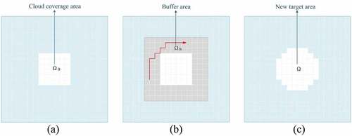
The Equation (10)(10) $E\left({\partial }_{\Omega }\right)=\sum _{p\in {\partial }_{\Omega }}{\left(C_{IC}\left(p\right)-C_{IR}\left(p\right)\right)}^2,s.t.\partial \Omega \subseteq {\Omega }_b$(10) can be minimized based on a shortest closed-path algorithm proposed by Jia et al. (2006). According to the solution of the boundary energy function above, the optimized boundary is calculated and the new target area to be replaced is determined. There is an illustration shown in Figure 4 for explanation. The cloud coverage area, the buffer area, and the new target area after boundary optimization are, respectively, shown in Figure 4(a–c).

Figure 4. The optimal boundary determination. (a) The cloud coverage area. (b) The buffer area. (c) New target area after boundary optimization.

2.3. Curvature-guided image reconstruction

Base on the optimized boundary for cloud coverage area replacement determined in the previous step, the curvature-guided image reconstruction is to recover the curvature of cloud coverage area in cloud-contaminated image with the curvature of reference image, and then inversely transform the reconstructed curvature map back to natural domain to generate the initial cloud-free result. The reconstructed curvature map of cloud-contaminated image $IC$ can be expressed as:

(11) $\begin{array}{c}{C}_{IC}^{\ast }\left(p\right)=\left\{\begin{array}{c}{C}_{IC}\left(p\right),p\in \bar{\mathrm{\Omega }}\\ C_{IR}\left(p\right),p\in \mathrm{\Omega }\end{array}\right.\end{array}$(11)

where $C_{IC}^{\ast }\left(p\right)$ represents the curvature of pixel $p$ in the reconstructed curvature map $C_{IC}^{\ast }$, $\mathrm{\Omega }$ is the new target area after boundary optimization, and $\bar{\mathrm{\Omega }}$ is the area outside $\mathrm{\Omega }$.

Inspired by the Poisson editing algorithm (Perez, Gangnet, and Blake 2003), the inverse transformation process in this paper is formulated as a global optimization problem with Dirichlet boundary condition. Let $I^{\ast }$ be the reconstructed cloud-free image, then this problem can be naturally discretized into:

(12) $\begin{array}{rl}& \underset{I^{\ast }{|}_{\mathrm{\Omega }}}{min}\sum _{p\in \mathrm{\Omega }}{\left(C_{I\ast }\left(p\right)-C_{IC}^{\ast }\left(p\right)\right)}^2,\\ & \mathrm{w}\mathrm{i}\mathrm{t}\mathrm{h}{I}^{\ast }\left(q\right)=IC\left(q\right),forallq\in \mathrm{\partial }\mathrm{\Omega }\end{array}$(12)

According to Equation (7)(7) $\begin{array}{c}C\left(I\right)=k_m\otimes I\end{array}$(7) , the curvature of each pixel $p$ in the discrete image is determined by the pixel of its 8-connected neighbors. Supposing the set of 8-connected neighbors of $p$ is $N_P$, the pixel in $N_P$ is $p{ }^{\mathrm{\prime }}$, then the solution of Equation (12)(12) $\begin{array}{rl}& \underset{I^{\ast }{|}_{\mathrm{\Omega }}}{min}\sum _{p\in \mathrm{\Omega }}{\left(C_{I\ast }\left(p\right)-C_{IC}^{\ast }\left(p\right)\right)}^2,\\ & \mathrm{w}\mathrm{i}\mathrm{t}\mathrm{h}{I}^{\ast }\left(q\right)=IC\left(q\right),forallq\in \mathrm{\partial }\mathrm{\Omega }\end{array}$(12) satisfies the following linear equations:

(13) $\begin{array}{rl}& \sum _{p\mathrm{\prime }\in N_P\cap {}_{\mathrm{\Omega }}}k\left(N_P\left(p^{\mathrm{\prime }}\right)\right)I^{\ast }\left(p^{\mathrm{\prime }}\right)-I^{\ast }\left(p\right)=C_{IC}^{\ast }\left(p\right)\\ & -\sum _{p\mathrm{\prime }\in N_P\cap {\mathrm{\partial }}_{\mathrm{\Omega }}}k\left(N_P\left(p^{\mathrm{\prime }}\right)\right)IC\left(p^{\mathrm{\prime }}\right),p\in \mathrm{\Omega }\end{array}$(13)

Here, $N_P\left(p{ }^{\mathrm{\prime }}\right)$ represents the position of $p{ }^{\mathrm{\prime }}$ relative to $p$ in the 8-connected neighbors, and $k\left(N_P\left(p{ }^{\mathrm{\prime }}\right)\right)$ represents the coefficient of $N_P\left(p{ }^{\mathrm{\prime }}\right)$ in the curvature convolution operator $k_m$.

(14) $\begin{array}{rl}& N_P\left(p^{\mathrm{\prime }}\right)=\left\{\left(-1,-1\right),\left(-1,0\right),\left(-1,1\right),\left(0,-1\right)\right.,\\ & \left.\left(0,1\right),\left(1,-1\right),\left(1,0\right),\left(1,1\right)\right\}\end{array}$(14)

(15) $\begin{array}{c}k\left(N_P\left(p{ }^{\mathrm{\prime }}\right)\right)=\left\{-\frac{1}{16},\frac{5}{16},-\frac{1}{16},\frac{5}{16},\frac{5}{16},-\frac{1}{16},\frac{5}{16},-\frac{1}{16}\right\}\end{array}$(15)

Equation (13)(13) $\begin{array}{rl}& \sum _{p\mathrm{\prime }\in N_P\cap {}_{\mathrm{\Omega }}}k\left(N_P\left(p^{\mathrm{\prime }}\right)\right)I^{\ast }\left(p^{\mathrm{\prime }}\right)-I^{\ast }\left(p\right)=C_{IC}^{\ast }\left(p\right)\\ & -\sum _{p\mathrm{\prime }\in N_P\cap {\mathrm{\partial }}_{\mathrm{\Omega }}}k\left(N_P\left(p^{\mathrm{\prime }}\right)\right)IC\left(p^{\mathrm{\prime }}\right),p\in \mathrm{\Omega }\end{array}$(13) contains the case where the pixel $p$ is at the boundary of $\mathrm{\Omega }$, that is $N_P\cap {\partial }_{\Omega }\ne \varphi .$. When $N_P\subseteq \Omega$, that is, $N_P\cap {\partial }_{\Omega }=\varnothing$, there is no boundary term on the right of Equation (13)(13) $\begin{array}{rl}& \sum _{p\mathrm{\prime }\in N_P\cap {}_{\mathrm{\Omega }}}k\left(N_P\left(p^{\mathrm{\prime }}\right)\right)I^{\ast }\left(p^{\mathrm{\prime }}\right)-I^{\ast }\left(p\right)=C_{IC}^{\ast }\left(p\right)\\ & -\sum _{p\mathrm{\prime }\in N_P\cap {\mathrm{\partial }}_{\mathrm{\Omega }}}k\left(N_P\left(p^{\mathrm{\prime }}\right)\right)IC\left(p^{\mathrm{\prime }}\right),p\in \mathrm{\Omega }\end{array}$(13) , which can be expressed as:

(16) $\sum _{p\prime \in N_P}k\left(N_P\left(p^{\prime }\right)\right)I^{*}\left(p\prime \right)-I^{*}\left(p\right)=C_{IC}^{*}\left(p\right),N_P\in \Omega$(16)

Especially, when the cloud coverage area locates at the corner of image, the curvature equation of the pixel at the boundary can be calculated according to:

(17) $\begin{array}{rl}& \sum _{p^{\mathrm{\prime }}\in N_P\cap \mathrm{\Omega }}k\left(N_P\left(p^{\mathrm{\prime }}\right)\right)I^{\ast }\left(p^{\mathrm{\prime }}\right)-\left(\sum _{p^{\mathrm{\prime }}\in N_P\cap \mathrm{\Omega }}k\left(N_P\left(p^{\mathrm{\prime }}\right)\right)\right)\\ & I^{\ast }\left(p\right)=C_{IC}^{\ast }\left(p\right),p\in {\mathrm{\partial }}_{IC}\cap {\mathrm{\partial }}_{\mathrm{\Omega }}\end{array}$(17)

Figure 5 shows the above special case. Figure 5(a) shows the relative position of cloud-contaminated image and reference image, and Figure 5(b) shows the detail of cloud coverage area. There is a pixel $Q$ located at the image boundary ${\partial }_{IC}$, and its 8-connected neighbors $N_Q$ only contain $q_1$, $q_2$ and $q_3$. Therefore, the curvature equation of $Q$ is expressed as:

Figure 5. The case when the cloud coverage area is in the corner of the image. (a) The relative position of images. (b) The details of the cloud coverage area.

(18) $\sum _{i=1}^3\left(k\left(N_Q\left(q_i\right)\right)\cdot I^{*}\left(q_i\right)\right)-\left(\sum _{i=1}^{3}k\left(N_Q\left(q_i\right)\right)\right)I^{*}\left(Q\right)=C_{IC}^{*}\left(Q\right)$(18)

After constructing the curvature equations of all pixels, the whole process is mathematically formulated as a positive definite linear equations system, and the coefficient matrix is sparse and symmetrical, which can be calculated by iterative solver. Thus, the initial cloud-free result is reconstructed.

2.4. Checkpoints-based image refinement

Checkpoints in this paper refer to these newly added pixels of the new target area after boundary optimization compared with the cloud coverage area. The checkpoints-based image refinement is to further refine initial cloud-free result $I^{\ast }$ based on the deviation between true value and reconstructed value of these checkpoints. After $I^{\ast }$ is reconstructed by solving the curvature equations above, for the checkpoints in $\mathrm{\Omega }$, there are both the true value from cloud-contaminated image $IC$ and reconstructed value from the initial cloud-free result $I^{\ast }$, as shown in Figure 6.

Figure 6. The deviation between true value and reconstructed value of these checkpoints.

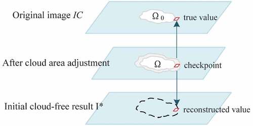
Considering the possible inconsistency of radiometric differences between various ground features, there may be still some differences between these checkpoints in $I^{\ast }$ and $IC$. Therefore, the initial cloud-free result $I^{\ast }$ is further refined based on these checkpoints. First, for the checkpoint $p\in \mathrm{\Omega }-{\mathrm{\Omega }}_0$, that is, $p\in \mathrm{\Omega }$ and $p\notin {\mathrm{\Omega }}_0$, the deviation $d$ can be calculated by:

(19) $\begin{array}{c}d\left(p\right)=\frac{\left|IC\left(p\right)-I^{\ast }\left(p\right)\right|}{I^{\ast }\left(p\right)}\end{array}$(19)

Let $I$ be the final reconstructed image, then each pixel $q\in \mathrm{\Omega }$ in $I$ will be modified according to:

(20) $\begin{array}{c}I\left(q\right)=\left\{\begin{array}{c}IC\left(\bar{q}\right),ifd\left(q\right)>\delta \\ \\ I^{\ast }\left(q\right),otherwise\end{array}\right.\end{array}$(20)

where $\delta$ is defined as $2{\sigma }_{d\left(p\right)}$, and ${\sigma }_{d\left(p\right)}$ is the standard deviation, which is used to identify changing pixels. And $\bar{q}$ represents the corresponding pixel of $q$ in $\mathrm{\Omega }-{\mathrm{\Omega }}_0$, which is determined by:

(21) $\begin{array}{c}\bar{q}=arg\underset{q^{\prime }\in {\mathrm{\Omega }}_q}{max}S\left(N_q,N_{q^{\prime }}\right)\end{array}$(21)

where $S\left(N_q,N_{q^{\prime }}\right)$ represents the correlation coefficient of $N_q$ and $N_{q^{\prime }}$, and ${\mathrm{\Omega }}_q$ represents the set related to the current pixel $q$, which is defined as:

(22) $\begin{array}{c}{\mathrm{\Omega }}_q=\left\{q^{\prime }|I^{\ast }\left(q^{\prime }\right)=I^{\ast }\left(q\right),q^{\prime }\in \mathrm{\Omega }-{\mathrm{\Omega }}_0\right\}\end{array}$(22)

Finally, the reconstructed result $I$ is obtained.

3. Experimental results and discussion

Both simulated experiments and real data experiments are conducted to verify the performance of the proposed method. The results of the proposed method are compared with those of other information reconstruction methods including Poisson blending method, Poisson blending with boundary optimization, the Weighted Linear Regression method (WLR), and the Progressive Spatio-temporal Cloud Removal method (PSTCR). The Poisson blending method (Perez, Gangnet, and Blake 2003) is a classic method and has been widely used in image inpainting. The Poisson blending with boundary optimization is improved on the basis of the Poisson blending method, which first optimizes the boundary for cloud coverage area replacement and then performs Poisson blending process (Lai and Lin 2012). WLR (Zeng, Shen, and Zhang 2013) is carried out pixel by pixel by establishing a regression model between the corresponding pixels in cloud-contaminated image and reference image. PSTCR (Zhang et al. 2020) is a novel cloud removal method for multitemporal images based on deep learning, and this paper downloaded the trained framework from https://github.com/WHUQZhang/PSTCR for experiments.

3.1. Simulated experiments

Three sections are included in simulated experiments. The first section is to evaluate the effectiveness of the proposed method, and two groups of images with different resolutions are used as experimental data. The second section is to analyze the sensitivity of the proposed method to the boundary optimization procedure, and the third section is to evaluate the impacts of different cloud coverage on the performance of the proposed method. In this paper, simulated data is generated from the original cloud-free image. Since the original image is reasonable ground truth, the reconstructed result can be evaluated from both visual and quantitative aspects.

There are five indexes used for quantitative analyses, including the Mean Structural Similarity Index Metric (MSSIM) (Zhou and Bovik 2002), the Multi-scale Structural Similarity Index Metric (MS-SSIM) (Wang, Simoncelli, and Bovik 2003), the Peak Signal-to-noise Ratio (PSNR), the Correlation Coefficient (CC), and the Cross Entropy (CE). SSIM is an index that integrates the three aspects of luminance, contrast, and structure to assess similarity between images, and MSSIM applies SSIM to local regions using a sliding window approach. Let $I^0$ be the original clear image, $I$ be the reconstructed result, $L$, $C$ and $S$ represent the luminance, contrast, and structure components, respectively. Then MSSIM can be calculated according to:

(23) $\begin{array}{c}L\left(I,I^0\right)=\frac{2u_I{u}_{I^0}+c_1}{u_I^2+u_{I^0}^2+c_1}\end{array}$(23)

(24) $\begin{array}{c}C\left(I,I^0\right)=\frac{2{\sigma }_I{\sigma }_{I^0}+c_2}{{\sigma }_I^2+{\sigma }_{I^0}^2+c_2}\end{array}$(24)

(25) $\begin{array}{c}S\left(I,I^0\right)=\frac{{\sigma }_{I,I^0}+c_3}{{\sigma }_I{\sigma }_{I^0}+c_3}\end{array}$(25)

(26) $\begin{array}{rl}& MSSIM\left(I,I^0\right)=\frac{1}{B}\sum _{b=1}^B\mathrm{S}\mathrm{S}\mathrm{I}\mathrm{M}\left(I_b,{I^0}_b\right)\\ & =\frac{1}{B}\sum _{b=1}^{B}L\left(I_b,{I^0}_b\right)C\left(I_b,{I^0}_b\right)S\left(I_b,{I^0}_b\right)\end{array}$(26)

where $B$ is the total number of sliding windows$,$ $u$, ${\sigma }_{I,I^0}$ and ${\sigma }^2$ represent the mean value, the covariance, the variance, respectively. $c_1$, $c_2$, and $c_3$ are three small constants used to avoid unstable result when denominator is close to 0.

MS-SSIM is the extension of SSIM in multi-scale space, which is computed by iteratively downsampling images by a factor of 2 using:

(27) $\begin{array}{rl}& MS-SSIM\left(I,I^0\right)={\left[L_M\left(I,I^0\right)\right]}^{{\alpha }_M}\\ & \cdot \prod _{m=1}^M{\left[C_m\left(I,I^0\right)\right]}^{{\beta }_m}{\left[S_m\left(I,I^0\right)\right]}^{{\gamma }_m}\end{array}$(27)

where $M$ is the highest downsampling scale, ${\alpha }_M$, ${\beta }_m$, and ${\gamma }_m$ are constants used to adjust the proportion of different components. Usually, $M=5$, ${\alpha }_5=0.1333$, $\beta =\gamma =\left[0.0448,0.2856,0.3001,0.2363,0.1333\right]$.

PSNR is an index to evaluate the degree of image distortion, which is defined as:

(28) $\begin{array}{c}PSNR\left(I,I^0\right)=20\ast \mathrm{l}\mathrm{o}{\mathrm{g}}_{10}\left(\frac{\mathrm{M}\mathrm{A}{\mathrm{X}}_{I,I^0}}{\sqrt{\mathrm{M}\mathrm{S}\mathrm{E}\left(I,I^0\right)}}\right)\end{array}$(28)

(29) $\begin{array}{c}MSE\left(I,I^0\right)=\frac{1}{hw}\sum _{i=1}^h\sum _{j=1}^w{\left[I\left(i,j\right)-I^0\left(i,j\right)\right]}^2\end{array}$(29)

where $\mathrm{M}\mathrm{A}{\mathrm{X}}_{I,I^0}$ is the maximum pixel value of images, $I\left(i,j\right)$ represents the pixel value at $\left(i,j\right)$, $h$ and $w$ represent the height and width of image.

CC can be used to measure the similarity of two images, which is calculated according to Equation (24)(24) $\begin{array}{c}C\left(I,I^0\right)=\frac{2{\sigma }_I{\sigma }_{I^0}+c_2}{{\sigma }_I^2+{\sigma }_{I^0}^2+c_2}\end{array}$(24) and $c_3=0$. The higher the values of the above four indexes, the better the consistency between the reconstructed result and the original clear image. CE is also a common index to measure the differences between images. A lower CE indicates a better result, which is given by

(30) $CE\left(I,I^0\right)=\sum _{k=1}^{\text{MAX}-1}{I}^0\left(k\right){\text{log}}_2\left(\frac{I^0\left(k\right)}{I\left(k\right)}\right)$(30)

where $I^0\left(k\right)$ and $I\left(k\right)$, respectively, represent the probability of pixel value $k$ in $I^0$ and $I$.

3.1.1 Effectiveness of the proposed method

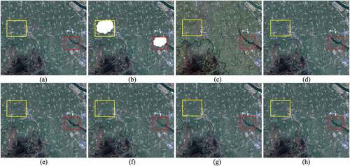
The first group experiment was conducted on GF1 PMS images with the resolution of 8 m, and three bands of blue, green, and red bands were used for further test. The experimental data is shown in Figure 7. Figure 7(a) is original cloud-free image, Figure 7(b) is the image with two simulated clouds of different sizes, and Figure 7(c) is reference cloud-free image. Figure 7(d–h) show the cloud removal results generated by Poisson blending method, Poisson blending with boundary optimization, WLR, PSTCR, and the proposed method, respectively. There are significant radiometric differences between the buildings in original image and reference image, and the color of buildings in reconstructed area of Figure 7(d–f) is a little abnormal, especially in the yellow rectangle area, which is inconsistent with the color of buildings in other areas.

Figure 7. GF1 PMS images for simulated experiment. (a) Original cloud-free image. (b) Simulated cloud image. (c) Reference image. (d) Result of Poisson blending method. (e) Result of Poisson blending with boundary optimization. (f) Result of WLR. (g) Result of PSTCR. (h) Result of the proposed method.

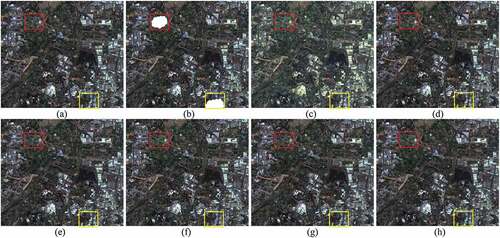
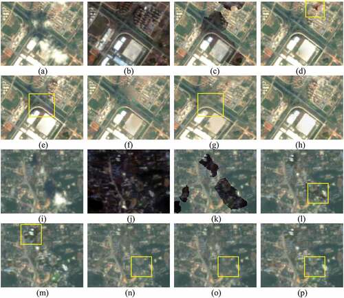
The zoomed details of Figure 7 are shown in Figure 8. Figures 8(a–h) are the details of the red rectangle area in Figure 7(a–h), respectively. Figure 8(i–p) are the details of the yellow rectangle area in Figure 7(a–h), respectively. Generally, the color of most ground objects in cloud removal results is more consistent with original image than reference image, such as the road in Figure 8(a–h) and the land in Figure 8(i–p). However, in Figure 8(d), there is still a slight discontinuity inside the building in the yellow rectangle, and the part of the building outside the area is brighter than the reconstructed area. After boundary optimization, the radiometric continuity of Figure 8(e) is better, but the color of the building is darker compared to original image shown in Figure 8(a). Since WLR is performed pixel by pixel, the spatial continuity in Figure 8(f) may be slightly poor. The color in Figure 8(g–h) are more fidelity, such as the color of buildings in the yellow rectangles. However, slight discontinuity appears in the yellow circle area in Figure 8(g). The situation is similar in Figure 8(i–p), the overall color of Figure 8(p) is closer to the original image than Figure 8(o), especially in the yellow rectangle area, and the color of building is also well restored without discontinuity. In addition to qualitative visual analyses, quantitative analyses have also been conducted, as shown in Table 1, in which symbol ↑ means the higher the index, the better the result, and symbol ↓ means that the lower the index, the better the result. The proposed method achieves higher MSSIM, MS-SSIM and CC, indicating that the reconstructed result is more similar with original result in luminance, contrast, and structure. The higher PSNR and lower CE also show that the higher reconstruction accuracy of the proposed method when compared with other four methods.

Figure 8. The zoomed details of Figure 7. (a)–(h) are the details of the red rectangle area in Figure 7(a–h). (i)–(p) are the details of the yellow rectangle area in Figure 7(a–h).

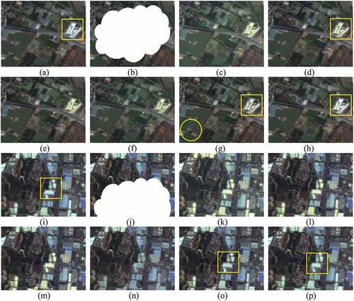
Table 1. The MSSIM, MS-SSIM, PSNR, CC, and CE values of the experimental results in Figure 7.

	MSSIM$\uparrow$	MS-SSIM$\uparrow$	PSNR$\uparrow$	CC$\uparrow$	CE $\downarrow$
Poisson blending method	0.8594	0.9081	27.53	0.9475	0.1044
Poisson blending with boundary optimization	0.8648	0.9099	27.83	0.9472	0.0792
Weighted linear regression method	0.8539	0.9107	27.56	0.9496	0.1149
PSTCR method	0.8750	0.9133	28.49	0.9539	0.0773
The proposed curvature-based method	0.9046	0.9131	31.22	0.9553	0.0331

The second group experiment was conducted on GF1 WFV images with a resolution of 16 m. The experimental data are shown in Figure 9. Figure 9(a) is original cloud-free image, Figure 9(b) is the image with two simulated clouds. Figure 9(c) is reference- image. The cloud removal results of Poisson blending method, Poisson blending with boundary optimization, WLR, PSTCR, and the proposed method are shown in Figure 9(d–h), respectively. Colors of river and land in Figure 9(b) are quite different from that in Figure 9(c). Although these differences are greatly reduced in Figure 9(d–h), there are still some color inconsistencies in rivers in Figure 9(d,f).

Figure 9. GF1 WFV images for simulated experiment. (a) Original cloud-free image. (b) Simulated cloud image. (c) Reference image. (d) Result of Poisson blending method. (e) Result of Poisson blending with boundary optimization. (f) Result of WLR. (g) Result of PSTCR. (h) Result of the proposed method.

Figure 10 shows the zoomed details of Figure 9. Figure 10(a–h) are the details of the red rectangle area in Figure 9(a–h), respectively. Figure 10(i–p) are the details of the yellow rectangle area in Figure 9(a–h), respectively. Obviously, colors of land in Figure 10(d–f) are much closer to that in Figure 10(a) than in Figure 10(c), but there are still some differences in the color of the river. In the reconstructed area of Figure 10(d–e), the river appears darker than that in the original image. In Figure 10(f), there is also something wrong with the color of the river and its spatial continuity is slightly poor. In contrast, the reconstructed results shown in Figure 10(g–h) are much closer to Figure 10(a), and the color of the river is also well restored. Compared to the original image shown in Figure 10(i), there are still some color differences in Figure 10(l,m), mainly reflected by the color of the river. The spatial discontinuity problem also occurs in the yellow rectangle area in Figure 10(n). In Figure 10(o), some details in the yellow rectangle area are blurred. Figure 10(p) is more similar with original image and shows a higher reconstruction accuracy. Table 2 shows the quantitative analyses of these results, where the higher MSSIM, MS-SSIM, CC, PSNR, and the lower CE also indicate the strength of the proposed method.

Figure 10. The zoomed details of Figure 9. (a)–(h) are the details of the red rectangle area in Figure 9(a–h). (i)–(p) are the details of the yellow rectangle area in Figure 9(a–h).

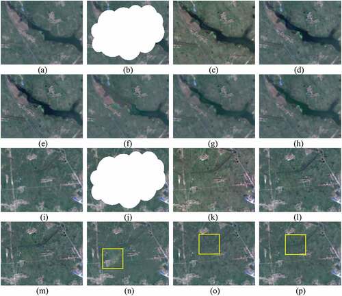
Table 2. The MSSIM, MS-SSIM, PSNR, CC, and CE values of the experimental results in Figure 9.

	MSSIM$\uparrow$	MS-SSIM$\uparrow$	PSNR$\uparrow$	CC$\uparrow$	CE $\downarrow$
Poisson blending method	0.8250	0.8696	27.01	0.8621	0.1093
Poisson blending with boundary optimization	0.8257	0.8703	27.24	0.8673	0.1292
Weighted linear regression method	0.8362	0.8831	27.79	0.8475	0.1811
PSTCR method	0.8453	0.8756	27.73	0.8769	0.0830
The proposed curvature-based method	0.8491	0.8835	28.36	0.8737	0.0229

3.1.2 Sensitivity to the boundary optimization procedure

Two GF1 PMS images with 8 m resolution were used as experimental data in this section, and Figure 11(a) shows original cloud-free image and reference image. Different sizes of the buffer areas, which determine the searching range of the optimal boundary detection, were set in this experiment to evaluate the sensitivity of the proposed method to the boundary optimization procedure. Figure 11(b) shows the simulated cloud-contaminated image and the cloud removal result without boundary optimization, that is, the size of buffer area is 0. Figure 11(c–f) show the experimental data of different sizes of buffer areas, including the optimized boundary results and the cloud removal results. The sizes of buffer areas in Figure 11(c–f) are 5 pixels, 10 pixels, 20 pixels, 30 pixels, respectively.

Figure 11. Sensitivity of the proposed method to boundary optimization procedure. (a) includes original image and reference image. (b)–(f) are the experimental data of different sizes of buffer areas, including the optimized boundary results and the cloud removal results. The sizes of buffer areas in (b)-(f) are 0 pixels, 5 pixels, 10 pixels, 20 pixels, 30 pixels, respectively.

Figure 12 shows the zoomed details of the marked rectangle areas in Figure11. Figure 12(a–f) are the details of the red rectangle areas in Figure 11(a–f), respectively. Figure 12(g–l) are the details of the yellow rectangle areas in Figure 11(a–f), respectively. The yellow lines near the clouds in Figure 12 indicate the optimized boundary. In Figure 12(a), the ship is the object that has changed between two images. When the cloud boundary crosses through the changed area, the whole object in the restored image may be cut into incomplete ones, as shown in Figure 12(b). Figure 12(c) shows the results after boundary optimization, and the size of buffer area is 5 pixels. Since the size of buffer area is smaller than that of the ship, the optimized boundary cannot bypass the ship. However, in Figure 12(d), the incomplete ship disappears when the size of buffer area is 10 pixels. When the sizes of buffer areas are 20 pixels and 30 pixels, there is no obvious difference in the cloud removal results, as shown in Figure 12(e–f). Due to the differences between original image and reference image in the red rectangle area of Figure 14(g), spatial discontinuities appear in in Figure 14(h), which is the result without boundary optimization. This problem is also present in Figure 14(i), since the optimized boundary is still inside the abnormal area. When the size of buffer area is 10 pixels or larger, the spatial discontinuities are almost invisible and the results are more natural, as shown in Figure 14(j–l).

Figure 12. The zoomed details of Figure 11(a–f) are the details of the red rectangle areas in Figure 11(a–f). (g)–(l) are the details of the yellow rectangle areas in Figure 11(a)–(f).

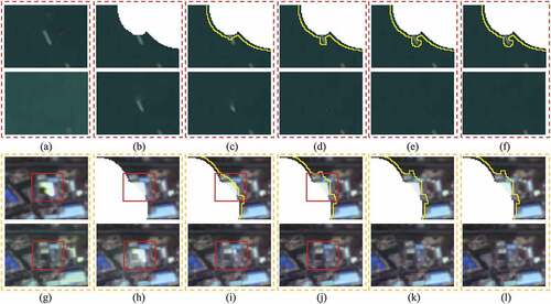
In the quantitative analysis, MSSIM, MS-SSIM, PSNR, CC and CE values are calculated to evaluate the cloud removal results of different buffer areas. Furthermore, the running time is also counted to measure the efficiency. The statistical results are shown in Table 3. The result after boundary optimization with 5-pixel buffer area shows a slightly advantage over the result without boundary optimization, and the differences between these metrics are small. When the size of buffer area is 10 pixels, the metrics do not continue to improve except for CE, and the MSSIM and MS-SSIM even decrease a little compared to the result without boundary optimization. This is because in the boundary optimization process, in order to prevent the object from being cut incompletely and achieve better visual effect, some ground features in the original image may be changed, which reduces the reconstruction accuracy. For example, the incomplete ship in Figure 12(d) is removed compared with the result in Figure 12(b), and the abnormal bright area in Figure 12(h) is replaced with some buildings from reference image, as shown in the red rectangles in Figure 12(j). When the size of buffer area increases, the searching range of the optimal boundary detection is larger, and the algorithm takes longer time. However, the reconstructed result does not change as the buffer area increases when the size of buffer area is larger than 20 pixels, and the results of 10-pixel buffer area and 20-pixel buffer area differ very little in both qualitative and quantitative term. This is because in the 8 m resolution images used in this experiment, most of the ground features are within 80 m, that is, within 10 pixels. Therefore, the boundary optimization procedure is effective with about 10-pixel buffer area in this experiment. This also suggests that the size of buffer area should be determined according to the image resolution. Furthermore, to ensure the effectiveness of the method, a minimum size of 5 pixels is recommended.

Table 3. Quantitative analyses of the experimental results in Figure 11.

Buffer area/pixels	Time/s	MSSIM$\uparrow$	MS-SSIM$\uparrow$	PSNR$\uparrow$	CC$\uparrow$	CE $\downarrow$
0	10.24	0.8613	0.9183	26.61	0.9174	0.1170
5	28.11	0.8617	0.9205	27.31	0.9259	0.1135
10	30.52	0.8612	0.9175	27.01	0.9215	0.0895
20	32.02	0.8612	0.9174	27.01	0.9215	0.0887
30	33.94	0.8612	0.9174	27.01	0.9215	0.0887

3.1.3 Impacts of different cloud coverage on method performance

In order to analyze the influence of different cloud coverage on the performance of the proposed method, this experiment was conducted on GF1 WFV multispectral images with different cloud coverage, including thick and thin clouds, and covering about 20% to 90%. The thin clouds in the section are generated from Photoshop according to https://helpx.adobe.com/photoshop-elements/using/render-filters.html. The experimental data is composed of 4 bands: red, green, blue and Near Infrared (NIR). With false color composition, the original cloud-free image and reference image are, respectively, shown in Figure 13(a,b), the simulated images and the cloud removal results with different cloud sizes are shown in Figure 13(c–j). The percentages of cloud coverage are 19.64% in Figure 13(c), 30.13% in Figure 13(d), 40.05% in Figure 13(e), 50.24% in Figure 13(f), 59.79% in Figure 13(g), 70.14% in Figure 13(h), 79.75% in Figure 13(i), 90.26% in Figure 13(j), respectively. And Figure 13(c,e,g,i) are simulated with thick clouds, Figure 13(d,f,h,j) are simulated with thin clouds.

Figure 13. Experimental data with different cloud coverage. (a) Original cloud-free image. (b) Reference image. (c)-(j) Simulated images and cloud removal results of the proposed method on different cloud coverage. The percentages of cloud coverage in (c)-(j) are, respectively, 19.64%, 30.13%, 40.05%, 50.24%, 59.79%, 70.14%, 79.75%, 90.26%. (c), (e), (g) and (i) are simulated with thick clouds, and (d), (f), (h) and (j) are simulated with thin clouds.

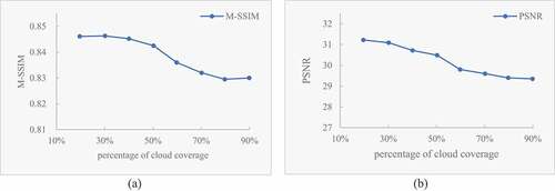
In Figure 13, the proposed method obtains satisfactory cloud removal results not only for thick clouds but also for thin clouds. The proposed method utilizes the auxiliary information from reference image to restore the regions identified as clouds in the cloud detection result, so these thin clouds can also be reconstructed if they are successfully detected. According to the zoomed results of the yellow rectangle areas in Figure 13, the proposed method can generate cloud-free images under different cloud coverage conditions, even if the percentage of cloud coverage in the image reaches 90%. In addition, the M-SSIM and PSNR indexes are also calculated for quantitative analyses in this experiment, as shown in Figure 14. Although the M-SSIM and PSNR values decline as the cloud size increases, the decreasing rate are within 2% (M-SSIM) and 6% (PSNR). When the cloud coverage is close to 80%, the results of the two indexes tend to be stable and remain around 0.83 (M-SSIM) and 29 (PSNR), respectively. Thus, the proposed method is proved to be effective for images with different cloud coverage.

Figure 14. The M-SSIM and PSNR values of the results with different simulated cloud sizes.

3.2. Real data experiments

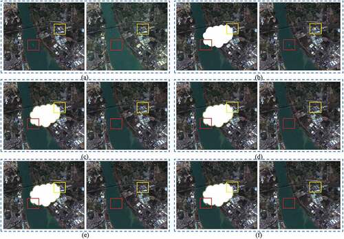
In real data experiments, three groups of images including GF1 PMS images with a resolution of 8 m, GF1 WFV images with a resolution of 16 m, and Sentinel-2A multispectral images with a resolution of 20 m were used. The cloud masks of cloud-contaminated images in real data experiments were obtained from (Dong et al. 2019). The first group of experimental data is shown in Figure 15. Figure 15(a, b) show the cloud-contaminated image and reference image, respectively. Figure 15(c) is the cloud removal result by direct replacement, that is, the cloud coverage area in original cloud-contaminated image is replaced by the corresponding clear area in reference image. The cloud removal results reconstructed by Poisson blending method, Poisson blending with boundary optimization, WLR, PSTCR, and the proposed method are, respectively, shown in Figure 15(d–h). Due to the significant radiometric differences between images, there is an obvious radiometric discontinuity in the cloud removal result of simple replacement, as shown in Figure 15(c). Some details of the marked rectangle areas in Figure 15 are shown in Figure 16.

Figure 15. GF1 PMS images for real data experiment. (a) Cloud-contaminated image. (b) Reference image. (c) Result of direct replacement. (d) Result of Poisson blending method. (e) Result of Poisson blending with boundary optimization. (f) Result of WLR. (g) Result of PSTCR. (h) Result of the proposed method.

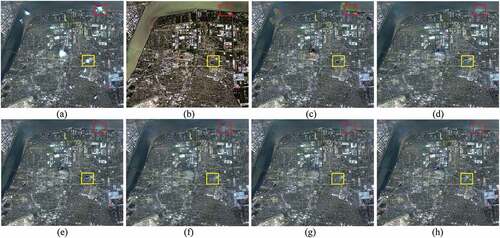
Figure 16. The zoomed details of Figure 15. (a)–(h) are the details of the red rectangle area in Figure 15(a–h). (i)–(p) are the details of the yellow rectangle area in Figure 15(a–h).

Figure 16(a–h) show the zoomed results of the red rectangle area in Figure 15(a–h), respectively. Figure 16(i–p) show the zoomed results of the yellow rectangle area in Figure 15(a–h), respectively. In Figure 16(a–h), there are river and some buildings, and the color differences between the river and bank in Figure 16(b) are inconsistent with the difference in Figure 16(a). To eliminate this inconsistence, the Poisson blending methods will distribute the differences equally to achieve a global optimization. Therefore, a color gradient will occur inside the smooth river, such as in Figure 16(d,e), and a slighter color gradient also appears in the river of Figure 16(h). In the middle area of Figure 16(f), there are some pixels with abnormal colors. This is because in WLR, the middle pixel of the cloud coverage area will need a larger local window for similar pixel search, which will reduce the accuracy of the result. In Figure 16(g), the boundary and the central part of the cloud coverage area are a little discontinuous. In Figure 16(l, m), there is still slight radiometric discontinuity at the cloud boundary, and the color of the reconstructed area is inconsistent with the color of the other background area. In Figure 16(n–o), which are, respectively, reconstructed by WLR and PSTCR, the spatial continuities are relatively poor and the details are blurred. In general, in the cloud removal result in Figure 16(p), the reconstructed area and the other background area naturally merge into a whole with better radiometric consistency and spatial continuity.

GF1 WFV images with resolution of 16 m were used as the experimental data of second experiment, which has been shown in Figure 17. Figure 17(a,b) are the cloud-contaminated image and reference image, respectively. Figure 17(c–h) represent the cloud removal results generated by direct replacement, Poisson blending method, Poisson blending with boundary optimization, WLR, PSTCR, and the proposed method, respectively. Overall, the result in Figure 17(c) shows obvious radiometric discontinuity, and in Figure 17(d–h), this problem has been relieved. Some details of the marked rectangle areas in Figure 17 are further shown in Figure 18.

Figure 17. GF1 WFV images for real data experiment. (a) Cloud-contaminated image. (b) Reference image. (c) Result of direct replacement. (d) Result of Poisson blending method. (e) Result of Poisson blending with boundary optimization. (f) Result of WLR. (g) Result of PSTCR. (h) Result of the proposed method.

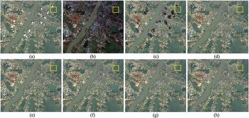
Figure 18. The zoomed details of Figure 17. (a)–(h) are the details of the red rectangle area in Figure 17(a–h). (i)–(p) are the details of the yellow rectangle area in Figure 17(a–h).

Figure 18(a–h) show the zoomed results of the red rectangle area in Figure 17(a–h), respectively, and Figure 18(i–p) show the zoomed results of the yellow rectangle area in Figure 17(a–h), respectively. The result of simply replacement shown in Figure 18(c) denotes the significant radiometric differences between original image and reference image. Figure 18(d) looks much better than Figure 18(c), but there is a color anomaly in the yellow rectangle area, which may be caused by the large difference between images at that location. In the result after boundary optimization, as shown in Figure 18(e), this problem has been relieved. However, in the yellow rectangle area in Figure 18(e), the color is still inconsistent with the color of other area. In Figure 18(f), the differences between various ground features are reduced, resulting in obvious blurring. The color in Figure 18(g) is more harmonious, but some details in the yellow rectangle area are unclear. The result in Figure 18(h), which is reconstructed by the proposed method, shows better radiometric consistency and clearer details. The color of the building in the yellow rectangle area in Figure 18(l) is a little abnormal, because the boundary of cloud coverage area passes through the building, and this problem is alleviated after boundary optimization, as shown in Figure 18(m). However, in the yellow rectangle area in Figure 18(m), the replacement area looks darker than the others, which also occurs in Figure 18(l). The color consistencies of Figure 18(n–o) are better, but the details are slightly blurred, as shown in the yellow rectangle areas. Figure 18(p) shows a more satisfactory result with high color consistency and clear details.

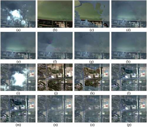
L2A level Sentinel-2A images with 20 m spatial resolution were used as experimental data to test the applicability of the proposed method to multispectral images. The images are composed of 10 bands (band 1: coastal aerosol, band 2: blue, band 3: green, band 4: red, band 5: Vegetation Red Edge (VRE), band 6: VRE, band 7: VRE, band 8: NIR, band 9: Short-wave Infrared (SWIR), band 10: SWIR). Figure 19 shows the experimental data of false color composition using blue, green and NIR bands. Figure 19(a,b) are the cloud-contaminated image and reference image, respectively. Figure 19(c) shows the cloud removal result of the proposed method. Though obvious color differences can be observed between Figure 19(a,b), the cloud removal result in Figure 19(c) still shows a satisfactory color consistency. According to the zoomed results of the yellow rectangle areas in Figure 19, Figure 19(c) well retains the details of the reference image, and transitions naturally at the cloud boundary with a high spatial continuity. More information of each band is further shown in Figure 20. Figure 20(a–j), respectively, shows the experimental data of band 1-band 10. Taking Figure 20(a) as an example, the three images from top to bottom are the cloud-contaminated image, the reference image, and the cloud removal result of the proposed method, respectively, and the zoomed results of the yellow rectangle areas are also shown below. Obviously, the missing area in each band of cloud-contaminated image is well restored with the auxiliary information from the same band of reference image, which also demonstrates the effectiveness of the proposed method for multispectral images.

Figure 19. Sentinel-2A images for real data experiment. (a) Cloud-contaminated image. (b) Reference image. (c) Result of the proposed method.

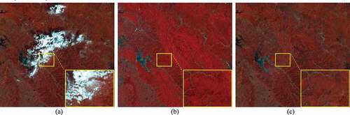
Figure 20. The experimental data of each band. (a) Band 1: Coastal aerosol. (b) Band 2: blue. (c) Band 3: green. (d) Band 4: red. (e) Band 5: VRE. (f) Band 6: VRE. (g) Band 7: VRE. (h) Band 8: NIR. (i) Band 9: SWIR. (j) Band 10: SWIR.

As shown in these experimental results above, the proposed curvature-driven cloud removal method can generate a satisfactory result for images with different resolutions and different scenes. It is known that the simplest way for cloud removal is to directly replace the cloud coverage area in cloud-contaminated image with the corresponding area in reference image. However, there may be obvious color inconsistency in the result of direct replacement method because of the radiometric differences between images caused by various atmospheric situations, such as the results shown in Figure 18(c,k). So it is necessary to make some transformations or reduce the radiometric differences before replacement. The strategy of the proposed method is to perform cloud coverage area replacement in curvature domain rather than nature domain. For most replacement methods, when the cloud boundary passes through the ground features with great radiometric differences between cloud-contaminated image and reference image, the reconstructed result is likely to appear discontinuity at the boundary of replacement area, such as the results of Poisson blending method shown in Figure 8(d). Therefore, after mean curvature transformation, the next step of the proposed method is to optimize the boundary for cloud coverage area replacement. Since the proposed method performs replacement in curvature domain, the boundary consisting of pixels with minimum curvature difference between cloud-contaminated image and reference image is determined as the optimal boundary. As shown in Figure 18(p), the transition at the boundary of replacement area is more natural. When there are significant radiometric differences between cloud-contaminated image and reference image and the radiometric differences are affected by various ground feature classes, it is difficult to guarantee the overall radiometric consistency of the reconstructed image only using the information of cloud covered area. As shown in Figures 8(e) and 16(m), the colors of the reconstructed area and other areas in the image are not harmonious, because the same ground features in the whole image are not uniform in color. Hence, the proposed method utilizes the specific checkpoints, which are pixels that have both the true value from cloud-contaminated image and the reconstructed value from reference image, to further refine the initial cloud-free result. As shown in Figures 8(h) and 16(p), these reconstructed images of the proposed method are more continuous and uniform in color, so the reconstructed area and other areas in the result are naturally integrated into a whole. The quantitative analyses in the simulated experiments also demonstrate that the proposed method can generate satisfactory results with high reconstruction accuracy under different cloud coverage conditions, even if the percentage of cloud coverage in the image reaches 90%, as shown in Figures 13 and 14.

4. Conclusions

The existence of clouds in satellite images is always unavoidable, and the missing area obscured by clouds is a major obstacle to information extraction, which significantly reduces the availability of remote-sensing data. Therefore, in order to make full use of the information from the cloud-free area in the image to be reconstructed, this paper presents a novel curvature-driven cloud removal method for missing area reconstruction of cloud-contaminated images. In the proposed method, images are transformed from natural domain to curvature domain for information reconstruction, and then transformed back to natural domain. The proposed method mainly includes four steps. First, the images are transformed from natural domain to curvature domain by mean curvature transformation. Second, the optimal boundary for cloud coverage area replacement is determined based on the curvature differences between images to make the result transition naturally at the boundary of replacement area. Third, the curvature of missing area in cloud-contaminated image is reconstructed with curvature of corresponding area in reference image, and the reconstructed curvature map is transformed back to natural domain based on curvature equations to generate initial cloud-free result. Considering the possible significant radiometric differences between different images, there may still be slight color inconsistency in the initial cloud-free result. Therefore, the last step is to further refine the initial cloud-free result based on the deviation between the true value and the reconstructed value of specific checkpoints. In addition, both simulated experiments and real data experiments are conducted to demonstrate the strength of the proposed method. Qualitative and quantitative analyses of experimental results have verified that the proposed method can generate high reconstruction accuracy results with good spectral consistency and spatial continuity.

However, there are still a few deficiencies that need to be improved. First, the cloud mask is required to determine the area to be restored, so the proposed method is dependent on the cloud detection result. If the cloud mask is accurate and the cloud coverage area is completely contained, the proposed method can obtain satisfactory cloud removal results for both thick and thin clouds. Otherwise, if the cloud coverage area is not fully detected, the performance of the proposed method will be affected. Second, when a relatively smooth feature is in the cloud-contaminated image, such as the river, and the color difference between the feature and its surrounding feature in the cloud-contaminated image is inconsistent with that in the reference image, the color gradient will occur inside the smooth feature to achieve a global optimization, as shown in Figure 16(g). This is inevitable when the curvature convolution operation is used to approximate the curvature of discrete image, and this problem also exists in Poisson blending method, which uses the divergence operator to calculate the gradient field of images. These problems will be studied in the future.

Disclosure statement

No potential conflict of interest was reported by the author(s).

Data availability statement

The experimental data used in this study can be accessed here: http://36.112.130.153:7777/#/home; https://scihub.copernicus.eu/dhus/#/home.

Additional information

Funding

This work was supported by the National Natural Science Foundation of China [grant number 41971422 and 42090011], Key Research and Development Plan Project of Hubei Province [grant number 2020BIB006], Hubei Provincial Natural Science Foundation [grant number 2020CFA001], and LIESMARS Special Research Funding.

Notes on contributors

Xiaoyu Yu

XiaoyuYu received her B.S. degree at the School of Geosciences and Info-physics, Central South University. She is currently a Ph.D. student at the State Key Laboratory of Information Engineering in Surveying, Mapping and Remote-Sensing, Wuhan University. Her research interests include remote-sensing image reconstruction and image fusion.

Jun Pan

Jun Pan is a professor at the State Key Laboratory of Information Engineering in Surveying, Mapping, and Remote Sensing, Wuhan University. He received the PhD degree from Wuhan University in 2008. His research interests include remote-sensing data intelligent processing and image quality improvement.

Mi Wang

Mi Wang is a professor at the State Key Laboratory of Information Engineering in Surveying, Mapping, and Remote Sensing, Wuhan University. He received the PhD degree from Wuhan University in 2001. His research interests include high-resolution remote-sensing satellite ground processing and the integration and rapid update of photogrammetry and GIS.

Jiangong Xu

XiaoyuYu received her B.S. degree at the School of Geosciences and Info-physics, Central South University. She is currently a Ph.D. student at the State Key Laboratory of Information Engineering in Surveying, Mapping and Remote-Sensing, Wuhan University. Her research interests include remote-sensing image reconstruction and image fusion.

Jiangong Xu received his M.S. degree in ecology from Anhui University in 2022. He is now pursuing his PhD degree in resources and environment at Wuhan University. His research interests include multi-source remote-sensing data fusion based on deep learning.

References

- Atkinson, P. M., P. J. Curran, and R. Webster. 1990. “Sampling Remotely Sensed Imagery for Storage, Retrieval, and Reconstruction.” The Professional Geographer 42 (3): 345–353. doi:10.1111/j.0033-0124.1990.00345.x.
- Cheng, Q., H. Shen, L. Zhang, Q. Yuan, and Z. Chao. 2014. “Cloud Removal for Remotely Sensed Images by Similar Pixel Replacement Guided with a Spatio-Temporal MRF Model.” Isprs Journal of Photogrammetry & Remote Sensing 92 (jun.): 54–68. doi:10.1016/j.isprsjprs.2014.02.015.
- Criminisi, A., P. Perez, and K. Toyama. 2004. “Region Filling and Object Removal by Exemplar-Based Image Inpainting.” IEEE Transactions on Image Processing 13 (9): 1200–1212. doi:10.1109/TIP.2004.833105.
- Dong, Z., M. Wang, D. Li, Y. Wang, and Z. Zhang. 2019. “Cloud Detection Method for High Resolution Remote Sensing Imagery Based on the Spectrum and Texture of Superpixels.” Photogrammetric Engineering & Remote Sensing 85 (4): 257–268. doi:10.14358/PERS.85.4.257.
- Ebel, P., Y. Xu, M. Schmitt, and X. X. Zhu. 2022. “Sen12MS-CR-TS: A Remote-Sensing Data Set for Multimodal Multitemporal Cloud Removal.” IEEE Transactions on Geoscience and Remote Sensing 60: 1–14. doi:10.1109/TGRS.2022.3146246.
- Fang, Z., X. Yu, J. Pan, N. Fan, H. Wang, and J. Qi. 2021. “A Fast Image Mosaicking Method Based on Iteratively Minimizing Cloud Coverage Areas.” IEEE Geoscience and Remote Sensing Letters 18 (8): 1371–1375. doi:10.1109/LGRS.2020.2998920.
- Feng, C., J. W. Ma, Q. Dai, and X. Chen. 2004. ”An Improved Method for Cloud Removal in ASTER Data Change Detection.” IGARSS 2004. 2004 IEEE International Geoscience and Remote Sensing Symposium, Anchorage, AK, USA, pp. 3387–3389 vol.5. doi: 10.1109/IGARSS.2004.1370431.
- Gladkova, I., M. D. Grossberg, F. Shahriar, G. Bonev, and P. Romanov. 2012. “Quantitative Restoration for MODIS Band 6 on Aqua.” IEEE Transactions on Geoscience and Remote Sensing 50 (6): 2409–2416. doi:10.1109/TGRS.2011.2173499.
- Gong, Y. H., and O. Goksel. 2019. “Weighted Mean Curvature.” Signal Processing 164: 329–339. doi:10.1016/j.sigpro.2019.06.020.
- Gong, Y. H., and I. F. Sbalzarini. 2017. “Curvature Filters Efficiently Reduce Certain Variational Energies.” IEEE Transactions on Image Processing 26 (4): 1786–1798. doi:10.1109/tip.2017.2658954.
- Guillemot, C., and O. Le Meur. 2014. “Image Inpainting: Overview and Recent Advances.” Signal Processing Magazine 31 (1): 127–144. doi:10.1109/MSP.2013.2273004.
- Helmer, E. H., and B. Ruefenacht. 2005. “Cloud-Free Satellite Image Mosaics with Regression Trees and Histogram Matching.” Photogrammetric Engineering & Remote Sensing 71 (9): 1079–1089. doi:10.14358/PERS.71.9.1079.
- Hu, C., L. Huo, Z. Zhang, and P. Tang. 2019. ”Automatic Cloud Removal from Multi-Temporal Landsat Collection 1 Data Using Poisson Blending.” IGARSS 2019 - 2019 IEEE International Geoscience and Remote Sensing Symposium, Yokohama, Japan, pp. 1661–1664. doi: 10.1109/IGARSS.2019.8899849.
- Jia, J. Y., J. Sun, C. K. Tang, and H. Y. Shum. 2006. “Drag-And-Drop Pasting.” ACM Transactions on Graphics 25 (3): 631–636. doi:10.1145/1141911.1141934.
- Ju, J., and D. P. Roy. 2008. “The Availability of Cloud-Free Landsat ETM+ Data Over the Conterminous United States and Globally.” Remote Sensing of Environment 112 (3): 1196–1211.
- Kang, Y., L. Pan, Q. Chen, T. Zhang, S. Zhang, and Z. Liu. 2016. “Automatic Mosaicking of Satellite Imagery Considering the Clouds.” ISPRS Annals of the Photogrammetry, Remote Sensing and Spatial Information Sciences III-3: 415–421. doi:10.5194/isprs-annals-III-3-415-2016.
- King, M. D., S. Platnick, W. P. Menzel, S. A. Ackerman, and P. A. Hubanks. 2013. “Spatial and Temporal Distribution of Clouds Observed by MODIS Onboard the Terra and Aqua Satellites.” IEEE Transactions on Geoscience & Remote Sensing 51 (7): 3826–3852. doi:10.1109/TGRS.2012.2227333.
- Kulkarni, S. C., and P. P. Rege. 2020. “Pixel Level Fusion Techniques for SAR and Optical Images: A Review - ScienceDirect.” Information Fusion 59: 13–29. doi:10.1016/j.inffus.2020.01.003.
- Lai, K. -H., and C. -H. Lin. 2012. ”An Optimal Boundary Determination Approach for Cloud Removal in Satellite Image.” 2012 IEEE International Geoscience and Remote Sensing Symposium, Munich, Germany, pp. 2241–2244. doi: 10.1109/IGARSS.2012.6351053.
- Li, M., S. C. Liew, and L. K. Kwoh. 2003. ”Producing Cloud Free and Cloud-Shadow Free Mosaic from Cloudy IKONOS Images.” IGARSS 2003. 2003 IEEE International Geoscience and Remote Sensing Symposium. Proceedings (IEEE Cat. No.03CH37477), Toulouse, France, pp. 3946–3948 vol. 6. doi: 10.1109/IGARSS.2003.1295323.
- Lin, C. H., P. H. Tsai, K. H. Lai, and J. Y. Chen. 2013. “Cloud Removal from Multitemporal Satellite Images Using Information Cloning.” IEEE Transactions on Geoscience & Remote Sensing 51 (1): 232–241. doi:10.1109/TGRS.2012.2197682.
- Li, D., J. Shan, Z. Shao, X. Zhou, and Y. Yao. 2013. “Geomatics for Smart Cities - Concept, Key Techniques, and Applications.” Geo-Spatial Information Science 16 (1): 13–24. doi:10.1080/10095020.2013.772803.
- Li, X., H. Shen, L. Zhang, H. Zhang, and Q. Yuan. 2014. “Dead Pixel Completion of Aqua MODIS Band 6 Using a Robust M-Estimator Multiregression.” IEEE Geoscience and Remote Sensing Letters 11 (4): 768–772. doi:10.1109/LGRS.2013.2278626.
- Liu, X. G., H. J. Bao, and Q. S. Peng. 2006. “Digital Differential Geometry Processing.” Journal of Computer Science and Technology 21 (5): 847–860. doi:10.1007/s11390-006-0847-5.
- Li, D., M. Wang, and J. Jiang. 2021. “China’s High-Resolution Optical Remote Sensing Satellites and Their Mapping Applications.” Geo-Spatial Information Science 24 (1): 85–94. doi:10.1080/10095020.2020.1838957.
- Li, J., Z. Wu, Z. Hu, J. Zhang, M. Molinier, L. Mo, and M. Molinier. 2020. “Thin Cloud Removal in Optical Remote Sensing Images Based on Generative Adversarial Networks and Physical Model of Cloud Distortion.” Isprs Journal of Photogrammetry and Remote Sensing 166: 373–389. doi:10.1016/j.isprsjprs.2020.06.021.
- Li, J., Z. Wu, Q. Sheng, B. Wang, Z. Hu, S. Zheng, G. Camps-Valls, and M. Molinier. 2022. “A Hybrid Generative Adversarial Network for Weakly-Supervised Cloud Detection in Multispectral Images.” Remote Sensing of Environment 280: 113197. doi:10.1016/j.rse.2022.113197.
- Maalouf, A., P. Carre, B. Augereau, and C. Fernandez-Maloigne. 2009. “A Bandelet-Based Inpainting Technique for Clouds Removal from Remotely Sensed Images.” IEEE Transactions on Geoscience & Remote Sensing 47 (7): 2363–2371. doi:10.1109/TGRS.2008.2010454.
- Meng, Q., B. E. Borders, C. J. Cieszewski, and M. Madden. 2009. “Closest Spectral Fit for Removing Clouds and Cloud Shadows.” Photogrammetric Engineering & Remote Sensing 75 (5): 569–576. doi:10.14358/PERS.75.5.569.
- Meng, X., H. Shen, Q. Yuan, H. Li, L. Zhang, and W. Sun. 2019. “Pansharpening for Cloud-Contaminated Very High-Resolution Remote Sensing Images.” IEEE Transactions on Geoscience and Remote Sensing 57 (5): 2840–2854. doi:10.1109/TGRS.2018.2878007.
- Meraner, A., P. Ebel, X. Zhu, and M. Schmitt. 2020. “Cloud Removal in Sentinel-2 Imagery Using a Deep Residual Neural Network and SAR-Optical Data Fusion.” Isprs Journal of Photogrammetry and Remote Sensing 166: 333–346. doi:10.1016/j.isprsjprs.2020.05.013.
- Mitchell, O. R., E. J. Delp, and P. L. Chen. 1977. “Filtering to Remove Cloud Cover in Satellite Imagery.” IEEE Transactions on Geoscience Electronics 15 (3): 137–141. doi:10.1109/TGE.1977.6498971.
- Park, S., X. Guo, H. Shin, and Q. Hong. 2005. ”Shape and Appearance Repair for Incomplete Point Surfaces.” Tenth IEEE International Conference on Computer Vision (ICCV'05) Volume 1, Beijing, China, pp. 1260–1267 Vol. 2. doi: 10.1109/ICCV.2005.218.
- Perez, P., M. Gangnet, and A. Blake. 2003. “Poisson Image Editing.” ACM Transactions on Graphics 22 (3): 313–318. doi:10.1145/882262.882269.
- Rossi, R. E., J. L. Dungan, and L. R. Beck. 1994. “Kriging in the Shadows: Geostatistical Interpolation for Remote Sensing.” Remote Sensing of Environment 49 (1): 32–40. doi:10.1016/0034-4257(94)90057-4.
- Sarukkai, V., A. Jain, B. Uzkent, and S. Ermon. 2020. ”Cloud Removal in Satellite Images Using Spatiotemporal Generative Networks.” 2020 IEEE Winter Conference on Applications of Computer Vision (WACV), Snowmass, CO, USA. pp. 1785–1794. doi: 10.1109/WACV45572.2020.9093564.
- Sebastianelli, A., A. Nowakowski, E. Puglisi, M. Rosso, J. Mifdal, F. Pirri, P. P. Mathieu, and S. L. Ullo. 2021. “Spatio-Temporal SAR-Optical Data Fusion for Cloud Removal via a Deep Hierarchical Model.” arXiv preprint arXiv:2106.12226.
- Shen, H., X. Li, Q. Cheng, C. Zeng, G. Yang, H. Li, and L. Zhang. 2015. “Missing Information Reconstruction of Remote Sensing Data: A Technical Review.” IEEE Geoscience & Remote Sensing Magazine 3 (3): 61–85. doi:10.1109/MGRS.2015.2441912.
- Shen, H., C. Zeng, and L. Zhang. 2011. “Recovering Reflectance of AQUA MODIS Band 6 Based on Within-Class Local Fitting.” IEEE Journal of Selected Topics in Applied Earth Observations & Remote Sensing 4 (1): 185–192. doi:10.1109/JSTARS.2010.2077620.
- Shen, H., and L. Zhang. 2009. “A MAP-Based Algorithm for Destriping and Inpainting of Remotely Sensed Images.” IEEE Transactions on Geoscience and Remote Sensing 47 (5): 1492–1502. doi:10.1109/TGRS.2008.2005780.
- Tao, C., S. Fu, J. Qi, and H. Li. 2022. “Thick Cloud Removal in Optical Remote Sensing Images Using a Texture Complexity Guided Self-Paced Learning Method.” IEEE Transactions on Geoscience and Remote Sensing 60: 1–12. doi:10.1109/TGRS.2022.3157917.
- Wang, Z., J. Jin, J. Liang, K. Yan, and Q. Peng. 2005. “A New Cloud Removal Algorithm for Multi-Spectral Images.“ In L. Zhang, J. Zhang, and M. Liao (Eds.), Proceedings of the MIPPR 2005: SAR Multispectral Image Process, Wuhan, China, p. 60430. doi:10.1117/12.654869.
- Wang, Z., E. P. Simoncelli, and A. C. Bovik. 2003. ”Multiscale Structural Similarity for Image Quality Assessment.” The Thrity-Seventh Asilomar Conference on Signals, Systems & Computers, 2003, Pacific Grove, CA, USA, pp. 1398–1402 Vol. 2. doi: 10.1109/ACSSC.2003.1292216.
- Zeng, C., H. Shen, and L. Zhang. 2013. “Recovering Missing Pixels for Landsat ETM + SLC-Off Imagery Using Multi-Temporal Regression Analysis and a Regularization Method.” Remote Sensing of Environment 131: 182–194.
- Zhang, Y., B. Guindon, and J. Cihlar. 2002. “An Image Transform to Characterize and Compensate for Spatial Variations in Thin Cloud Contamination of Landsat Images.” Remote Sensing of Environment 82 (2): 173–187. doi:10.1016/S0034-4257(02)00034-2.
- Zhang, Q., Q. Yuan, J. Li, Z. Li, H. Shen, and L. Zhang. 2020. “Thick Cloud and Cloud Shadow Removal in Multitemporal Imagery Using Progressively Spatio-Temporal Patch Group Deep Learning.” Isprs Journal of Photogrammetry and Remote Sensing 162: 148–160. doi:10.1016/j.isprsjprs.2020.02.008.
- Zhang, Q., Q. Yuan, Z. Li, F. Sun, and L. Zhang. 2021. “Combined Deep Prior with Low-Rank Tensor SVD for Thick Cloud Removal in Multitemporal Images.” Isprs Journal of Photogrammetry and Remote Sensing 177: 161–173. doi:10.1016/j.isprsjprs.2021.04.021.
- Zhang, Q., Q. Yuan, C. Zeng, X. Li, and Y. Wei. 2018. “Missing Data Reconstruction in Remote Sensing Image with a Unified Spatial–Temporal–Spectral Deep Convolutional Neural Network.” IEEE Transactions on Geoscience and Remote Sensing 56 (8): 4274–4288. doi:10.1109/TGRS.2018.2810208.
- Zhou, W., and A. C. Bovik. 2002. “A Universal Image Quality Index.” IEEE Signal Processing Letters 9 (3): 81–84. doi:10.1109/97.995823.
- Zhu, W., and T. Chan. 2012. “Image Denoising Using Mean Curvature of Image Surface.” SIAM Journal on Imaging Sciences 5 (1): 1–32. doi:10.1137/110822268.