Perimeter-Area Soil Carbon Index (PASCI): modeling and estimating soil organic carbon using relevant explicatory waveband variables in machine learning environment

ABSTRACT

Soil Organic Carbon (SOC) is the most important indicator of soil health and determines long-term crop productivity. Here, we applied the Random Forest regression model to soil hyperspectral data to determine the important spectral bands and regions for SOC retrieval. Multiple existing studies already identified specific wavelength bands that could be good indicators of SOC. However, there is no hyperspectral-based method that is currently available to simultaneously investigate these identified specific wavelength regions for SOC. To help fill this gap, we developed the Perimeter-Area Soil Carbon Index (PASCI) that utilized optimal SOC spectral bands and then evaluated its robustness for SOC prediction and retrieval against other existing indices. The results of regression analysis between SOC and PASCI values showed a significant relationship (r² = 0.76; p < 0.05). A significant statistical relationship (r² = 0.73) was also observed between SOC and the sum indices. The results from this study have advanced our understanding of the optimal spectral bands for SOC. Finally, the PASCI could be applied to hyperspectral and multispectral images to remotely quantify, predict, and map SOC.

KEYWORDS:

• Soil carbon index
• hyperspectral index
• random forest
• soil carbon prediction

1. Introduction

Soil carbon is regarded as a critical soil quality characteristic that determines soil health for long-term crop productivity (Oldfield, Bradford, and Wood 2019). The quantity of Soil Organic Carbon (SOC) impacts various soil qualities and activities, including aggregate stability, water-holding capacity, microbial activity, and soil nutrient fertility, all of which are important for long-term crop development. SOC estimation, assessment, and monitoring allow for the creation of effective site-specific crop management methods that will sustain crop output and assure global food security (Brown and Funk 2008; Kaya et al. 2022).

To estimate SOC, the use of Hyperspectral Sensors (HS) is the more contemporary approach. Compared to the traditional approach, the HS approach uses empirical calibration equations that relate the findings of traditional analysis to soil spectrum chromophores displaying the soil attribute of interest. One of the characteristics of HS is its capability to characterize a physical soil property, such as SOC, in a high spectral resolution. The contiguous spectral bands of HS could provide a vast amount of information that are useful for precision agriculture (Khanal, Fulton, and Shearer 2017), estimation of net primary productivity (Ruimy, Dedieu, and Saugier 1996) and monitoring the effects of management and land use practices on soil organic matter content (Selige, Böhner, and Schmidhalter 2006). In carbon cycle assessment, hyperspectral reflectance signatures from soil have been shown to contain a wide range of physical and chemical information (Cozzolino and Moron 2003).

Reflectance spectra from the remote sensing dataset could provide possible Soil Carbon Indices (SCI) because of the presence of absorption characteristics in the visible, near-infrared (NIR) and mid-infrared (MIR) portions of the electromagnetic spectrum. These SCIs typically are derived using the ratio and difference of wavelength bands that are inherent in the remote sensing data. The optimal wavebands that could offer a good measure of the SOC are roughly approximated to be 700 nm to 950 nm and 1097 nm to 2183 nm (Sorenson, Quideau, and Rivard 2017). Other specific spectral positions for soil carbon have also been identified occurring in the visible region: 587 nm and 585.9 nm (Islam, Singh, and McBratney 2003), 540 nm and 550 nm (Brown et al. 2006); and the SWIR region: 1940 nm and 2180 nm (Vågen, Shepherd, and Walsh 2006).

Most studies have investigated the visible to mid-infrared reflectance to correctly determine SOC. Murray and Williams (1987) found a broad region from 400 to 2498 nm, Reeves (1996) found the range 4000 – 400 cm⁻¹, and Kooistra et al. (2003) indicated important wavelength on 530 nm, 1970 nm, 2180 nm, 2280 nm, and 2360 nm. More recent studies found significant wavelength regions associated with SOC: Qiao et al. (2017) (417 nm, 1853 nm, 1000 nm, and 2412 nm); Sorenson, Quideau, and Rivard (2017) (700 nm–950 nm and 1097 nm–2183 nm); Sun, Li, and Niu (2018) (750 nm–2450 nm); Šestak et al. (2018) (670 nm–710 nm and 730 nm–770 nm). However, there is no hyperspectral-based index that is currently available to simultaneously investigate these identified wavelength regions for SOC. Therefore, we propose to develop a novel approach that would simultaneously use various important spectral regions to characterize SOC effectively. In this work, we sought to establish a novel spectral index by using hyperspectral data that could guide SOC predictions. The aims of this study were (1) to determine the important spectral bands and regions for SOC retrieval, (2) to develop a hyperspectral soil carbon index using important spectral bands, and (3) to evaluate the robustness of the new index for SOC prediction and retrieval against other existing SOC indices. We expect that the new index would be useful in generating a map of SOC using open-access airborne and satellite images. While the new index would be useful for hyperspectral images, we also see its application for multispectral sensors such as Sentinel imagery from the European Space Agency (ESA) and Landsat series from the National Aeronautics and Space Administration (NASA).

2. Methods

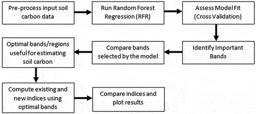
Figure 1 provides the overall flow of the adopted methodology, which is divided into eight important steps.

Figure 1. A general flowchart of the methodology, starting from preprocessing the dataset to analysis, and finally plotting the results.

2.1. Soil carbon and spectral dataset

We utilized the soil carbon and spectral datasets that are publicly available for download from the Natural Resources Conservation Service’s (NRCS) Soil Science Division, Rapid Carbon Assessment (RaCA) project website (Soil Survey Staff 2013). The RaCA was initiated to provide a scientifically and statistically defensible inventory of soil carbon stocks across different U.S. regions and further stratified by a combination of soil groups and land use/land cover classes (Wills et al. 2014). More than 300 soil scientists participated in sample collection and analysis, with assistance from 24 universities. We used a total of 672 SOC samples from the upper 1 m soil profiles that also have available pairs of laboratory Visible-Near Infrared (VNIR) spectra. The VNIR spectra have a range of 350 nm to 2500 nm, acquired at 1 nm increments. We used these SOC and VNIR spectra data pairs to build a SOC predictive model. Specific details of the methods and sampling used in the collection of the RaCA dataset could be found in Wills et al. (2014). As part of the pre-processing, we formatted the dataset for use as input to our modeling algorithm by deleting data columns that we did not need and kept only the spectral bands and the SOC records.

2.2. Random forest regression model and assessment

We used the Random Forest (RF) regression model to quantify the relationship between SOC samples and their corresponding spectral reflectance (Biau and Scornet 2016). RF is a non-parametric machine learning approach that combines a large number of decision trees, resulting in a smaller variance (Breiman 2001; Keshavarzi et al. 2022). Each RF tree is constructed using the Classification and Regression Tree (CART) technique and the Decrease Gini Impurity (DGI) as the splitting criterion, using a bootstrap sample taken at random from the original dataset. The RF model works by partitioning the space of the input VNIR spectral variables into regions such that the variation in SOC within the same region is relatively small. The analysis produces two independent partitions of the space of variables. CART works by allowing for all possible splits on all potential explanatory spectral variables. One of the outputs of the regression model is a ranking of spectral variable importance (Van der Laan 2006).

We chose RF among other models for several advantages: (1) simplicity in model parameterization (Pal 2005), (2) control of predictor variables (Evans et al. 2011), (3) a robust method for the selection of hyperspectral bands (Genuer, Poggi, and Tuleau-Malot 2010), and (4) low correlation among trees and avoids over-fitting (Salas and Subburayalu 2019). Also, RF regression performed best when compared to other regression approaches (Couronné, Probst, and Boulesteix 2018). RF has also been shown to be effective for mapping SOC using Sentinel 2 images (Albert and Ammar 2021; Urbina-Salazar et al. 2021). The model was implemented in the R statistical environment using the packages randomForest, caret, plyr, and e1071 (Liaw and Wiener 2002).

We assessed the performance of the model by using leave-one-out cross-validation instead of the train/test split validation method since the former is more robust to confounding model effects (Saeb et al. 2017). We trained the model n times, where n is the number of samples, with one sample discarded for testing each time. This method produced model performance estimates that are similar to out-of-bag error and mean of squared residuals (Liaw and Wiener 2002). Model performance metrics include r², Root Mean Squared Error (RMSE), and m, Mean Absolute Error (MAE) (Salas et al. 2022).

2.3. Perimeter-Area Soil Carbon Index (PASCI)

From the ranking of spectral variable importance, we used the optimal spectral bands previously identified for SOC to develop a new index. The unitless Perimeter-Area Soil Carbon Index (PASCI) (Equation (1)(1) $PASCI=\frac{\frac{P}{A}-min\frac{P}{A}}{max\frac{P}{A}-min\frac{P}{A}}$(1) ) takes advantage of the multiple optimal spectral bands by calculating perimeters and areas based on the gradient principle. PASCI is the normalized ratio of the perimeter and area circumscribed by it that is under the straight line connecting the spectral maxima of each optimum band (see hypothetical Figure 2).

Figure 2. A sample diagram to visualize the components of the Perimeter-Area Soil Carbon Index (PASCI). b1 is the average of all reflectance values from 370 to 390 nm; b2 is the average of all reflectance values from 400 to 410 nm; b3 is the average of all reflectance values from 1120 to 1125 nm; b4 is the average of all reflectance values from 1400 to 1410; b5 is the average of all reflectance values from 1540 to 1545 nm; and b6 is the reflectance value of band 2315 nm.

(1) $PASCI=\frac{\frac{P}{A}-min\frac{P}{A}}{max\frac{P}{A}-min\frac{P}{A}}$(1)

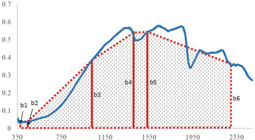
where P represents the total outer perimeter of the shaded polygon, represented by a dashed line. A represents the total area of the shaded polygon. Variables b1 to b6 represent reflectance values. b1 is the average of all reflectance values from 370 to 390 nm; b2 is the average of all reflectance values from 400 to 410 nm; b3 is the average of all reflectance values from 1120 to 1125 nm; b4 is the average of all reflectance values from 1400 to 1410; b5 is the average of all reflectance values from 1540 to 1545 nm; and b6 is the reflectance value of band 2315 nm.

The total area, A, is computed by summing up the areas of small trapezoids (Figure 3). To compute the area of one trapezoid (Equation (2)(2) $A_i=\left\{0.5\left(\mathrm{\Delta }x1\right)\left(\mathrm{\Delta }y3\right)\right\}+\left\{\left(\mathrm{\Delta }y1\right)\left(\mathrm{\Delta }y2\right)\right\}$(2) ) and the total area (Equation (3)(3) $A={\sum }_{i=1}^n{A}_i$(3) ):

Figure 3. A sample magnified trapezoid from Figure 2, shows the dimensions and the peripheral area. There are five (5) small trapezoids like this that compose the total area in Figure 2.

(2) $A_i=\left\{0.5\left(\mathrm{\Delta }x1\right)\left(\mathrm{\Delta }y3\right)\right\}+\left\{\left(\mathrm{\Delta }y1\right)\left(\mathrm{\Delta }y2\right)\right\}$(2)

(3) $A={\sum }_{i=1}^n{A}_i$(3)

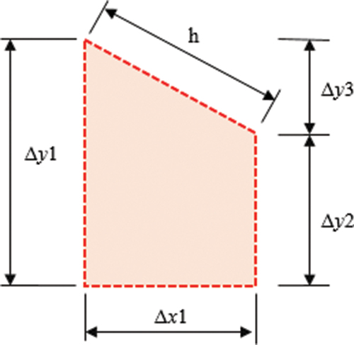
where Δx and Δy are the dimensions of the trapezoid, A_i is the area of each trapezoid, A is the total area of the polygon.

The total outer perimeter, P, is computed by summing up the lengths of all dashed lines or boundaries (Figure 2). For inclined lines, the Pythagorean theorem is applied (Equation (4)(4) $h=\sqrt{{\left(\mathrm{\Delta }y3\right)}^2+{\left(\mathrm{\Delta }y1-\mathrm{\Delta }y2\right)}^2}$(4) ).

(4) $h=\sqrt{{\left(\mathrm{\Delta }y3\right)}^2+{\left(\mathrm{\Delta }y1-\mathrm{\Delta }y2\right)}^2}$(4)

where h is the length of the inclined line, $\mathrm{\Delta }y$ represents the dimension of the trapezoid (could also mean the reflectance values or difference of reflectance values) (Figure 3).

The PASCI algorithm includes all optimal spectral bands for SOC to address the limitations of other current SOC indices, which only use two or three ideal bands. PASCI is designed to identify the small variations of the area that are caused by absorption features within the periphery bounded by all bands. The PASCI differentiates itself from the continuum removed function (Grove, Hook, and Paylor 1992) in that the former includes the P component, which is influenced by the shape and size of A (shaded polygon). While the inclusion of multiple bands could increase model calculation times, the PASCI is constructed to ensure that the A and P could detect as much as relevant spectral variations necessary to predict SOC. Currently, there is no index available to investigate these multiple spectral bands for SOC simultaneously.

2.4. Other existing indices

We compared the performance of PASCI as a SOC predictor against existing SOC hyperspectral indices. The sum indices measure the size of SOC absorption features on specific absorption bands: 1/Sum(top 5 bands) and 1/Sum(top 10 bands) (Grove, Hook, and Paylor 1992). The slope indices measure the change of reflectance between important SOC absorption feature bands: Slope (308 to 405 nm) and Slope (400 to 600 nm) (Bartholomeus et al. 2008). The Moment Distance Index Normalized (MDIN) is a shape index that highlights shape differences in spectral curves (Salas and Subburayalu 2019). Finally, we assessed the quality of the fit for all indices using the r²-value with a confidence level of 0.95.

3. Results

The list of optimal spectral bands in the VIS, NIR, and SWIR electromagnetic (EM) regions for SOC is shown in Table 1. Among the three EM regions, the VIS had the most important predictor bands for SOC, ranging from 370 to 390 nm (>10% increase in Mean Square Error) and 400 to 410 nm (8% to 10% increase in Mean Square Error). Between 370 and 410 nm, bands 380 nm and 390 nm were the most important for SOC. The important bands in the NIR included those in the spectral range 1120 to 1125 nm and 1400 to 1410 nm. The SWIR also registered important SOC predictors, the spectral range 1540 to 1545 nm, and a single band 2315 nm. The RF model obtained an RMSE of 5.16 and MAE of 3.98.

Table 1. A summary of the specific important wavelength regions and optimal spectral bands for prediction and retrieval of SOC.

Optimal Bands in Specific EM Regions
VIS (nm)	NIR (nm)	SWIR (nm)
370–390 400–410	815 995 1120–1125 1400–1410	1540–1545 2315 2485–2500

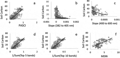
The comparative strengths of the correlations between PASCI and the SOC could provide insights into the effectiveness of the newly developed index. The prediction equations of the models are shown in Table 2. We plotted PASCI as a function of the SOC and found a much higher linear correlation (r² = 0.76) when compared against other indices. In general, PASCI had the best model than 1/Sum (top 5 bands) (r² = 0.73) and 1/Sum (top 10 bands) (r² = 0.73). The MDIN displayed a lower linear correlation than PASCI (r² = 0.36), however, it is comparable to the index Slope (308 to 405 nm).

Table 2. These are the generated regression models and the correlation coefficients between the soil carbon (dependent variable) and the indices (independent variables).

Independent Variables	Model	r^2
PASCI	y = 54.315x − 4.8365	0.76
Slope (308–405 nm)	y = 9.6004e^−2992x	0.36
Slope (400–600 nm)	y = 31.83e^−2239x	0.19
1/Sum(top 5 bands)	y = 63.556x − 11.09	0.73
1/Sum(top 10 bands)	y = 126.62x − 10.98	0.73
MDIN	y = 6.1346x − 6.734	0.36

Figure 4 illustrates the trends of the soil carbon as plotted against the existing indices and PASCI. The slope-based indices are exponentially correlated with SOC, while PASCI, MDIN, and Sums are linearly correlated with SOC.

Figure 4. Scatter plots of the SOC against. (a) PASCI; (b) Slope (308 to 405); (c) Slope (400 to 600); (d) 1/Sum(top 5 bands); (e) 1/Sum(top 10 bands), and (f) MDIN.

4. Discussion

4.1. PASCI vs sum indices

The PASCI is effective at estimating SOC because it captures changes in the reflectance at specific important wavelength regions for SOC. The integration of P and A into PASCI enabled the tracking of the variations of SOC concentrations, such that high values of SOC correlates to high values of PASCI. The equivalent findings of the PASCI and Sum indices demonstrated that using multiple bands in the index could benefit in identifying as many important spectral differences required to predict SOC. However, good correlations found in Sum indices may only be caused by the higher amounts of SOC. In lesser concentrations, the Sum indices may be unable to discern SOC spectral absorption characteristics because absorption from other biological components may predominate (Stoner and Baumgardner 1980). Furthermore, because the PASCI uses P and A, the index removes the limitation of the Sum indices. PASCI measures the object shape, in this case, the size of A (shaded polygon) (Figure 2). By focusing on the shape of A, we eliminated other absorptive features (Oparin et al. 2012), in this case, those features unrelated to SOC. We also reduced the spectral data to the polygon-under-the-curve factor, which is defined only by the optimal bands for SOC. Finally, by concentrating on the shape of A, we captured the subtle variations of spectra so that our model could isolate the local site-specific SOC variations.

4.2. PASCI optimal bands

Our findings on a number of the optimal band locations are consistent with those found by Vohland et al. (2017). The VIS region produced more optimal bands than NIR and SWIR regions. However, the two most important bands for SOC in the visible are 380 nm and 390 nm. These bands have not yet been specifically identified in recent SOC models. Instead, Islam, Singh, and McBratney (2003) and Brown et al. (2006) both acknowledged bands around 500 nm as SOC indicators. Results from Sarkhot et al. (2011) and Qiao et al. (2017) were the closest findings that we could compare our results to, at wavelengths 358 nm and 417 nm, respectively. Similar to Sarkhot et al. (2011), we did not consider a priori the collinearity between bands, because we needed to identify the optimal subset of bands for SOC in the visible, NIR, and SWIR regions. The important NIR band we identified for SOC at 995 nm is consistent with previous studies by Laamrani et al. (2019), located at 998 nm. The bands we identified at 1540 to 1545 nm and 2315 nm that have a large contribution to the SOC prediction model were also within the wavelength ranges presented by Viscarra Rossel and Behrens (2010), Sarkhot et al. (2011), and Laamrani et al. (2019). These parallels in literature findings suggested that the optimal bands identified here could be powerful analytical wavelength bands for determining SOC levels.

4.3. Applicability of PASCI

The PASCI could easily be applied to hyperspectral and multispectral images, where wavelengths in the SWIR region are available, to remotely quantify, predict, and map SOC. When the PASCI equation is used on a multispectral image, the closest waveband that is available should be applied, while missing wavebands could be skipped. The applicability of PASCI on multispectral images is being tested in ongoing research. Creating large-format SOC maps is especially useful for researchers, stakeholders, and policymakers in the agricultural sector. The development of PASCI is timely, with the technological advances in sensors and equipment. PASCI could provide a framework for linking field-based SOC with airborne or satellite remote sensing data. To back up the findings of this study, PASCI should be evaluated utilizing remote sensing data collected from fields with varied management strategies and soil types.

5. Conclusions

In this study, we used 672 samples from the RaCA dataset for the prediction of SOC using the RF regression model. The major conclusions drawn from this study are as follows.

• Non-linear models, such as RF, performed satisfactorily in the SOC band prediction with an RMSE of 5.16 and MAE of 3.98.

• Among all identified optimal spectral bands for SOC, those located in the VIS region have the highest contributions to the SOC model, followed by those in the NIR, and then the SWIR.

• The new PASCI was designed to utilize all the important SOC bands. It showed higher accuracy than other existing SOC indices when we evaluated its robustness for SOC prediction and retrieval.

• The PASCI could be applied to hyperspectral and multispectral images to remotely quantify, predict, and map SOC.

Disclosure statement

No potential conflict of interest was reported by the author(s).

Data availability statement

The soil carbon and spectral datasets used in this study are publicly available for download from the Natural Resources Conservation Service’s (NRCS) Soil Science Division, Rapid Carbon Assessment (RaCA) project website https://www.nrcs.usda.gov/resources/data-and-reports/rapid-carbon-assessment-raca.

Additional information

Funding

This work was supported by the National Aeronautics and Space Administration（Grant number 80NSSC17K0653 P00001） for the joint NASA and Indian Space Research Organization AVIRIS-NG Campaign in India. It was also supported by NIFA/USDA through Central State University Evans-Allen Research Program（Grant Number NI201445×XXXG018-0001）.

Notes on contributors

Eric Ariel L. Salas

Eric Ariel Salas received his BS degree in civil engineering from the University of San Carlos in Cebu, Philippines, and his MSc degree in geo-information from Wageningen University and Research in Wageningen, The Netherlands. He earned his PhD in geospatial science and engineering with a specialization in remote sensing geography from South Dakota State University in Brookings, South Dakota, USA.

Sakthi Subburayalu Kumaran

Sakthi Subburayalu Kumaran has a BS degree in Agriculture and an MSc degree in soil science and agricultural chemistry. He has a PhD in soil science from The Ohio State University in Columbus, Ohio, USA. His research interests include soil and water conservation, data science in digital agriculture, application of machine learning, and remote sensing for precision agricultural management.

References

- Albert, G., and S. Ammar. 2021. “Application of Random Forest Classification and Remotely Sensed Data in Geological Mapping on the Jebel Meloussi Area (Tunisia).” Arabian Journal of Geosciences 14 (21): 2240. doi:10.1007/s12517-021-08509-x.
- Bartholomeus, H. M., M. E. Schaepman, L. Kooistra, A. Stevens, W. B. Hoogmoed, and O. S. P. Spaargaren. 2008. “Spectral Reflectance Based Indices for Soil Organic Carbon Quantification.” Geoderma 145 (1–2): 28–36. doi:10.1016/j.geoderma.2008.01.010.
- Biau, G., and E. Scornet. 2016. “A Random Forest Guided Tour.” TEST 25 (2): 197–227. doi:10.1007/s11749-016-0481-7.
- Breiman, L. 2001. “Random Forests.” Machine Learning 45 (1): 5–32. doi:10.1007/s11749-016-0481-7.
- Brown, D. J., K. D. Shepherd, M. G. Walsh, M. M. Dewayne, and T. G. Reinsch. 2006. “Global Soil Characterization with VNIR Diffuse Reflectance Spectroscopy.” Geoderma, 132: 273–290. doi:10.1016/j.geoderma.2005.04.025.
- Brown, M. E., and C. C. Funk. 2008. “Food Security Under Climate Change.” Science 319 (5863): 580–581. doi:10.1126/science.1154102.
- Couronné, R., P. Probst, and A. L. Boulesteix. 2018. “Random Forest versus Logistic Regression: A Large-Scale Benchmark Experiment.” BMC Bioinformatics 19 (1): 270. doi:10.1186/s12859-018-2264-5.
- Cozzolino, D, and A. Moron. 2003. “The Potential of Near-Infrared Reflectance Spectroscopy to Analyse Soil Chemical and Physical Characteristics.” The Journal of Agricultural Science 140: 65–71. doi:10.1017/S0021859602002836.
- Evans, J., M. Murphy, Z. Holden, and S. Cushman. 2011. “Modeling Species Distribution and Change Using Random Forest.” In Predictive Species and Habitat Modeling in Landscape Ecology, edited by C. A. Drew, Y. F. Wiersma, and F. Huettmann, 139–159. Springer. doi:10.1007/978-1-4419-7390-0_8.
- Genuer, R., J.-M. Poggi, and C. Tuleau-Malot. 2010. “Variable Selection Using Random Forests.” Pattern Recognition Letters 31 (14): 2225–2236. doi:10.1016/j.patrec.2010.03.014.
- Grove, C. I., S. J. Hook, and E. D. Paylor. 1992. “Laboratory Reflectance Spectra of 160 Minerals 0.4 to 2.5 Micrometers.” JPL Publication 92: 406.
- Islam, K., B. Singh, and A. McBratney. 2003. “Simultaneous Estimation of Several Soil Properties by Ultra-Violet, Visible, and Near-Infrared Reflectance Spectroscopy.” Australian Journal of Soil Research 41 (6): 1101–1114. doi:10.1071/SR02137.
- Kaya, F., A. Keshavarzi, R. Francaviglia, G. Kaplan, L. Başayiğit, and M. Dedeoğlu. 2022. “Assessing Machine Learning-Based Prediction Under Different Agricultural Practices for Digital Mapping of Soil Organic Carbon and Available Phosphorus.” Agriculture 12 (7): 1062. doi:10.3390/agriculture12071062.
- Keshavarzi, A., M. Á. S. Del Árbol, F. Kaya, Y. Gyasi-Agyei, and J. Rodrigo-Comino. 2022. “Digital Mapping of Soil Texture Classes for Efficient Land Management in the Piedmont Plain of Iran.” Soil Use and Management 38: 1705–1735. doi:10.1111/sum.12833.
- Khanal, S., J. Fulton, and S. Shearer. 2017. “An Overview of Current and Potential Applications of Thermal Remote Sensing in Precision Agriculture.” Computers and Electronics in Agriculture 139: 22–32. doi:10.1016/j.compag.2017.05.001.
- Kooistra, L., J. Wanders, G. F. Epema, R. S. E. W. Leuven, R. Wehrens, and L. M. C. Buydens. 2003. “The Potential of Field Spectroscopy for the Assessment of Sediment Properties in River Floodplains.” Analytica Chimica Acta 484: 198–200. doi:10.1016/S0003-2670(03)00331-3.
- Laamrani, A., A. A. Berg, P. Voroney, H. Feilhauer, L. Blackburn, M. March, R. C. Martin, Y. He, and R. C. Martin. 2019. “Ensemble Identification of Spectral Bands Related to Soil Organic Carbon Levels Over an Agricultural Field in Southern Ontario, Canada.” Remote Sensing 11 (11): 1298. doi:10.3390/rs11111298.
- Liaw, A., and M. Wiener. 2002. “Classification and Regression by Random Forest.” R News 2: 18–22.
- Murray, I., and P. C. Williams. 1987. “Chemical Principles of Near-Infrared Technology.” In Near Infrared Technology in the Agricultural and Food Industries, American Association of Cereal Chemists, edited by P. C. Williams and K. Norris, 17–34. Minnesota, USA: Inc., St. Paul.
- Oldfield, E., M. A. Bradford, and S. A. Wood. 2019. “Global Meta‐analysis of the Relationship Between Soil Organic Matter and Crop Yields.” Soil 5 (1): 15–32. doi:10.5194/soil-5-15-2019.
- Oparin, V. N., V. P. Potapov, O. L. Giniyatullina, and N. V. Andreeva. 2012. “Water Body Pollution Monitoring in Vigorous Coal Extraction Areas Using Remote Sensing Data.” Journal of Mining Science 48 (5): 934–940. doi:10.1134/S106273914805019X.
- Pal, M. 2005. “Random Forest Classifier for Remote Sensing Classification.” International Journal of Remote Sensing 26 (1): 217–222. doi:10.1080/01431160412331269698.
- Qiao, X. X., C. Wang, M. C. Feng, W. D. Yang, G. W. Ding, H. Sun, Z. Y. Liang, and C. C. Shi. 2017. “Hyperspectral Estimation of Soil Organic Matter Based on Different Spectral Preprocessing Techniques.” Spectroscopy Letters 50 (3): 156–163. doi:10.1080/00387010.2017.1297958.
- Reeves, J. B., III. 1996. “Improvement in Fourier Near-And Mid-Infrared Diffuse Reflectance Spectroscopic Calibration Through the Use of a Sample Transport Device.” Applied Spectroscopy 50 (8): 965–969. doi:10.1366/0003702963905358.
- Ruimy, A., G. Dedieu, and B. Saugier. 1996. “TURC: A Diagnostic Model of Continental Gross Primary Productivity and Net Primary Productivity.” Global Biogeochemical Cycles 10 (2): 269–285. doi:10.1029/96GB00349.
- Saeb, S., L. Lonini, A. Jayaraman, D. C. Mohr, and K. P. Kording. 2017. “The Need to Approximate the Use-Case in Clinical Machine Learning.” GigaScience 6 (5): 1–9. doi:10.1093/gigascience/gix019.
- Salas, E. A. L., S. S. Kumaran, E. B. Partee, L. P. Willis, and K. Mitchell. 2022. “Potential of Mapping Dissolved Oxygen in the Little Miami River Using Sentinel-2 Images and Machine Learning Algorithms.” Remote Sensing Applications: Society & Environment 26: 100759. doi:10.1016/j.rsase.2022.100759.
- Salas, E. A. L., and S. K. Subburayalu. 2019. “Modified Shape Index for Object-Based Random Forest Image Classification of Agricultural Systems Using Airborne Hyperspectral Datasets.” PLos One 14 (3): e0213356. doi:10.1371/journal.pone.0213356.
- Sarkhot, D., S. Grunwald, Y. Ge, and C. Morgan. 2011. “Comparison and Detection of Total and Available Soil Carbon Fractions Using Visible/Near Infrared Diffuse Reflectance Spectroscopy.” Geoderma 164 (1–2): 22–32. doi:10.1016/j.geoderma.2011.05.006.
- Selige, T., J. Böhner, and U. Schmidhalter. 2006. “High Resolution Topsoil Mapping Using Hyperspectral Image and Field Data in Multivariate Regression Modelling Procedures.” Geoderma 136 (1–2): 235–244. doi:10.1016/j.geoderma.2006.03.050.
- Šestak, I., M. Mesić, Ž. Zgorelec, A. Perčin, and I. Stupnišek. 2018. “Visible and Near Infrared Reflectance Spectroscopy for Field-Scale Assessment of Stagnosols Properties.” Plant, Soil & Environment 64 (6): 276–282. doi:10.17221/220/2018-PSE.
- Soil Survey Staff. Rapid Carbon Assessment (RaCa) Project. 2013. “United States Department of Agriculture, Natural Resources Conservation Service.” Accessed 1 October 2022. https://www.nrcs.usda.gov/resources/data-and-reports/rapid-carbon-assessment-raca
- Sorenson, P. T., S. A. Quideau, and B. Rivard. 2017. “High Resolution Measurement of Soil Organic Carbon and Total Nitrogen with Laboratory Imaging Spectroscopy.” Geoderma 315: 170–177. doi:10.1016/j.geoderma.2017.11.032.
- Stoner, E. R., and M. F. Baumgardner. 1980. “Characteristic Variations in Reflectance of Surface Soils.” Soil Science Society of America Journal 45 (6): 1161–1165. doi:10.2136/sssaj1981.03615995004500060031x.
- Sun, W., X. Li, and B. Niu. 2018. “Prediction of Soil Organic Carbon in a Coal Mining Area by Vis-NIR Spectroscopy.” PLoS One 13 (4): 1–10. doi:10.1371/journal.pone.0196198.
- Urbina-Salazar, D., E. Vaudour, N. Baghdadi, E. Ceschia, A. C. Richer-de-Forges, S. Lehmann, and D. Arrouays. 2021. “Using Sentinel-2 Images for Soil Organic Carbon Content Mapping in Croplands of Southwestern France. The Usefulness of Sentinel-1/2 Derived Moisture Maps and Mismatches Between Sentinel Images and Sampling Dates.” Remote Sensing 13 (24): 5115. doi:10.3390/rs13245115.
- Vågen, T., K. D. Shepherd, and M. G. Walsh. 2006. “Sensing Landscape Level Change in Soil Fertility Following Deforestation and Conversion in the Highlands of Madagascar Using Vis–NIR Spectroscopy.” Geoderma 133 (3–4): 281–294. doi:10.1016/j.geoderma.2005.07.014.
- Van der Laan, M. J. 2006. “Statistical Inference for Variable Importance.” The International Journal of Biostatistics 2 (1): Article 2. doi:10.2202/1557-4679.1008.
- Viscarra Rossel, R. A., and T. Behrens. 2010. “Using Data Mining to Model and Interpret Soil Diffuse Reflectance Spectra.” Geoderma 158 (1–2): 46–54. doi:10.1016/j.geoderma.2009.12.025.
- Vohland, M., M. Ludwig, S. Thiele-Bruhn, and B. Ludwig. 2017. “Quantification of Soil Properties with Hyperspectral Data: Selecting Spectral Variables with Different Methods to Improve Accuracies and Analyze Prediction Mechanisms.” Remote Sensing 9 (11): 1103. doi:10.3390/rs9111103.
- Wills, S., T. Loecke, C. Sequeira, G. Teachman, S. Grunwald, and L. West. 2014. “Overview of the U.S. Rapid Carbon Assessment Project: Sampling Design, Initial Summary and Uncertainty Estimates.” Soil Carbon 95–104. doi:10.1007/978-3-319-04084-4_10.