Friedrich Ackermann’s scientific research program

ABSTRACT

We sketch Friedrich Ackermann’s research program following the concept of Imre Lakatos, with some historical key developments in the theory and application of aerotriangulation and image matching. The research program, with its core being statistical estimation theory, has decisively influenced photogrammetry since the 60s, is still fully alive, and a challenge for today’s methods of image interpretation. We describe (1) Lakatos’ concept of a scientific research program, with its negative and positive heuristics and (2) Ackermann’s research program, clearly made explicit in his PhD, with its mathematical model, the ability to predict theoretical precision and reliability, the potential of analyzing rigorous and approximate method, and the role of testing. The development of aerotriangulation, later augmented by image matching techniques, is closely connected to Ackermann’s successful attempts to integrate basic research and practical applications.

KEYWORDS:

• Friedrich Ackermann
• scientific research program
• aerotriangulation
• image matching
• role of theory and application

1. Preface

Friedrich Ackermann certainly was one of the most influencing researchers in photogrammetry in the second half of the twentieth century. I had the pleasure to hear his lectures, which were highly motivating. It not only led me to do my diploma thesis on an empirical study using a photogrammetric test field under his and Karl Kraus’ supervision. Friedrich Ackermann also challenged me with W. Baarda’s concept of data snooping and reliability theory in my PhD-thesis. For 12 years, I had the privilege to work in his research group to enjoy the freedom of choosing interesting research topics, and regularly having intense discussions on not only technical problems but also on ingredients of performing advanced engineering research enabling the link between pure theory and practical application. He certainly shaped my thinking on how to perform valuable research and had a high impact on my self awareness as a scientist. In the late 80s, he initiated a research program on semantic modeling which opened the door to the today highly relevant world of image interpretation. After his retirement, he still actively followed the development, also in the upcoming area of geoinformation science. This paper is written for appreciating him as an outstanding scientist and a winning personality.

2. Introduction

F. Ackermann’s scientific achievements can best be understood when inhaling the introduction and the closing remarks in his PhD-thesis (Ackermann 1965): It is a profound investigation into the theoretical accuracy¹ of the triangulation of photogrammetric strips.² He comments on its relevance in the closing remarks (p. 135): “The triangulation of photogrammetric strips with the upcoming block triangulation³ and -adjustment⁴ currently rapidly looses its practical value … It is necessary to perform similar investigations into the accuracy of block adjustments⁵. Referring to the methodology of such investigation the discussions in Chap. I of this work provide a valuable basis.” This summarizing sentence illuminates his character: modesty paired with self-confidence when evaluating his own work.

The introduction contains the essence of his research program: “In Chap. I, we develop the methodological basics of theoretical accuracy evaluations of adjustment methods.” This is equivalent to saying photogrammetry – in the narrow sense of aiming at the geometric evaluation of images⁶ – is to be based on the toolbox of modern statistics.

We will identify this postulate as the hard core of his research program, which survived at least until today and led to a vast amount of innovations. For this, we refer to the notion of a research program of the philosopher Imre Lakatos (Lakatos 1982). We will discuss how it clearly maps to Ackermann’s research program, suggesting that it is still progressing.

3. Research programs

3.1. Lakatos’ concept

Lakatos (1982) has developed the notion of a research program for explaining the historical development of research, observing that a single observation contradicting a theory does not motivate the researchers to follow pure logic and to give up the theory, but – often successfully – to try to keep the basic idea of the research program and let it survive over competing ones. The notion of a research program is not meant to guide researchers, but to be able to reconstruct the development over time and make it understandable.

The concept of a research program can be characterized in the following manner, see Figure 1:

Figure 1. Research program following Lakatos (1982). The mutually linked falsifiable hypotheses of the basic theory in the hard core are, by intention, protected by ancillary hypotheses, which are meant to prevent the attacking observations/experimental results from reaching the core.

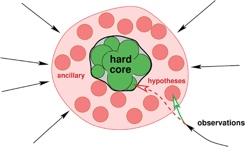
• The hard core of the research program consists of a basic theory, i.e. a set of mutually linked falsifiable hypotheses (green circles in Figure 1). By decision of the research group, this set is meant not to be attacked by possibly contradicting observations. This is, what Lakatos calls, the negative heuristics. However, attempts to disprove them are meant to be resolved using a ring of ancillary hypotheses (red circles in the ring in Figure 1) around the core which serve for its protection. Observations or experiments, aiming at falsifying elements of the hard core, also called anomalies, are “bent” toward the ancillary hypotheses, which may be falsified. The idea behind this process goes back to the thesis of Quine (1951) and Duham (1954), who observe, that “the field is so undetermined by its boundary conditions, experience, that there is much latitude of choice as to what statements to reevaluate in the light of any single contrary experience” (Quine 1951, sect. VI) and “A “Crucial Experiment” is impossible in physics” (Duham 1954, sect. 3). The boundary conditions, mentioned by Quine, may refer to both, to the precise meaning of the used concepts and to the meaning of the predicted observables, e.g. the assumption that light rays are straight, or the measurement tools are perfectly calibrated. These assumptions may be turned into ancillary hypotheses, which when confronted with contradicting observations may be augmented or changed. Each step needs to increase the power of the research program, e.g. by integrating ancillary hypotheses into the kernel, in case they resist a large number of attacks by experiments.

• The positive heuristics consists of a strategy to increase the predictive power of the research program, by giving hints on how to increase the complexity of central theory. This prevents the researcher from being irritated by a possibly large number of anomalies, but motivates him/her to concentrate on the conceptual development of the theory leading to a sequence of increasingly powerful theories. “For a theoretician the real challenges are much more mathematical difficulties than anomalies” (Lakatos 1982, sect. 3b).

The goal is to lead the research program in a progressive manner, i.e. extending the complexity of its basic theory and thus the number of possibly risky hypotheses, while simultaneously accepting its potential failure. This makes the concept a more realistic extension of Popper’s (1934) proposal that theories actually may be falsified by a single crucial experiment.

We will now dive into Ackermann’s research program and identify, due to the limitations of this format of publication, some ingredients of its hard core, its negative and its positive heuristics, especially how it evolved over time and interacted with neighboring disciplines.

3.2. Ackermann’s research program

Ackermann’s central idea is the methodological basics of theoretical accuracy evaluations of adjustment methods. We will elaborate on this methodological basis and address four aspects: (1) mathematical models, (2) theoretical precision and reliability, (3) rigorous and approximate methods, and (4) test fields.

3.2.1. Mathematical models

When transferring photogrammetric operations, such as determining the orientation of images, onto computers, the classical principles of those times, such as determining photogrammetric models,⁷ stepwise forming strips, following the flight line, and finally joining the strips to large ensembles, these processes were mimicked accepting the boundary conditions of low computation power in the 60s. No coherent theory was available embedding these individual steps. Interpreting the process of simultaneously determining the poses of the cameras during exposure, the 3D coordinates of the scene points and the parameters describing the geometric properties of the camera as proposed by Schmid (1958) were parallely picked up by Brown (1974) and Ackermann (1966).

Common to all is the idea of a mathematical model, which contains all assumptions. All observations are treated as a sample of a multidimensional distribution, in the first instance represented by its mean and its covariance matrix. Ackermann (1965, p. 9) is very clear on what observations are: “The measurements, which are used within an adjustment, primarily are just numbers, which obtain a meaning as observations only by their role within the total system of aerotriangulation,” referring to this context, which is of course to be specified before starting the measuring process.

The mathematical model consists of (1) a functional model which relates the expectation values $E(\underset{\_}{\mathit{l}})$ of all observations $\mathit{l}$ with all unknown parameters $\mathit{x}$ and (2) a stochastical model, representing the uncertainty of the observations – implicitly assuming the experiment could be repeated many times.⁸ Hence, the first two moments of the distribution are specified in the following manner

(1) $\mathrm{E}(\underset{\_}{\mathit{l}})=\mathit{f}\left(\mathit{x}\right)\mathrm{a}\mathrm{n}\mathrm{d}\mathrm{D}(\underset{\_}{\mathit{l}})={\mathrm{\Sigma }}_{ll}\mathrm{o}\mathrm{r}\underset{\_}{\mathit{l}}\sim \mathcal{N}\left(\mathit{f}(x),{\mathrm{\Sigma }}_{ll}\right).$(1)

The assumption of the normal distribution implicitly follows from (1) the optimization function $\mathrm{\Omega }=\mathit{v}{}^T{\mathrm{\Sigma }}_{ll}^{-1}\mathit{v}$, namely the weighted sum of the residuals, via the principle of maximum likelihood which essentially maximizes $\mathrm{e}{ }^{-\mathrm{\Omega }}$, or (2) from the assumption that only the first two moments of the distribution are known, using the principle of maximum entropy (Cover and Thomas 1991, Chapt. 12). If the functions $\mathit{f}$ would be linear, we would arrive at the classical (linear) Gauss – Markov model, therefore, eq. (1) describes a non-linear Gauss-Markov model. These assumption allow to estimate the best parameters $\hat{\mathit{x}}$, i.e. those minimizing their uncertainty⁹

(2) $\hat{\mathit{x}}={\hat{\mathit{x}}}^a+(A{}^T{\mathrm{\Sigma }}_{ll}A{)}^{-1}A{}^T{\mathrm{\Sigma }}_{ll}(\mathit{l}-\mathit{f}({\hat{\mathit{x}}}^a))$(2)

together with their expected or – in geodetic/photogrammetric terms theoretical precision, namely,

(3) ${\mathrm{\Sigma }}_{\hat{x}\hat{x}}=N{}^{-1}\mathrm{w}\mathrm{i}\mathrm{t}\mathrm{h}N=A{}^T{\mathrm{\Sigma }}_{ll}A\mathrm{a}\mathrm{n}\mathrm{d}A=\frac{\mathrm{\partial }\mathit{f}(\mathit{x})}{\mathrm{\partial }\mathit{x}},$(3)

where the Jacobian $A$ is to be evaluated at the estimated parameters.

Observe the non-mentioned assumptions:

• The functions $\mathit{f}$ as well the covariance matrix ${\mathrm{\Sigma }}_{ll}$ are assumed to be known.

• Following the principle of maximum entropy, assuming only the first two moments are known, implicitly postulates the distribution is a Gaussian distribution.

• No outliers are assumed.

• No constraints among the observations or between the observations and the parameters are allowed.

Of course these assumptions in reality are violated, leading to results which formally contradict the expectations. We will discuss the observed deviations in context of block adjustment and image matching.

3.2.2. Theoretical precision and reliability

Results of an estimation process may show a high theoretical precision but may still be wrong. This is because precision only reflects the sensitivity of the result with respect to random errors, which are mostly relatively small. Outliers or other errors in the functional model may deteriorate the result to a much higher degree, compared to the standard deviations of the unknown parameters. This is why Ackermann followed the concept of reliability¹⁰ according to Baarda (1967, 1968). This is an example of how he augmented the original meaning of the central theory, specifically the model (1) which assumes a Gaussian distribution, in case reality attacks it, here by outlying observations.

3.2.3. Rigorous and approximate methods

From the beginning, Ackermann aimed at developing rigorous methods. A method is called rigorous, if all its components are consistent, i.e. if all components of the mathematical model are used during the optimization.¹¹

The value of rigorous methods is that their properties are more likely to be understood, than non-rigorous, or approximate methods.

As an example, bundle adjustment is rigorous if the functional model reflects the collinearity equations, all image coordinates are assumed to have the same standard deviation, no outliers exist, and the reprojection error is minimized using iterative least squares.

This may be an approximate solution. As an example, assume the measured image points have individual covariance matrices, since then the individual variances and the correlations between the $x$- and $y$-coordinates are neglected when minimizing the reprojection errors.

An essential part of the research program was, to identify such approximations, to establish corresponding ancillary hypotheses, with the goal of integrating them into the hard core of the theory, by showing their resistance to experimental attacks, i.e. that the extended theory cannot be disproved by experiments.

3.2.4. Checking the theory

Checking the theory therefore played a central role within the research program. They were based on test fields using costly state-of-the-art methods. The essence of the design of these test fields was to evaluate various kinds of modifications of the basic theory, especially allowing to check changes in functional or the stochastical model. This not only referred to the assumed standard deviations of the observations but also to their correlations. As an example (Stark 1973) investigated the causes and effects of correlations between image coordinates of points within an image and addressed the aspect of exchanging refinements of the functional and the stochastical model.

The motivation for these test fields was both scientifically and practically. On the one hand, the development of the theory was extremely rapid, which required an immediate check on its new components – as a researcher one is always (at least should be) skeptical w.r.t. the own progress. On the other hand, the methods had practical implications, allowing to replace traditional methods: this required careful, sincere, and transparent investigations in order to be able to convince practitioners – which not always was successful.

4. Block adjustment

Block adjustment aims to simultaneously (en bloc, fr.) estimate the transformation parameters of a set of units and the coordinates of scene points from observed points in the units. We will discuss the concept and the experiments for checking the theory.

4.1. Concept of block adjustment

The units of a block adjustment are images or photogrammetric models, and the observed points in the scene and the units are 2D or 3D points with their 2D- or 3D-coordinates. This results in at least three basic problems, collected in Table 1, together with their extensions, taken from (Förstner and Wrobel 2016, p. 649).

Table 1. Types of block adjustments. BA $=$ bundle adjustment: observations are bundles of rays: MA $=$ model block adjustment; observations are model points; $D_I$ $=$ dimension of scene points; $D_T$ $=$ number of transformation parameters per unit; $D_E$ $=$ dimension of observables; PH $=$ photogrammetry; CV $=$ computer vision.

	Name	Scene feature	Transformation	Observations	Main application
1	BA	3D points	Projective transformation/	Image points	PH/CV
			3D motion
		$D_I=3$	$D_T=11/6$	$D_E=2$
2	3D MA	3D points	3D homography/	local	PH/CV
			3D similarity/	3D points
			3D motion
		$D_I=3$	$D_T=15/7/6$	$D_E=3$
3	2D MA	2D points	2D homography/	2D points	Photography/
			2D similarity/		PH/CV/
			2D motion		Robotics
		$D_I=2$	$D_T=8/4/3$	$D_E=2$

When Ackermann started his research in Stuttgart at the newly established Institute for Photogrammetry, among the eight variations mentioned in the table, only three were in focus:

1. Bundle adjustment, starting from image points and aiming at the 3D motion of the cameras. This setup was seen as the most rigorous approach for handling images.

2. 3D block adjustment, starting from the 3D coordinates of photogrammetric models and aiming at their 3D motion. This setup reflected the current way of first (analogously) establishing stereo models, measuring 3D point in a stereo instrument, and then performing the pose estimation by computer.

3. 2D block adjustment, starting from the 2D planar coordinates of (leveled) photogrammetric models and aiming at their 2D similarity. This setup was of great advantage, as it significantly reduced the number of unknown parameters per photogrammetric model from 6 to 4, and – most significantly – provided a direct solution, i.e. not requiring approximate values. At the same time, the method was an excellent tool to determine approximate values for bundle adjustment and 3D block adjustment, since the four parameters per photogrammetric model correspond to the 3D coordinates of the projection center and the azimuth of the image.

All three basic methods had been realized in program packages, namely for planimetric block adjustment PAT-M4, for spatial block adjustment PAT-M43,¹² and for bundle adjustment PAT-B.

Table 1 demonstrates the progressive development of the research program: In all three cases the transformations were later exchanged by more general or specific ones reflecting the geometrical of physical boundary conditions.

The existence of three partially competing methods was the basis for intensive theoretical and practical studies.

For example, at the ISP symposium 1976 in Stuttgart, the results using benchmark data seemed to suggest that the method of 3D block adjustment leads to more accurate results than those using bundle adjustment. This clearly contradicted the theoretical expectations: Since 3D block adjustment starts from 3D coordinates of photogrammetric models, the measured 3D points are highly correlated, due to (1) random errors in the relative orientation of the image pairs and (2) overlap of neighboring photogrammetric models. These correlations were neglected, which is why the method was also called the method of independent models. Hence, it should lead to less accurate result than the rigorous bundle adjustment method. This is an example of the positive heuristics of the research program, that the theoretical expectations were relied on, and the cause for the discrepancy between theory and experiment was identified: Systematic errors, mainly caused by lens and film distortion, were partly compensated by the generation of photogrammetric models, but were not taken into account by the bundle adjustment. This then led to the necessary extension of the functional model to characterize systematic errors using additional parameters.

4.1.1. Additional parameters

Simple bundle adjustment assumes the image points are strictly related to the scene points by the collinearity relation, formally we have $\mathrm{E}(\underset{\_}{\mathit{l}})=\mathit{f}{}^{(0)}(\mathit{t},\mathit{k})$, where the camera parameters are $\mathit{t}$ and the scene coordinates $\mathit{k}$. Therefore, in practice, the observations are generally corrected for systematic errors $\mathit{s}$, leading to the model $\mathrm{E}(\underset{\_}{\mathit{l}})-\mathit{s}=\mathit{f}{}^{(0)}(\mathit{t},\mathit{k})$. If the corrections are parametrized, e.g. by $\mathit{s}:=\mathit{s}(\mathit{p})$, we arrive at the model for bundle adjustment with additional parameters, or selfcalibrating bundle adjustment

(4) $\mathrm{E}(\underset{\_}{\mathit{l}})=\mathit{f}(\mathit{t},\mathit{k},\mathit{p}).$(4)

Hence, augmenting the set of unknown parameters leads to a more powerful model for bundle adjustment. Again, this augmentation easily can be identified as a hypothesis motivated by the positive heuristics of the research program.

However, it is by no means clear how to parameterize the corrections, which actually are meant to model the complex process of taking an (analog) image with a real camera. Schilcher (1980) mentions around 50 different physical reasons which influence image coordinates, most having similar effects. Kilpelä (1980) summarizes the attempts to parametrically model systematic errors and cites 14 different proposals. It is interesting to identify two views on how to choose a correction model:

1. A physical view. Prominent representative is D. Brown’s (1966, 1971) attempt to model the physics of lens distortion and the effect of film flatness.

2. A phenomenological view. Prominent representative is Ebner’s (1976) proposal to choose orthogonal polynomials, since additional parameters are treated as nuisance parameters within the bundle adjustment and have no value for themselves.

Of course all authors, presenting a new parametrization of systematic errors, had individual arguments. However, due to the limited number of additional terms and the impossibility to truly map reality into mathematical terms, none of them turned out to be superior over all others in the long run. The limitation in complexity was partly overcome by using splines, e.g. Rosebrock and Wahl (2012) with nearly 100 parameters or even Schops et al. (2020),¹³ who work with a $50\times 50$ grid for the spline corrections in both coordinates or Fourier series (Tang, Fritsch, and Cramer 2012).

The question on whether to follow a physical or a phenomenological view in the 70s is the same as the recent discussion on the modeling of features for image interpretation using neural networks: Here often millions of parameters are learnt (estimated) from training data for adapting to the complexity of the image structures and avoid the otherwise necessary engineering task of designing appropriate image features for object recognition.

4.1.2. Control information and ancillary observations

Images alone only provide 3D information up to a spatial similarity transformation. Control points, i.e. 3D scene points with known coordinates, were required for geometric scene reconstruction from the beginning. Without using the power of the basic theory of block adjustment, the number of control points increased proportional to the area of the covered region and for small-scale applications in unknown areas the determination of the coordinates of the control points was costly. The exploitation of the statistically rigorous estimation method, realized in block adjustment, had two essential consequences:

1. For planimetry, the number of required control points only increased proportional to the perimeter of the covered region. This led to the recommendation to increase the block size. Large blocks (Ebner, Krack, and Schubert 1977), with up to 10 000 images, were processed with the necessary development of software which could handle these cases – a positive side effect of the theoretical research: Meissl (1972) proved that the expected precision of large blocks with control points at the perimeter decreases extremely slow, namely the standard deviation of the scene point coordinates increases with the logarithm of the diameter of the area, which confirmed the findings of Ebner, Krack, and Schubert (1977), generated by explicitly inverting the normal equations for estimating the pose parameters of the entities in the block.

2. For reducing the vertical control points in the interior of the covered areas. Following early ideas of his coworkers Ackermann, Ebner and Klein (1972) identified several essential remedies which can easily be integrated into the estimation process using ancillary observations or additional parameters: (1) the use of altimeter data, i.e. observed distances from the airplane to the ground, (2) the very low curvature of the isobaric surface, and (3) shorelines of lakes, enforcing the same height. With the upcoming ability to use GPS, investigations soon showed that differential GPS can be used to determine the position of the airplane during flight with an accuracy below 10 cm, again easily integrated into the mathematical model of bundle adjustment.

4.2. Checking the theory

The role of mathematical models in our context is clarified in Ackermann’s (1965, p. 9–10) thesis: “The mathematical model, which is used for solving a specific technical task … can be chosen arbitrarily and is part of the free choice of the engineer. The choice of a specific mathematical model only depends on its practical utility.”

Theories or hypotheses, following the negative heuristics, never can be verified. We usually say the theory is verified in case a large enough number of experiments were unsuccessful making the theory/hypotheses fail.

Experiments are therefore indispensable. They are designed to identify the limitations of the research program. They serve two purposes:

1. They need to be checked w.r.t. to their predictive power.

Users are generally skeptical against new methods. Empirical studies, especially if initiated by users of the proposed methods, can then be used to identify the ability of the theory to be applicable in practical situations. The (conservative) users (implicitly) hope that the proposed method does not work properly, which indicates that these experiments are meant as attacks aiming at the failure of the research program.

2. They are needed to check the progressiveness of the research program.

Benchmarks are the classical representative for this kind of experiment. They are used to identify the effect of various modifications within the basic theory, namely (1) change of number and type of observations, e.g. by modifying the overlap of the images, (2) choice and changes of the functional model, e.g. by additional parameters or a simplified relation between observations and unknown parameters, and (3) choice and changes of the stochastical model, e.g. by neglecting variations of the standard deviations of the observations or their mutual correlations, or – when using robust methods – their ability to handle outliers.

The limitations are then used to follow the progressive heuristics and modify the hypotheses adequately. On the other hand, the empirical results of the benchmarks give clear practical hints on choosing – possibly suboptimal – methods when planning measurements.

F. Ackermann, in the early 70s, managed two benchmarks – following the investigations by Jerie (1957) in the late 60s. In all cases, photogrammetrically determined scene coordinates were compared to the geodetically determined ground truth:

(a) The test field Oberschwaben (Haug 1980), initiated in 1967/68 by the OEEPE,¹⁴ aimed at investigating the usefulness of photogrammetric block adjustment for large-scale mapping with a planimetric target accuracy of 30 cm using an image scale of 1:28 000. Ackermann’s lectures on the practical usefulness of block adjustment motivated the author to follow his proposal to investigate the limitations for very small large image scales, down to 1:500 (Förstner and Gönnenwein 1972).

(b) The testfield Appenweier (Ackermann 1974), initiated in 1973 by the Survey Department of Baden-Württemberg, aimed at identifying the potential of photogrammetric block adjustment for geodetic network densification with a planimetric target accuracy of 3 cm using an image scale of 1:7 800.

The benchmarks Appenweier and Oberschwaben had a strong influence (1) onto the photogrammetric community especially concerning the role of additional parameters and the mutual dependency of the functional and the stochastical model, but also (2) onto the rather conservative land surveyors community, who were confronted with a full-grown alternative method for the densification of geodetic networks. The 70s and 80s were sometimes perceived as the golden age of photogrammetry, with aerotriangulation as its principle topic.

5. Image matching

With Ackermann’s research proposal “Correlation of small image patches” at the German Science Foundation in 1980 a new chapter opened in the application of the research program. Since Ackermann’s scope that time was geometric image analysis and digital image interpretation using pattern recognition methods was mainly applied to remote sensing images, it was just the right time to address the use of digital images, actually digitized analog images, for geometric purposes.

5.1. Least squares matching

The conceptual challenge of deriving geometric information from digital images lies in the discrete nature of the image grid. Matching two image patches using correlation inherently refers to the grid, and enforces a final interpolation of the correlation function to find the maximum, for determining the optimal shift between the two image patches, though studies into the theoretical precision used a continuous image model (Svedlow, McGillem, and Anuta 1976).

Replacing the maximization of the empirical cross-correlation function between the two image patches by a minimization of the intensity differences in a least squares manner leads to what is called least squares matching (LSM). It was already implemented by Helava (1978); but he rejected the approach for a simple practical reason: too accurate approximate values are necessary and did not publish any details. This development occurred independent of the work of B. Lucas’ PhD Lucas (1984); Lucas and Kanade (1981).

Wild (1983), a PhD student of Ackermann working in the area of interpolation with weight functions,¹⁵ proposed to take a continuous view, reconstructing the hidden continuous image from the discrete grid values and integrating a geometric and radiometric transformation between the two images. Estimating the eight parameters (six for geometry, two for radiometry) led to the desired matching between the two image patches.

So, with the two image grids $f(\mathit{x})$ and $g(\mathit{y})$ and the unknown parameters ${\mathit{p}}_G$ and ${\mathit{p}}_R$ for the affine geometric and the radiometric transformations $T_G$ and $T_R$, the functional model for the $k$-th pixel $g({\mathit{y}}_k)$ in the second image is (Förstner 1993) as follows:

(5) $\mathrm{E}(\underset{\_}{g}({\mathit{y}}_k))=T_r\left\{f\left[T_G\left(\mathit{x};\mathit{p}{}_G\right);p_R\right]\right\}\mathrm{w}\mathrm{i}\mathrm{t}\mathrm{h}k=1,\dots ,K.$(5)

The model is fully consistent with the basic model (1) of the core of the research program. The matching model appears limited, since

• the function $f$, as template, needs to be known completely,

• only the second grid $g({\mathit{y}}_k)$, with its $K$ pixels, is assumed to be observed,

• assuming all intensities have the same accuracy,

• requiring good approximate values – looking into the future –

• only two image patches are involved, and

• the patches have limited size, in order to approximately fulfill the geometric model, an affinity.

All these deficiencies were addressed – partly much later – without reference here.

Wild’s idea initially was realized using inverse quadratic radial basis functions, which were soon replaced by bilinear interpolation, which highly increased efficiency (Ackermann 1984). In spite of the mentioned limitations, investigations into the theoretical accuracy of the method showed the enormous potential of the method, being able to reach translation accuracies of below 1/50 pixel (Förstner 1982) and its dependency on image filtering. This kept the motivation to proceed this line of thought alive, again an indication of the strong positive heuristics of the research program. Ackermann, when confronted with these results, said: If this is true, this is a break-through. Make sure, this actually holds. Nobody should be able to disgrace us. The predicted precision was confirmed experimentally, e.g. in the master thesis of Vosselman (1986) and found wide acceptance, especially in close range photogrammetry for high precision surface reconstruction (Schewe 1988; Schneider 1990)

5.2. Feature-based image matching and automatic DEM generation

The main remedy against the broad practical use of least squares image matching is the small radius of convergence. Following the idea of Barbard and Thomson (1980), a method for solving the problem of image matching by using image features, namely keypoints, was developed following the concept of the basic research program: (1) detecting keypoints based on the expected theoretical precision of LS, (2) establishing a list of putative correspondences based on the correlation coefficient, and (3) determining the mutual geometric transformation by a robust estimation procedure Paderes, Mikhail, and Förstner (1984); Förstner (1986). If the image patches overlap up to 50%, the method can handle large image patches without requiring approximate values. The accuracy of the resulting transformation is generally good enough that a subsequent LSM at the final matches can converge.

The approach was integrated into an automatic method for generating digital elevation models (DEM) from completely digital aerial image, using image pyramids (Ackermann and Hahn 1991) realized in the program package Match–T (Krzystek 1991). It is interesting to observe, that this method does not use least squares matching: A huge number of 3D points of medium accuracy leads to a sufficiently accurate DEM.

6. Closing

We discussed some aspects of the historical development of the research program of Friedrich Ackermann. It is only a rough sketch, omitting various achievements, due to the scale of this paper: a few pages compared with 26 PhD’s and more than 100 scientific papers. Especially, we did not touch his later work on GIS, education, and the role of photogrammetry in general. We also focused on his research, and gave only a glimpse into his achievements transferring his knowledge and experiences into the world of mapping and geoscience via courses and software, which are comparably profound.

When discussing the future of photogrammetry which lay and still lies in the area of image interpretation Ackermann always had his basic concept of observations within a theory in mind: he did not agree with the terms information extraction or feature extraction from images, since digital images are just large collections of numbers, which obtain their meaning from the concept how they are evaluated, geometrically or thematically. In this respect, he followed the school of constructivism, which starts with the assumption that objects and meanings are constructed by the observer – man or machine – a view which puts the burden of evaluating images onto the modeling capabilities of the engineer – including his/hers responsibility for choosing adequate models. Approaches of pattern recognition, machine learning, and artificial intelligence follow this line, since the relation between the raw data (digital images) and the derived interpretations is provided by the possibly annotated data sets and the chosen classification scheme.

On the one hand, the core of Ackermann’s research program, the statistical estimation theory, with its probabilistic basis, will further show a positive development. As an example, the research program was picked up by the Computer Vision community, see the extensive review by Triggs et al. (2000). Today, in Computer Vision, the notion bundle adjustment often is used in the meaning of simultaneously estimating the parameters of all units at the same time – implicitly referring to the original notion of en bloc-adjustment. The research program certainly will play a central role, especially if image interpretation is modeled probabilistically.

On the other side, statistical models in image analysis and image interpretation are under attack: Neither the distribution of digital images nor the uncertainty of the estimated parameters – in a neural network – can be really handled due to the enormous probability spaces with myriads of dimensions, only $2^{{10}^4}\approx {10}^{300}$ for a small 100$\times$100 binary image, which cannot be filled with enough data to be able to reasonably estimate densities. Therefore, (1) the effect of only simplified versions of the uncertainty of the trained models can be tracked to the resulting interpretation results by Monte Carlo techniques, and (2) it prevents the exploitation of classical shortcuts for predicting the quality of results, given a mathematical model and a certain observation design. Benchmarks then have a different, and much more important and practical role: They are not used to check the predictions of a theory, but to demonstrate the usefulness of a given method, which, in spite of the huge size of the training data in a learning scenario, but due to unknown model uncertainties, can very well be doubted – at least be discussed.

The author is grateful for the many discussions with Friedrich Ackermann on conceptual problems in our specific engineering discipline. Ackermann shaped the research in its transition from analog, via analytical to digital photogrammetry. He always set high scientific goals in a self-critical habit. His basic attitude was to integrate, basic and applied science with motivating education, gave courage to approach new shores of insights while as supervisor gave the freedom to find ones own way.

Additional information

Notes on contributors

Wolfgang Förstner

Wolfgang Förstner, studied Geodesy at Stuttgart University where he also finished his PhD. From 1990-2012 he chaired the Department of Photogrammetry at Bonn University. His fields of interest are digital photogrammetry, statistical methods of image analysis, analysis of image sequences, semantic modelling, machine learning and geo information systems. He published more than 200 scientific papers, supervised more than 100 Bachelor and Master Theses and supervised 34 PhD Theses. He served as associated editor of IEEE Transactions on Pattern Analysis and Machine Intelligence. He obtained the Photogrammetric (Fairchild) Award of American Society of Photogrammetry and Remote Sensing 2005, honorary doctorates from the Technical University of Graz and the Leibniz University of Hannover, 2016 the Brock Gold Medal Award of the International Society of Photogrammetry and Remote Sensing (ISPRS) and 2020 the ISPRS Karl Kraus Medal for the textbook on ‘Photogrammetric Computer Vision’.

Notes

1. This refers to the expected precision of the estimated quantities derived from the Cramer-Rao bound, namely the inverse of the normal equation matrix.

2. This is closely related to sparse image sequences.

3. The term triangulation is borrowed from geodetic networks.

4. This is the geodesy internal naming of statistical estimation theory.

5. The term “block” is taken from the French “en bloc”, referring to the simultaneous determination of all unknown entities.

6. Photogrammetry in the wide sense aims at deriving information from images. Both focus on applications in surveying, mapping and high-precision metrology, Ikeuchi (2014, Chapt. Photogrammetry).

7. These are pairs of overlapping images, which were the basis for 3D mapping, and in a first step consisted of a set of 3D points and the projection centers of the two images involved. Sometimes only the xy-coordinates of the 3D points were used after enforcing the model to be leveled.

8. Originally, following the Delft School of geodesy, the functional model was named mathematical model which had an associated stochastical model, expressing the idea that both models can be changed without changing the other. We prefer to see the two models, referring to the functions and the stochastical properties as part of a joint view, since the stochastical model explicitly refers to the parameters of the functional model.

9. These are locally best linear unbiased estimates.

10. The notion “reliability” here is coherent with Huber’s (1991) notion of “diagnostics”.

11. Observe, the attribute rigorous and the attribute acceptable are independent. If a method is rigorous, this does not tell whether it is acceptable for a certain application or not. On the other side, a non-rigorous method may be acceptable.

12. The abbreviation “43” indicates, that the adjustment was performed by iterating planimetric with four parameters per unit and height blocks with three parameters per unit.

13. The title refers back to the number 12 of Ebner’s (1976) additional parameters.

14. Organisation Europeenne d’Etudes Photogrammetriques Experimentales – today European Spatial Data Research (EuroSDR).

15. Weight functions actually are kernel functions.

References

- Ackermann, F. 1965. Fehlertheoretische Untersuchungen über die Genauigkeit photogrammetrischer Streifentriangulationen. Reihe C 87. München: Deutsche Geodätische Kommission bei der Bayerischen Akademie der Wissensch.
- Ackermann, F. 1966. “On the Theoretical Accuracy of Planimetric Block Triangulation.” Photogrammetria 21 (5): 145–170. https://doi.org/10.1016/0031-8663(66)90009-3.
- Ackermann, F. 1974. “Photogrammetric Densification of Trigonometric Networks – The Project Appenweier.” Bildmessung und Luftbildwesen 6:189–192.
- Ackermann, F. 1984. “Digital Image Correlation: Performance and Potential Application in Photogrammetry.” Photogrammetric Record 11 (64): 429–439. https://doi.org/10.1111/j.1477-9730.1984.tb00505.x.
- Ackermann, F., H. Ebner, and H. Klein. 1972. “Combined Block Adjustment of APR Data and Independent Photogrammetric Models.” The Canadian Surveyor 26 (4): 384–396. https://doi.org/10.1139/tcs-1972-0063.
- Ackermann, F., and M. Hahn. 1991. “Image Pyramids for Digital Photogrammetry.” In Digital Photogrammetric Systems, edited by H. Ebner, D. Fritsch, and C. Heipke, 43–58. Berlin: Wichmann-Verlag.
- Baarda, W. 1967. Statistical Concepts in Geodesy. Vol. 2/4 of Publication on Geodesy, New Series. Delft, The Netherlands: Netherlands Geodetic Commission. https://doi.org/10.54419/bjdeu2.
- Baarda, W. 1968. A Testing Procedure for Use in Geodetic Networks. Vol. 2/5 of Publication on Geodesy, New Series. Delft, The Netherlands: Netherlands Geodetic Commission. https://doi.org/10.54419/t8w4sg.
- Barbard, S. T., and W. B. Thomson. 1980. “Disparity Analysis of Imges.” IEEE Transactions on Pattern Analysis & Machine Intelligence 2 (4): 333–340. https://doi.org/10.1109/TPAMI.1980.4767032.
- Brown, D. C. 1966. “Decentering Distortion of Lenses.” Photogrammetric Engineering 32 (3): 444–462.
- Brown, D. C. 1971. “Close-Range Camera Calibration.” Photogrammetric Engineering 37 (8): 855–866.
- Brown, D. C. 1974. “Bundle Adjustment with Strip- and Block-Invariant Parameters.” Bildmessung und Luftbildwesen 44:128–139.
- Cover, T. M., and J. A. Thomas. 1991. Elements of Information Theory. Hoboken, New Jersey: John Wiley & Sons. https://doi.org/10.1002/0471200611.
- Duham, P. 1954. “Physical Theory and Experiment.” In Philosophy of Science: The Central Issues, 1998, edited by M. Curd and J. A. Cover. New York, USA: W. W. Norton and Company.
- Ebner, H. 1976. “Self Calibrating Block Adjustment.” Zeitschrift für Bildmessung und Luftbildwesen 44:128–139.
- Ebner, H., K. Krack, and E. Schubert. 1977. “Genauigkeitsmodelle für die Bündelblocktriangulation.” Bildmessung und Luftbildwesen 5:141–148.
- Förstner, W. 1982. “On the Geometric Precision of Digital Correlation.” In Intl. Archives of Photogrammetry, edited by J. Hakkarainen, E. Kilpelä, and A. Savolainen, 176–189. Vols. XXIV–3, Jun. Helsinki: ISPRS Symposium, Comm. III.
- Förstner, W. 1986. “A Feature Based Correspondence Algorithm for Image Matching.” In Intl. Archives of Photogrammetry and Remote Sensing, edited by E. Kilpelä, 150–166. Vol. 26, Part 3/3. Rovaniemi, Finland: ISP Symposium, Comm. III.
- Förstner, W. 1993. “Image Matching.“ In Computer and Robot Vision. Vol. II, Chap. 16, 289–379. Boston, USA: Addison Wesley.
- Förstner, W., and H. Gönnenwein. 1972. “Photogrammetrische Punktbestimmung aus extrem gro ma stäbigen Bildern - Der Versuch Böhmenkirch.” Allgemeine Vermessungs – Nachrichten 7: 271–291.
- Förstner, W., and B. P. Wrobel. 2016. Photogrammetric Computer Vision – Statistics, Geometry, Orientation and Reconstruction. Springer International Publishing. https://doi.org/10.1007/978-3-319-11550-4.
- Haug, G. 1980. Bestimmung und Korrektur systematischer Bildund Modelldeformationen der Aerotriangulation am Beispiel des Testfeldes “Oberschwaben”. Frankfurt/M, Germany: Institut für Angewandte Geodäsie, Publication of Organisation Europeenne d’Etudes Photogrammetriques Experimentales.
- Helava, U. V. 1978. “Digital Correlation in Photogrammetric Instruments.” Photogrammetria 34 (1): 19–41. https://doi.org/10.1016/0031-8663(78)90020-0.
- Huber, P. J. 1991. “Between Robustness and Diagnostics.” In Directions in Robust Statistics and Diagnostics, edited by W. Stahel and S. Weisberg, 121–130. New York, Berlin, Heidelberg, London, Paris, Tokyo, Hong Kong, Barcelona: Springer.
- Ikeuchi, K., edited by. 2014. Computer Vision – A Reference Guide. Springer US. https://doi.org/10.1007/978-0-387-31439-6.
- Jerie, H. G. 1957. “Block Adjustment by Means of Analogue Computers.” Photogrammetria 14:161–176. https://doi.org/10.1016/S0031–866(3()57)80022–2.
- Kilpelä, E. 1980. “Compensation of Systematic Errors of Image and Model Coordinates.” In Intl. Archives of Photogrammetry and Remote Sensing, edited by G. Konecny and G. Böttcher, 407–427. Vol. XXIII. Hamburg: Proc. XIVth ISPRS Congress.
- Krzystek, P. 1991. “Fully Automatic Measurement of Digital Elevation Models with MATCH–T.” In Photogrammetric Week, Schriftenreihe, Institute of Photogrammetry, edited by F. Ackermann and D. Hobbie, 203–214. Vol. 15. Stuttgart, Germany: Stuttgart University.
- Lakatos, I. 1982. Die Methodologie der wissenschaftlichen Forschungsprogramme. Braunschweig, Germany: Vieweg. https://doi.org/10.1007/978-3-663-08082-4.
- Lucas, B. D. 1984. “Generalized Image Matching by the Method of Differences.” PhD diss., Pittsburgh: CarnegieMellon University, Computer Science Department.
- Lucas, B. D., and T. Kanade. 1981. “An Iterative Image Registration Technique with an Application to Stereo Vision.” In International Joint Conference on Artificial Intelligence, B.C., Canada, 674–679.
- Meissl, P. 1972. “A Theoretical Random Error Propagation Law for Anblock-Networks with Constrained Boundary.” Österreichische Zeitschrift für Vermessungswesen 60:61–65.
- Paderes, F. C., E. M. Mikhail, and W. Förstner. 1984. “Rectification of Single and Multiple Frames of Satellite Scanner Imagery Using Points and Edges as Control.” In Proc. of the 2nd Annual NASA Symposium on Mathematical Pattern Recognition & Image Analysis, edited by L. F. Guseman, College Station, TX 77843, NASA Johnson Space Center, Texas A & M University, july 92.
- Popper, K. 1934. Logik der Forschung. 4th ed. Mohr Siebeck, Tübingen. https://doi.org/10.1007/978-3-7091-4177-9.
- Quine, W. V. O. 1951. “Two Dogmas of Empiricism.” The Philosophical Review 60 (1): 20–43. https://doi.org/10.2307/2181906.
- Rosebrock, D., and F. M. Wahl. 2012. “Generic Camera Calibration and Modeling Using Spline Surfaces.” 2012 IEEE Intelligent Vehicles Symposium, Alcala de Henares, Spain, 51–56.
- Schewe, H. 1988. Automatische photogrammetrische Erfassung von Industrieoberflächen. Technical Report. Stuttgart: Inpho GmbH.
- Schilcher, M. 1980. Empirisch-statistische Untersuchungen zur Genauigkeitsstruktur des photogrammetrischen Luftbildes. Reihe C 262. München: Deutsche Geodätische Kommission bei der Bayerischen Akademie der Wissenschaften.
- Schmid, H. H. 1958. “Eine allgemeine analytische Lösung für die Aufgabe der Photogrammetrie.” Bildmessung und Luftbildwesen 26/27 (11/12): 103–113, 1959:1–12.
- Schneider, C.-T. 1990. Objektgestützte Mehrbildzuordnung. Reihe C 375. Munich, Germany: Deutsche Geodätische Kommission bei der Bayerischen Akademie der Wissenschaften.
- Schops, T., V. Larsson, M. Pollefeys, and T. Sattler. 2020. “Why Having 10,000 Parameters in Your Camera Model is Better Than Twelve.” In 2020 IEEE/CVF Conference on Computer Vision and Pattern Recognition (CVPR), 2532–2541. Los Alamitos, CA, USA: IEEE Computer Society, june
- Stark, E. 1973. Die Genauigkeitsstruktur im photogrammetrischen Einzelmodell. Dissertationen Reihe C 193. Munich, Germany: Verlag der Bayr. Akademie der Wissenschaften, Deutsche Geodätische Kommission.
- Svedlow, M., C. D. McGillem, and P. Anuta. 1976. Analytical and Experimental Design and Analysis of an Optimal Processor for Image Registration. Technical Report Inf. Note 090776. West Lafayette: LARS, Purdue Univ.
- Tang, R., D. Fritsch, and M. Cramer. 2012. “New Rigorous and Flexible Fourier Self-Calibration Models for Airborne Camera Calibration.” ISPRS Journal of Photogrammetry and Remote Sensing 71:76–85. https://doi.org/10.1016/j.isprsjprs.2012.05.004.
- Triggs, B., P. McLauchlan, R. Hartley, and A. Fitzgibbon. 2000. “Bundle Adjustment — A Modern Synthesis.” In Vision Algorithms: Theory and Practice, edited by B. Triggs, A. Zisserman, and R. Szeliski, 298–372. Vol. 1883 of LNCS, 298372. 298372. Proc. of the Intl. Workshop on Vision Algorithms: Theory and Practice. Springer. https://doi.org/10.1007/3-540-44480-7_21.
- Vosselman, G. 1986. “An investigation into the precision of a digital camera.” Master’s thesis, Technical University of Delft.
- Wild, E. 1983. Die Prädiktion mit Gewichtsfunktionen und deren Anwendung zur Beschreibung von Geländeflächen bei topographischen Geländeaufnahmen. Reihe C 277. Munich, Germany: Deutsche Geodätische Kommission.