Wave retrieval from quad-polarized Chinese Gaofen-3 SAR image using an improved tilt modulation transfer function

ABSTRACT

An accurate Modulation Transfer Function (MTF) is essential for Synthetic Aperture Radar (SAR) wave spectra retrieval. This study aimed to investigate the performance of a quad-polarized wave retrieval algorithm based on fully polarimetric SAR image data using the improved tilt MTF and considering the influence of wind speed. The tilt MTF is the key factor in the wave retrieval scheme from quad-polarized (Vertical–Vertical (VV), Horizontal–Horizontal (HH), Vertical–Horizontal (VH), and Horizontal–Vertical (HV)) SAR images. In this study, the waves were inverted from more than 1300 Gaofen-3 (GF-3) images acquired in quad-polarization strip mode with a spatial resolution of 16 m and a swath coverage of 50 km. The winds were retrieved using the Geophysical Model Function (GMF) C-band SAR model for Gaofen-3 (CSARMOD-GF), which is suitable for re-calibrated GF-3 images in VV-polarization. The comparison of the wind speed yielded a Root Mean Square Error (RMSE) of 1.73 m/s and a Correlation Coefficient (COR) of 0.94. The validation of the Significant Wave Height (SWH) simulated using the Waves Nearshore (SWAN) model against Haiyang-2B (HY-2B) altimeter data yielded an RMSE of 0.56 m and a COR of 0.87. The results reveal that the SAR-derived wind and SWAN-simulated SWH are suitable for analysis of SAR wave retrieval. The full polarimetric technique was applied to the collected images, and the statistical analysis yielded a RMSE of 0.51 m, a COR of 0.75, and a Scatter Index (SI) of 0.44 compared with the SWHs retrieved using the simulations from the SWAN model. The non-polarized contribution in the Normalized Radar Cross Section (NRCS; unit: dB) caused by wave breaking ${\sigma }_0^{wb}$ was calculated using a theoretical approach that employs the VV-polarized calibrated NRCS ${\sigma }_0^{\mathrm{v}\mathrm{v}}$ and HH-polarized calibrated NRCS. The effect of wave breaking on the SAR retrieval waves was studied. The bias (SAR-derived minus SWAN-simulated SWH) increased as the (${\sigma }_0^{wb}$/${\sigma }_0^{\mathrm{v}\mathrm{v}}$) ratio (>0.4) increased, and the accuracy improved when the ratio was less than 0.4. This behavior is reasonable since the wave breaking inevitably affects the tilt modulation. Therefore, wave breaking should be considered in SAR wave retrieval using the approach proposed in this paper under extreme sea states, such as typhoons and hurricanes.

KEYWORDS:

• Wave retrieval
• Gaofen-3 (GF-3)
• Synthetic Aperture Radar (SAR)

1. Introduction

Traditionally, sea surface waves, which play an essential role in momentum and heat exchanges at the air–sea interface and interact with mesoscale marine phenomena, are measured using moored buoys in real time (Steele, Lau, and Hsu 1985). Based on the development of wave theory and computer technology, the waves are hindcast simulated using a numerical wave model, i.e. the Simulating Waves Nearshore (SWAN) model (Sun, Perrie, and Toulany 2018) and the WAVEWATCH-III model (Tolman and Booij 1998). The numerical model is applicable under extreme sea states (Sheng et al. 2019; Yang et al. 2020); however, the accuracy and spatial resolution of the wave modeling rely on the forcing field. Since the 1990s, remote sensing has continuously provided data on the sea surface dynamics over the global seas, which have been commonly used in oceanography research.

Compared with existing remote-sensing techniques, i.e. scatterometers (i.e. 0.25° grid spatial resolution) (Isaksen and Stoffelen 2000) and altimeters (i.e. a spatial resolution of 10 km following the satellite footprint) (Zhang et al. 2003), Synthetic Aperture Radar (SAR) has good capability for sea surface wind and wave monitoring with a fine spatial resolution and wide coverage, especially under oil-slick (Jiang et al. 2023), Tropical Cyclone (TC) (Shao et al. 2020), and Arctic Ocean conditions (Shao et al. 2022). As revealed in the SeaSAT mission prompted by the National Aeronautics and Space Administration, the co-polarized (Vertical–Vertical (VV) and Horizontal–Horizontal (HH)) SAR backscattering signal represented by the Normalized Radar Cross Section (NRCS) is linearly correlated with the wind speed (Masuko et al. 1986), which is consistent with the findings from scatterometer observations. Following this rationale, Geophysical Model Functions (GMFs) that were empirically designed for scatterometer wind retrieval, i.e. C-band Model 4 (CMOD4) (Stoffelen and Anderson 1997) and CMOD-IFR (Quilfen et al. 1998), have been applied to SAR data due to the sufficient SAR measurement dataset. Subsequently, the C-band Model (CMOD) was further improved, and updated versions have been gradually released, i.e. CMOD5 (Hersbach, Stoffelen, and Haan 2007) and CMOD7 (Stoffelen et al. 2017). Although the wind data retrieved from SAR data using scatterometer-based GMFs is reliable (Monaldo et al. 2016; Shao et al. 2014), the dependence of other marine phenomena at the mesoscale is exclusive in a GMF, resulting in distortion of the SAR wind retrieval under complicated sea states (Xu et al. 2018). In recent studies, two approaches have been proposed to solve this problem, i.e. the improvement of a GMF using SAR-measured NRCS (Lu et al. 2018) and an analytical retrieval model that accounts for the influences of wave-current interactions and wave breaking (Yao et al. 2022). Currently, SAR-based GMFs for the C-band have been well developed under low-to-moderate wind conditions, i.e. C-band SAR Model (C-SARMOD) for Sentinel-1 (S-1) (Mouche and Chapron 2016) and C-band SAR Model (CSARMOD-GF) for re-calibrated Gaofen-3 (GF-3) (Shao et al. 2021). With the development of empirical models, several other algorithms have been developed for wind speed retrieval from SAR data, including the azimuth cutoff wavelength-based method (Corcione et al. 2019) and the wavelet-based technique (Zecchetto and De Biasio, 2008). Due to the saturation problem of the SAR-measured NRCS in TCs, a cross-polarized (Vertical–Horizontal (VH) and Horizontal–Vertical (HV)) GMF was specially developed for TC wind retrieval (i.e. wind speeds of greater than 30 m/s) (Shao et al. 2022; Zhang and Perrie 2012).

In the literature, the waves mapped via SAR were determined using three modulations, i.e. linear tilt, hydrodynamic modulation, and non-linear velocity bunching (Alpers and Bruning 1986). The Modulation Transfer Function (MTF) represents the correspondence between the sea surface motion and the SAR image (Lyzenga 1986). SAR wave retrieval algorithms can be divided into three types: 1) the conventional approaches based on the SAR mapping mechanism in co-polarization, i.e. the Max Planck Institute algorithm (Hasselmann and Hasselmann 1991), partition rescaling and shift algorithm (Schulz-Stellenfleth, Lehner, and Hoja 2005) and the parameterized first-guess spectrum method (Lin et al. 2017); 2) empirical models, i.e. the C-band wave algorithm for various C-band SARs (Pleskachevsky et al. 2022; Schulz-Stellenfleth, Konig, and Lehner 2007; Sheng et al. 2018), the X-band wave algorithm for the X-band TerraSAR-X (TS-X) (Pleskachevsky, Rosenthal, and Lehner 2016; Shao et al. 2020), and the azimuth cutoff wavelength-based wave retrieval algorithm (Bao et al. 2022); and 3) the full polarimetric SAR technique (He, Shen, and Perrie 2006; Zhang et al. 2010a). In addition, deep learning SAR wave retrieval algorithms have been established for GF-3 data (Wang et al. 2022) and Sentinel-1 data (Quach et al. 2021) based on the emergence of big data and machine learning. Although empirical models and deep learning methods can be conveniently applied for SAR wave retrieval without the complex MTFs of mapping modulations, these models only obtain the specific parameters from various SARs, whereas the wave spectrum can provide more information about the waves (i.e. the product of the surface wave investigation and monitoring instrument onboard the Chinese-French Oceanography Satellite). The principle of theoretical algorithms for co-polarized SAR is the spectral transformation between the wave spectrum and SAR intensity spectrum. However, the spectral transformation does not work in the inhomogeneous regions with other marine phenomena at the submesoscale; this inevitably distorts the SAR intensity spectrum. As mentioned by Pleskachevsky et al. (2019), only approximately 30% of all acquisitions are recognized when applying the spectral-transformation method for S-1 SAR acquired in interferometric wide swath mode. The advantage of the fully polarimetric SAR technique is that it effectively obtains measurements of the wave slopes considering only the tilt and polarization orientation MTFs (He et al. 2004). In particular, the polarized backscattering cross section instead of the co-polarized SAR intensity spectrum is employed, which allows robust application for inhomogeneous regions. Utilizing RADARSAT-2 (R-2) fully polarimetric SAR images, the retrievals obtained using this approach have been validated against measurements from National Data Buoy Center buoys (Zhang et al. 2010b). In addition, increasing the polarimetry information and incidence angle improved the accuracies of Significant Wave Height (SWH) estimates from GF-3 wave mode data (Fan et al. 2022). However, a saturation problem occurred under low sea states (i.e. SWH is less than 1 m) when applying the polarimetric method for quad-polarized GF-3 SAR acquired in wave mode (Zhu et al. 2019a). The tilt MTF reflects the change in the backscattering field with sea surface slope caused by the large-scale wave (wavelengths of 1 m and longer) in the radar look beam direction. These long waves are produced by local wind; however, the theoretical tilt MTF only depends on the incidence angle. Under this circumstance, the polarimetric method is implemented for wave retrieval from GF-3 SAR images acquired in Quad-Polarization Strip (QPS) mode, in which the reanalysis MTFs for both VV and HH polarization including the wind term are used (Zhang et al. 2021).

This study aimed to investigate the performance of a quad-polarized wave retrieval algorithm based on the fully polarimetric SAR technique, in which the improved tilt MTF that considers the influence of wind speed is applied. The remainder of this paper is organized as follows: Section 2 introduces the datasets, including GF-3 SAR images, the operational wind products from the Haiyang-2B (HY-2B) scatterometer, and the hindcast waves simulated from a numerical wave model, the SWAN model, which is validated against the wave products from the HY-2B altimeter. In Section 3, the methodology of the SAR wind is presented, and then, the improvement of the quad-polarized wave retrieval algorithm is introduced. The validations of the SAR-derived winds and SWH retrievals are described in Section 4. The conclusions are summarized in Section 5.

2. Dataset

2.1. SAR data

In total, more than 1300 GF-3 SAR images acquired in QPS mode (VV, HH, VH, and HV) with a swath coverage of 50 km were collected in 2016–2021. These images were of the coastal water of the China Seas. In particular, a few images with complex oceanic phenomena (i.e. upwelling and ocean front) in the dataset have been used in research on SAR wind retrieval (Sun et al. 2022). The pixel space of these images is 8 m, which is equivalent to a 16 m spatial resolution, and the incidence angle ranges from 21° to 50°. The calibration of the GF-3 SAR, that is, the calculation of the NRCS, is conducted using the following equation (Shao, Sheng, and Sun 2017):

(1) ${\sigma }_0=D{N}^2\left(\frac{M}{327,67}\right)-N$(1)

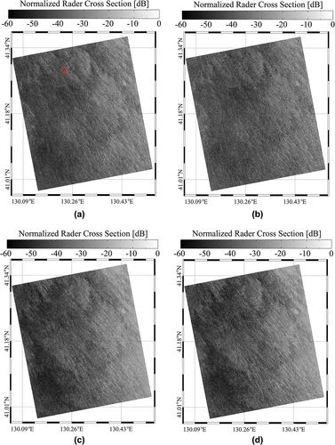
where ${\sigma }_0$ is the NRCS (dB), which is dependent on polarization; DN is the digital number; and M and N are constants annotated with SAR raw data. It is necessary to determine if the historical GF-3 image has been recalibrated since November 2019 to improve the imaging quality of the image. The GF-3 SAR scenes are divided into 256 × 256 pixels sub-scenes with a spatial coverage of 4 km, and the sub-scenes are smoothed using a 3 × 3 Gaussian filter (Zhang et al. 2010b). As examples, the calibrated NRCS maps for 09:13 UTC on 4 April 2020, are shown in Figure 1(a–d), i.e. VV, HH, VH, and HV polarization, respectively.

Figure 1. NRCS maps of GF-3 SAR image acquired at 09:13 UTC on 4 April 2020: (a) vertical–vertical polarization; (b) horizontal–horizontal polarization; (c) vertical–horizontal polarization; and (d) horizontal–vertical polarization.

2.2 Hindcast waves from SWAN

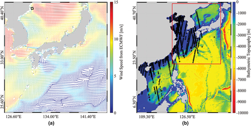
Since there are no available measurements from moored buoys in the coastal China Seas, a third-generation numerical model, i.e. the SWAN model, is employed to simulate the wave fields (Yang et al. 2020), which uses unstructured grids for the complicated shoreline. The European Centre for Medium-Range Weather Forecasts (ECMWF) wind data with 0.5° grids and an interval of 1 h is treated as the forcing field, and the water depth with a 1 km spatial resolution is extracted from the General Bathymetric Chart of the Oceans (GEBCO). The SWAN-simulated wave fields have been used for the validation of the wave retrieval algorithm for GF-3 images (Shao et al. 2022). The outputs include the one-dimensional wave spectrum and the SWH with a 1 km spatial resolution at intervals of 30 min. As an example, the wind map from the ECMWF for 09:00 UTC on 4 April 2020 is shown in Figure 2(a), and the water depth map overlain on all of the collected images, represented by the black rectangles, is presented in Figure 2(b). The time difference between the SAR scene and the ECMWF wind data is less than 15 min.

Figure 2. (a) Wind map from the European Centre for ECMWFfor 09:00 UTC on 4 April 2020. (b) Water depth map extracted from GEBCO. The black rectangle represents the spatial coverage of the image in Figure 1. The red rectangle in Figure (b) represents the area shown in Figure (a).

2.3. Measurements from HY-2B

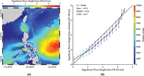
The product of the Chinese HY-2B satellite, which is the successor of the HY-2A satellite launched in 2011, has been operationally released since 2018. The wind vector with 0.25° grids and the SWH following the satellite’s footprint are measured using the HY-2B scatterometer and altimeter, respectively. Both the wind and wave products have a good performance under low-to-moderate wind conditions (Shao et al. 2021), yielding a Root Mean Square Error (RMSE) of 0.78 m/s and a Correlation Coefficient (COR) of 0.97 for the wind speed and a RMSE of 0.29 m and a COR of 0.98 for the SWH comparing with geophysical data record products and the data derived from the advanced scatterometer and Jason-3 altimeter. In this paper, the well-calibrated wind products from the HY-2B scatterometer are used to validate the wind retrievals from GF-3 images. In addition, the SWAN-simulated waves are compared with the products from the HY-2B altimeter to ensure the applicability of the modeling results in the coastal China seas. Figure 3 presents the wind map from the HY-2B scatterometer at 08:00 UTC on 4 April 2020, in which the black rectangle denotes the spatial coverage of the image in Figure 1. The SWAN-simulated wave map overlain by the footprints from the HY-2B altimeter at 10:00 UTC on 23 January 2020 is shown in Figure 4(a), and the statistical analysis of the SWH yields an RMSE of 0.56 m and a COR of 0.87 for all of the images (Figure 4(b)).

Figure 3. Wind map from HY-2B scatterometer at 08:00 UTC on 4 April 2020, in which the black rectangle denotes the spatial coverage of the image in Figure 1.

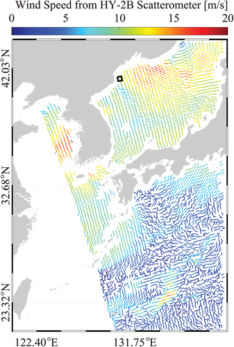
Figure 4. (A) SWAN-simulated wave map overlain by the footprint of the HY-2B altimeter at 10:00 UTC on 23 January 2020. (b) Statistical analysis of the SWH from the SWAN compared with the measurements from HY-2B.

3. Methodology

In this section, the VV-polarized GMF for the SAR wind retrieval is introduced. Then, the fully polarimetric technique for SAR wave retrieval is introduced in detail, in which the improved tilt MTF is used.

3.1. SAR wind retrieval

In the last few decades, scatterometer-based GMFs have been successfully applied for SAR wind retrieval since 1997 due to the similar wind mapping mechanism on the scatterometer and SAR. In principle, a GMF describes a constrained relationship between the intensity of the backscattering signal (i.e. NRCS) and a wind vector. The C-band scatterometer-based GMFs include CMOD4 (Stoffelen and Anderson 1997), CMOD5 (Hersbach, Stoffelen, and Haan 2007), and CMOD7 (Stoffelen et al. 2017). These GMFs restrict work at low-to-moderate winds, although CMOD5N (Hersbach 2010) has a slightly improved performance for wind speeds of up to 33 m/s. Utilizing SAR measurements, the latest CMOD family includes GMF C-SARMOD2 for R-2 and CSARMOD-GF for GF-3. The conventional formulation of the GMF is as follows:

(2) ${\sigma }_0^{pp}(U_{10},\phi ,\theta )=1+B_1(U_{10},\theta )\mathrm{c}\mathrm{o}\mathrm{s}\phi +B_2(U_{10},\theta )\mathrm{c}\mathrm{o}\mathrm{s}2\phi$(2)

where ${\sigma }_0$ is the NRCS (dB); pp is the polarization denoted as VV or HH; U₁₀ is the sea surface wind speed at a height of 10 m; θ is the radar incidence angle; φ is the wind direction relative to the radar look direction; and the coefficients Bs are a function of U₁₀ and θ. It should be noted that the wind speed can also be inverted from a VH-polarized GF-3 SAR image (Zhu et al. 2019a). However, the accuracy relies on the high quality of the noise-equivalent sigma zero, and the wind direction cannot be obtained on VH-polarized SAR. Thus, the wind vector is inverted from the VV-polarized GF-3 image using CSARMOD-GF.

When applying the VV-polarized GMF, the prior information about the wind direction is necessary, because two unknown variables can never be solved using one equation. It is revealed that the pattern on the two-dimensional SAR image spectrum for wavelengths of 800–3000 m is vertical to the true wind direction (Alpers and Brummer, 1994), indicating that the wind direction inverted using the spectrum transformation method has a 180° ambiguity. The swath coverage of the QPS GF-3 SAR is 50 km when the variation in the wind direction is slight. In this case, the 0.25° gridded wind directions from HY-2B are employed to remove this ambiguity. However, the other sea surface dynamics captured by the SAR often distort the wind patterns at the kilometer scale, resulting in difficulty in retrieving the wind directions over the entire image. The technique based on the Cressman interpolation method is used (Shao et al. 2019).

(3) ${\phi }_i={\phi }_0+{\sum }_{k=1}^n\frac{D_k^2-R^2}{D_k^2+R^2}\mathrm{\Delta }{\phi }_k$(3)

In region i, where the spectrum transformation method does not work, φ₀ is the known wind direction of the region nearest to i; R is a constant (set as 5 km); D_k is the distance from region i to k within 5 km; Δφ_k is the difference between the wind direction φ₀ and the referred wind direction φ_k; and φ_i is the interpolated value.

3.2. SAR wave retrieval

For a polarimetric SAR system, the backscattering cross section ${\sigma }_0(\chi ,\varphi )$ at ellipticity $\chi$ and a specific polarization orientation $\varphi$ is determined from the Stokes matrix M and the transmitted and received polarization vectors (Zyl, Zebker, and Elachi 1987):

(4) ${\sigma }_0(\chi ,\varphi )=\frac{4\pi }{{\mathrm{k}}^2}\left[\begin{array}{c}1\\ \mathrm{c}\mathrm{o}\mathrm{s}2\chi \mathrm{c}\mathrm{o}\mathrm{s}2\varphi \\ \mathrm{c}\mathrm{o}\mathrm{s}2\chi \mathrm{s}\mathrm{i}\mathrm{n}2\varphi \\ \mathrm{s}\mathrm{i}\mathrm{n}2\varphi \end{array}\right]\left[\begin{array}{c}{\mathit{M}}_{11}{\mathit{M}}_{12}{\mathit{M}}_{13}{\mathit{M}}_{14}\\ {\mathit{M}}_{21}{\mathit{M}}_{22}{\mathit{M}}_{23}{\mathit{M}}_{24}\\ {\mathit{M}}_{31}{\mathit{M}}_{32}{\mathit{M}}_{33}{\mathit{M}}_{34}\\ {\mathit{M}}_{41}{\mathit{M}}_{42}{\mathit{M}}_{43}{\mathit{M}}_{44}\end{array}\right]\left[\begin{array}{c}1\\ \mathrm{c}\mathrm{o}\mathrm{s}2\chi \mathrm{c}\mathrm{o}\mathrm{s}2\varphi \\ \mathrm{c}\mathrm{o}\mathrm{s}2\chi \mathrm{s}\mathrm{i}\mathrm{n}2\varphi \\ \mathrm{s}\mathrm{i}\mathrm{n}2\varphi \end{array}\right]$(4)

where k is the transmitted wave number, and the superscript T denotes a matrix transpose. According to the polarimetric theory (Schuler and Lee 1995), the ellipticity $\chi$ is set as zero, and the polarization orientation $\varphi$ is equal to 90° for VV-polarization and 0° for HH-polarization. Therefore, the linear backscattering cross section ${\sigma }_0(0,\varphi )$ at polarization orientation $\varphi$ becomes

(5) ${\sigma }_0(\chi ,\varphi )=\frac{4\pi }{k^2}({\mathit{M}}_{11}+{\mathit{M}}_{33}\mathrm{s}\mathrm{i}{\mathrm{n}}^{2}2\varphi +{\mathit{M}}_{11}\mathrm{c}\mathrm{o}{\mathrm{s}}^{2}2\varphi +2{\mathit{M}}_{12}\mathrm{c}\mathrm{o}\mathrm{s}2\varphi )$(5)

in which the Stokes matrix M is proportional to the polarized NRCS. The value of the linear backscattering cross section ${\sigma }_0(0,\varphi )$ is simplified as follows:

(6) $\begin{array}{rl}& {\sigma }_0(0,\varphi )=\frac{1}{4}({\sigma }_0^{\mathrm{h}\mathrm{h}}+{\sigma }_0^{\mathrm{v}\mathrm{v}})(1+\mathrm{c}\mathrm{o}{\mathrm{s}}^{2}2\varphi )+\frac{1}{2}({\sigma }_0^{\mathrm{h}\mathrm{h}}-{\sigma }_0^{\mathrm{v}\mathrm{v}})\mathrm{c}\mathrm{o}\mathrm{s}2\varphi \\ & +{\sigma }_0^{\mathrm{h}\mathrm{v}}+\frac{1}{2}\times \mathrm{\Re }({\sigma }_0^{\mathrm{h}\mathrm{h}\mathrm{v}\mathrm{v}})\times \mathrm{s}\mathrm{i}{\mathrm{n}}^{2}2\varphi \end{array}$(6)

in which ${\sigma }_0^{pp}$ is the SAR-measured NRCS in pp-polarization (i.e. VV, HH, VH, and HV) and $\Re \left[{\sigma }_{\text{0}}^{\text{hhvv}}\right]$ is the real parts of the correlation between ${\sigma }_0^{\mathrm{v}\mathrm{v}}$ and ${\sigma }_0^{\mathrm{h}\mathrm{h}}$. The linearly polarized backscattering cross section at polarization orientation $\varphi$ can be estimated using the above equation and the fully polarized (VV, HH, and HV) NRCS.

According to Bragg resonance theory, the backscattering cross section ${\sigma }_0(r,t)$ in the slant direction $r$ and time dimension t is expressed as

(7) ${\sigma }_0(r,t)={\bar{\sigma }}_0\left\{1+\left[\sum _k{T}^S\xi \left(r,t\right)+c.c^{\ast }\right]\right\}$(7)

where

(8) $T^S=T^{tilt}+T^{hyd}+T^{vb}$(8)

(9) $\xi (r,t)=\sum _k{\xi }_k\mathrm{e}\mathrm{x}\mathrm{p}i\left(kr-\omega t\right)$(9)

In Equations (7–9), ${\bar{\sigma }}_0$ is the spatially averaged specific cross section; ω is the angular wave frequency; c.c * is the complex conjugate of the series; $T^{tilt}$ is the tilt MTF; $T^{hyd}$ is the MTF of the hydrodynamic modulation; and $T^{vb}$ is the MTF caused by nonlinear velocity bunching. Since hydrodynamic modulation and velocity bunching are independent of the polarization, the backscattering cross section modulation between polarization orientation $\varphi$ and co-polarization is expressed as follows:

(10) $\frac{\mathrm{\Delta }{\sigma }_0^{\varphi }}{{\bar{\sigma }}_0^{\varphi }}-\frac{\mathrm{\Delta }{\sigma }_0^{\mathrm{v}\mathrm{v}}}{{\bar{\sigma }}_0^{\mathrm{v}\mathrm{v}}}=\sum _k(T_{\varphi }^{tilt}-T_{\mathrm{v}\mathrm{v}}^{tilt}){\xi }_k\mathrm{e}\mathrm{x}\mathrm{p}i\left(kr-\omega t\right)+R^{\ast }$(10)

(11) $\frac{\mathrm{\Delta }{\sigma }_0^{\varphi }}{{\bar{\sigma }}_0^{\varphi }}-\frac{\mathrm{\Delta }{\sigma }_0^{\mathrm{h}\mathrm{h}}}{{\bar{\sigma }}_0^{\mathrm{h}\mathrm{h}}}=\sum _k(T_{\varphi }^{tilt}-T_{\mathrm{h}\mathrm{h}}^{tilt}){\xi }_k\mathrm{e}\mathrm{x}\mathrm{p}i\left(kr-\omega t\right)+R^{\ast }$(11)

in which R^* is the complex conjugate of the series. By substituting Equation 9(9) $\xi (r,t)=\sum _k{\xi }_k\mathrm{e}\mathrm{x}\mathrm{p}i\left(kr-\omega t\right)$(9) into the above equations, the expressions can be re-written as follows:

(12) $\frac{\mathrm{\Delta }{\sigma }_0^{\varphi }}{{\bar{\sigma }}_0^{\varphi }}-\frac{\mathrm{\Delta }{\sigma }_0^{\mathrm{v}\mathrm{v}}}{{\bar{\sigma }}_0^{\mathrm{v}\mathrm{v}}}=(T_{\varphi }^{tilt}-T_{\mathrm{v}\mathrm{v}}^{tilt})\frac{\mathrm{\partial }\xi }{\mathrm{\partial }\mathrm{r}}$(12)

(13) $\frac{\mathrm{\Delta }{\sigma }_0^{\varphi }}{{\bar{\sigma }}_0^{\varphi }}-\frac{\mathrm{\Delta }{\sigma }_0^{\mathrm{h}\mathrm{h}}}{{\bar{\sigma }}_0^{\mathrm{h}\mathrm{h}}}=(T_{\varphi }^{tilt}-T_{\mathrm{h}\mathrm{h}}^{tilt})\frac{\mathrm{\partial }\xi }{\mathrm{\partial }\mathrm{r}}$(13)

As concluded by Alpers et al. (1986), the tilt MTF can be decomposed into components perpendicular to (k_x) and parallel to (k_l), the radar look direction:

(14) $T_{\varphi }^{tilt}=i{k}_{l}A+ikxB$(14)

The details of $T_{\varphi }^{tilt}$ at polarization orientation $\varphi$ are listed in Appendix A (He et al. 2004). Considering the specific polarization orientation in VV ($\varphi$ = 90°) and HH polarization ($\varphi$ = 0°), the coefficient B is assumed to be zero. Finally, the algebraic expressions can be simplified as follows:

(15) $\frac{\mathrm{\Delta }{\sigma }_0^{\varphi }}{{\bar{\sigma }}_0^{\varphi }}-\frac{\mathrm{\Delta }{\sigma }_0^{\mathrm{v}\mathrm{v}}}{{\bar{\sigma }}_0^{\mathrm{v}\mathrm{v}}}=(T_{k_{l,}\varphi }^{tilt}-T_{k_{l,\mathrm{v}\mathrm{v}}}^{tilt})\frac{\mathrm{\partial }\xi }{\mathrm{\partial }l}+(T_{k_{x,}\varphi }^{tilt}-T_{k_{x,\mathrm{v}\mathrm{v}}}^{tilt})\frac{\mathrm{\partial }\xi }{\mathrm{\partial }x}$(15)

(16) $\frac{\mathrm{\Delta }{\sigma }_0^{\varphi }}{{\bar{\sigma }}_0^{\varphi }}-\frac{\mathrm{\Delta }{\sigma }_0^{\mathrm{h}\mathrm{h}}}{{\bar{\sigma }}_0^{\mathrm{h}\mathrm{h}}}=(T_{k_{l,}\varphi }^{tilt}-T_{k_{l,\mathrm{h}\mathrm{h}}}^{tilt})\frac{\mathrm{\partial }\xi }{\mathrm{\partial }l}+(T_{k_{x,}\varphi }^{tilt}-T_{k_{x,\mathrm{h}\mathrm{h}}}^{tilt})\frac{\mathrm{\partial }\xi }{\mathrm{\partial }x}$(16)

in which $\mathrm{\partial }\xi /\mathrm{\partial }l$ and $\mathrm{\partial }\xi /\mathrm{\partial }x$ are the wave slope spectrum in the range and azimuth directions, respectively. The formulation of the tilt MTF that considers the effect of the wind is presented in Appendix B (Zhang et al. 2021). The root mean square of slope S_rms (see Equation 17(17) $S_{rms}=\sqrt{{\left(\frac{\mathrm{\partial }\xi }{\mathrm{\partial }l}\times \mathrm{s}\mathrm{i}\mathrm{n}\psi \right)}^2+{\left(\frac{\mathrm{\partial }\xi }{\mathrm{\partial }x}\times \mathrm{c}\mathrm{o}\mathrm{s}\psi \right)}^2}$(17) ) is calculated using the wave slope components and the wave-slope direction $\psi$. The SWH H_s is calculated using Equation 18(18) $H_s=2\sqrt{2}\times S_{rms}$(18) (Zhu et al. 2019a):

(17) $S_{rms}=\sqrt{{\left(\frac{\mathrm{\partial }\xi }{\mathrm{\partial }l}\times \mathrm{s}\mathrm{i}\mathrm{n}\psi \right)}^2+{\left(\frac{\mathrm{\partial }\xi }{\mathrm{\partial }x}\times \mathrm{c}\mathrm{o}\mathrm{s}\psi \right)}^2}$(17)

(18) $H_s=2\sqrt{2}\times S_{rms}$(18)

4. Results and discussion

In this section, the winds retrieved from VV-polarized GF-3 images are compared with the measurements from the HY-2B scatterometer, which are used in wave retrieval by applying the fully polarimetric technique. The validation of the inverted SWH retrievals against the HY-2B altimeter is presented. Finally, the variation in the SWH retrievals concerning wave breaking is discussed.

4.1. Validation of wind retrieval

Figure 5 illustrates the SAR intensity spectrum for wavelengths of 800–3000 m, corresponding to the red region in Figure 1, in which the red line represents the wind direction. Then, the low-resolution HY-2B wind direction is applied to remove the 180° ambiguity (Figure 6). The green rectangle in Figure 6 represents the spatial coverage of the GF-3 image. It is determined that the wind directions are not obtained from the inhomogeneous scenes where the ratio between the image variance and the mean squared image is greater than 1.05 (Ding et al. 2019). The wind directions are obtained using the interpolation technique over the entire image, which is required for wind speed retrieval using GMF CSARMOD-GF.

Figure 5. SAR intensity spectrum corresponding to the black region in Figure 1, in which the black line represents the wind direction after removing the 180° ambiguity. The black circular lines represent the wave numbers.

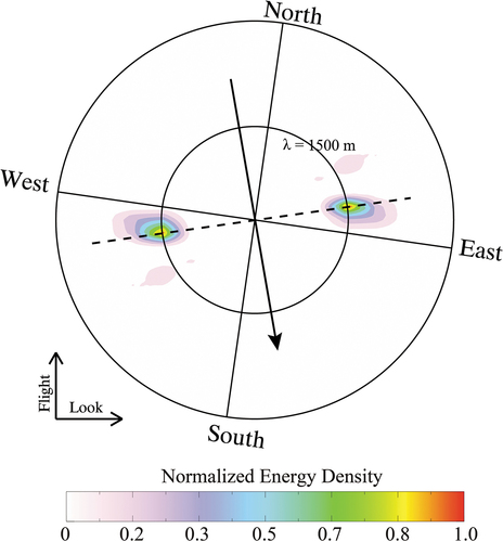
Figure 6. Wind directions from the SAR image corresponding to the image in Figure 1, in which the red vectors represent the HY-2B wind directions.

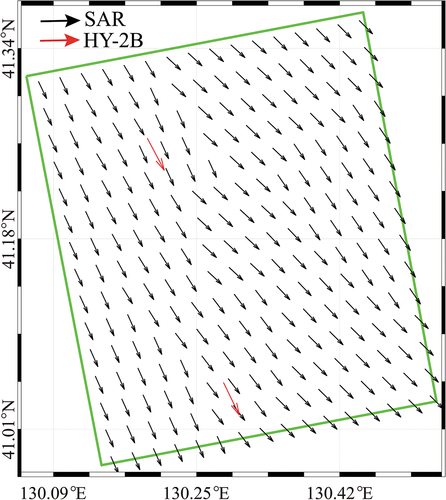
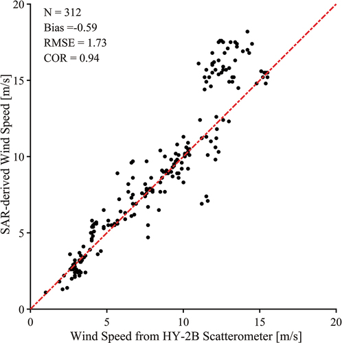
The inverted wind map from the VV-polarized GF-3 image is shown in Figure 7. The sub-scenes of the GF-3 SAR images in 2018–2019 covering the available swath data from the HY-2B scatterometer are used here. In particular, the time difference between them is less than 2 h. A total of approximately 200 matchups are analyzed to assess the accuracy of the SAR-derived wind directions and speeds. Figure 8 presents a comparison using a scatter diagram, yielding an RMSE of 1.73 m/s and a COR of 0.94 for the wind speed. Based on the validation, it is concluded that the inverted winds are reliable for wave retrievals from quad-polarized GF-3 images.

Figure 7. Wind map inverted from the VV-polarized GF-3 image acquired at 09:13 UTC on 4 April 2020, using the GMF CSARMOD-GF.

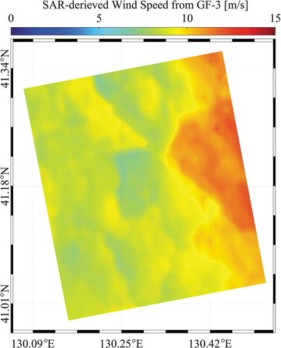
Figure 8. Validation of SAR-derived wind speeds against the available measurements from the HY-2B scatterometer.

4.2. Validation of wave retrieval

The wave retrieval using the full polarimetric technique includes three steps: (1) estimation of the linear backscattering cross section at a polarization orientation of 45° in Equation 6(6) $\begin{array}{rl}& {\sigma }_0(0,\varphi )=\frac{1}{4}({\sigma }_0^{\mathrm{h}\mathrm{h}}+{\sigma }_0^{\mathrm{v}\mathrm{v}})(1+\mathrm{c}\mathrm{o}{\mathrm{s}}^{2}2\varphi )+\frac{1}{2}({\sigma }_0^{\mathrm{h}\mathrm{h}}-{\sigma }_0^{\mathrm{v}\mathrm{v}})\mathrm{c}\mathrm{o}\mathrm{s}2\varphi \\ & +{\sigma }_0^{\mathrm{h}\mathrm{v}}+\frac{1}{2}\times \mathrm{\Re }({\sigma }_0^{\mathrm{h}\mathrm{h}\mathrm{v}\mathrm{v}})\times \mathrm{s}\mathrm{i}{\mathrm{n}}^{2}2\varphi \end{array}$(6) ; (2) inversion of the wave slope using Equation 15(15) $\frac{\mathrm{\Delta }{\sigma }_0^{\varphi }}{{\bar{\sigma }}_0^{\varphi }}-\frac{\mathrm{\Delta }{\sigma }_0^{\mathrm{v}\mathrm{v}}}{{\bar{\sigma }}_0^{\mathrm{v}\mathrm{v}}}=(T_{k_{l,}\varphi }^{tilt}-T_{k_{l,\mathrm{v}\mathrm{v}}}^{tilt})\frac{\mathrm{\partial }\xi }{\mathrm{\partial }l}+(T_{k_{x,}\varphi }^{tilt}-T_{k_{x,\mathrm{v}\mathrm{v}}}^{tilt})\frac{\mathrm{\partial }\xi }{\mathrm{\partial }x}$(15) and Equation 16(16) $\frac{\mathrm{\Delta }{\sigma }_0^{\varphi }}{{\bar{\sigma }}_0^{\varphi }}-\frac{\mathrm{\Delta }{\sigma }_0^{\mathrm{h}\mathrm{h}}}{{\bar{\sigma }}_0^{\mathrm{h}\mathrm{h}}}=(T_{k_{l,}\varphi }^{tilt}-T_{k_{l,\mathrm{h}\mathrm{h}}}^{tilt})\frac{\mathrm{\partial }\xi }{\mathrm{\partial }l}+(T_{k_{x,}\varphi }^{tilt}-T_{k_{x,\mathrm{h}\mathrm{h}}}^{tilt})\frac{\mathrm{\partial }\xi }{\mathrm{\partial }x}$(16) ; and (3) calculation of the SWH H_s using Equation 17(17) $S_{rms}=\sqrt{{\left(\frac{\mathrm{\partial }\xi }{\mathrm{\partial }l}\times \mathrm{s}\mathrm{i}\mathrm{n}\psi \right)}^2+{\left(\frac{\mathrm{\partial }\xi }{\mathrm{\partial }x}\times \mathrm{c}\mathrm{o}\mathrm{s}\psi \right)}^2}$(17) and Equation 18.(18) $H_s=2\sqrt{2}\times S_{rms}$(18) Figure 9 shows the NRCS maps (256 × 256 pixels) extracted from the black region in Figure 1(a–d) present the maps for the VV-polarization channel, HH-polarization channel, HV-polarization channel, and polarization orientation of 45°, respectively. The inverted two-dimensional SAR slope spectrum of the sub-scene in polar coordinates and the one-dimensional wave slope spectrum are presented in Figure 10(a,b), respectively. In this case, the SAR-derived SWH is 1.92 m, and the value simulated using the SWAN model is 2.29 m. For this case, by applying the algorithm for wave retrieval over the entire image in Figure 1, the inverted SWH map overlaid on the simulated waves from the SWAN is displayed in Figure 11.

Figure 9. Sub-scenes extracted from the black region in Figure 1: (a) map for the VV-polarization channel; (b) map for the HH-polarization channel; (c) map for the HV-polarization channel; and (d) map for the polarization orientation of 45°.

Figure 10. (a) Inverted two-dimensional SAR slope spectrum of the sub-scene in polar coordinates and (b) the one-dimensional wave slope spectrum.

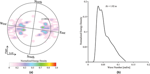
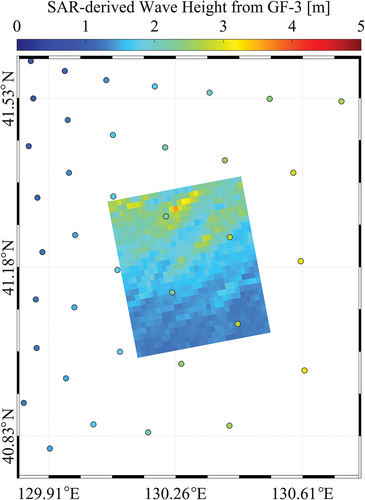
Figure 11. Inverted SWH map from the VV-polarized GF-3 image acquired at 09:13 UTC on 4 April 2020, in which the spots represent the SWAN-simulated results.

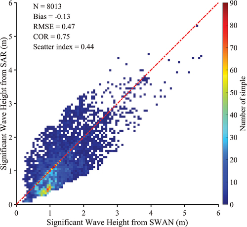
The sub-scenes extracted from the collected GF-3 images are exploited to evaluate the accuracy of the SAR-derived SWHs, which are validated against the available simulations using the SWAN model. A comparison using a scatter diagram of more than 8000 matchups is shown in Figure 12, yielding an RMSE of 0.47 m, a COR of 0.75 and a Scatter Index (SI) of 0.44 for the SWH. It is commonly recognized that the SI of SAR retrieval SWH by empirical models is less than 0.2 (Pleskachevsky et al. 2022). Collectively, although the full polarimetric technique is a promising approach for wave spectrum retrieval from QPS GF-3 images, the accuracy of retrievals necessitates to be further improved.

Figure 12. Comparison of SAR-derived SWHs with the collocated results simulated using the SWAN model.

4.3. Discussion

Wave breaking commonly occurs with wave propagation (De Macedo et al. 2022). The non-polarized (NP) contribution to the NRCS, which is caused by wave breaking, has been recently studied using dual-polarized (VV and HH) GF-3 and TS-X images (Kudryavtsev et al. 2013; Li et al. 2017; Zhong et al. 2023). The fully polarimetric technique takes advantage of the distribution of the NRCS in different polarizations; therefore, the wave breaking supposedly influences the SAR wave retrieval. The NP contribution to the NRCS ${\sigma }_0^{wb}$ is calculated using a theoretical approach that uses the VV-polarized NRCS ${\sigma }_0^{\mathrm{v}\mathrm{v}}$, HH-polarized NRCS ${\sigma }_0^{\mathrm{h}\mathrm{h}}$, SAR-derived wind speed U₁₀, and radar incidence angle θ. The details are presented in Appendix C. 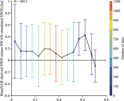Figure 13 shows the variation in the bias (SAR-derived minus SWAN-simulated SWH) with respect to the (${\sigma }_0^{wb}$/${\sigma }_0^{\mathrm{v}\mathrm{v}}$) ratio. It is found that the bias increases as the ratio (>0.4) increases. It is reasonable that the whitecaps produced by wave breaking change the orientation normal to the facet of the long wave, which could reduce the effect of the tilt modulation on the SAR. For ratios less than 0.4, the non-linear effect caused by velocity bunching is significantly reduced, indicating that the linear tilt and hydrodynamic modulation dominate the sea surface. This behavior results in a decrease in the bias at ratios less than 0.4. For ratios greater than 0.6, the linear tilt mainly affects the wave retrieval algorithm. Following this assumption, the wave breaking has to be considered in the wave retrieval using the fully polarimetric technique under extreme sea states, such as typhoons and hurricanes.

Figure 13. Variation in the bias (SAR-derived minus SWAN-simulated SWH) with respect to the ratio of the NRCS in wave breaking to the SAR-measured NRCS (${\sigma }_0^{wb}$/${\sigma }_0^{\mathrm{v}\mathrm{v}}$).

5. Conclusions

Because of the fine spatial resolution and wide swath coverage, SAR is a useful remote-sensing sensor for wind and wave monitoring. The Chinese civilian SAR satellite, called GF-3, was successfully launched in 2016, and the data obtained have been continuously released. Wind retrieval algorithms have been adopted for GF-3, i.e. CSARMOD-GF (Shao et al. 2021), which has been specifically re-tuned for re-calibrated GF-3 and the analytical approach in the nearshore waters of China’s seas (Yao et al. 2022). The improvement of the wave retrieval for co-polarized GF-3 is ongoing in two aspects: a theoretical method based on a mapping mechanism (Zhu et al. 2019b) and an empirical model (Sheng et al. 2018). GF-3 provides two imaging modes operating in quad-polarization, i.e. QPS and wave modes. In this study, we focused on wave retrieval from QPS GF-3 images using a full polarimetric technique. In particular, the empirical tilt MTF, including the effect of the wind speed (Zhang et al. 2021), was used.

More than 1300 quad-polarized GF-3 images were collocated with the wind measurements from HY-2B and wave simulations from SWAN in 2020–2021. The wind directions were obtained from these images in the VV-polarization channel via the spectrum transformation method. Then, the wind speeds were inverted using the VV-polarized GMF CSARMOD-GF, which is applicable for re-calibrated GF-3 images. The validations of the SAR-derived wind speeds and the SWAN-simulated SWH against the measurements from the HY-2B scatterometer and altimeter yielded a RMSE of 1.73 m/s and a COR of 0.94 for the wind speeds, and a RMSE of 0.51 m and a COR of 0.75 for the SWH. The wave slope spectrum was retrieved from quad-polarized images using the VV, HH, and HV-polarized NRCS, and then, the SWH was directly calculated from the inverted wave slope spectrum. The SAR-derived SWHs were compared with the collocated simulations using the SWAN model, yielding a RMSE of 0.47 m, a COR of 0.75, and a 0.44 SI. The accuracy is anticipated to be further improved to be SI less than 0.2. In addition, the dependence of the NP wave breaking on the wave retrieval was studied through the variation in the bias (SAR-derived minus SWAN-simulated SWH) because the NP contribution modulates the sea surface roughness. It was found that the bias significantly increased as the ratio (${\sigma }_0^{wb}$/${\sigma }_0^{\mathrm{v}\mathrm{v}}$) (>0.4) increased, whereas the bias gradually decreased at ratios less than 0.4. It is not surprising that wave breaking influences the tilt modulation because breaking-induced whitecaps change the angle of the radar beam reflected from the sea surface.

Until now, the TC wind field has been conveniently inverted from VH-polarized SAR images in the C-band, e.g. the R-2 (Zhang et al. 2010b), S-1 (Gao et al. 2020), and GF-3 (Shao et al. 2018). In the future, the tilt MTF in VH-polarization should be studied using SAR images acquired during TCs. Then, it is anticipated that the TC waves can be inverted using the polarimetric technique. In particular, the wave breaking should be considered in the retrieval scheme.

Acknowledgements

We are truly thankful to the National Ocean Satellite Application Center (NSOAS) for providing the Gaofen-3 (GF-3) SAR images and the products from Haiyang-2B (HY-2B) (https://osdds.nsoas.org.cn). The original code of the simulating waves nearshore model was officially released by the Delft University of Technology. The European Centre for Medium-Range Weather Forecasts data were downloaded from http://www.ecmwf.int, and the General Bathymetric Chart of the Oceans data were obtained from ftp.edcftp.cr.usgs.gov.

Disclosure statement

No potential conflict of interest was reported by the author(s).

Data availability statement

Due to the nature of this research, the participants of this study did not agree for their data to be shared publicly, so the supporting data are not available.

Additional information

Funding

This research was partially supported by the National Natural Science Foundation of China [grant number 42076238] and the Natural Science Foundation of Shanghai [grant number 23ZR1426900].

Notes on contributors

Weizeng Shao

Weizeng Shao received his PhD from the Ocean University of China and is currently a full professor of physical oceanography at Shanghai Ocean University. His research interests include numerical simulation of ocean waves, typhoon process, ocean waves, and small-scale air–sea interactions. Currently, he has published more than 50 peer-reviewed papers in the field of SAR oceanography and ocean wave modeling.

Yuyi Hu

Yuyi Hu is currently pursuing a PhD at Shanghai Ocean University. His research interests include the investigation of ocean waves using the remote sensing and numerical modeling techniques.

Xingwei Jiang

Xingwei Jiang received her PhD in science and became an academician at the Chinese Academy of Engineering and a doctoral supervisor. She is currently the Director of the Chinese National Satellite Marine Application Center and the chief designer of the Chinese marine satellite ground application system. She was the Vice Chairman of the Chinese Ocean Society and the China Association for Remote Sensing Applications. She was the Chairman of the Ocean Remote Sensing Professional Committee of the Chinese Ocean Society and was a member of the International GEO Organization Technical Coordination Group and the Sino-French Marine Satellite Joint Steering Committee.

Youguang Zhang

Youguang Zhang received his PhD in Ocean Remote Sensing from the Institute of Oceanology, Chinese Academy of Sciences, China, in 2004. His research has focused on the processing and application of satellite altimeter and satellite wave spectrometer data, and technology for calibrating marine microwave remote sensors. He was the Deputy Chief of the HY-2 Satellite Ground System and the Ocean Salinity Satellite Ground System. He was a member of the construction of the marine satellite ground application system project, the Chinese manned space project Shenzhou 4 multi-modal microwave remote sensor data processing, the HY-2 satellite pre-research project, (He) the Chinese civil aerospace special scientific research pre-research, the Chinese 863 marine remote sensing calibration and inspection technology and the Chinese national defense pre-research and provincial and ministerial fund projects.

Appendices Appendix A

As explicitly illustrated by He et al. (2004), the component of the tilt MTF at polarization orientation ϕ in the radar look direction k_l and radar flight direction k_x is stated as follows:

(A1) $T_{k_{l,}\varphi }^{tilt}=\frac{i{k}_l}{A_0}\left[4\mathrm{c}\mathrm{o}{\mathrm{s}}^{-2}\theta \mathrm{s}\mathrm{i}{\mathrm{n}}^{-1}2\theta \left(1+co{\mathrm{s}}^{2}2\varphi \right)-8\mathrm{t}\mathrm{a}{\mathrm{n}}^2\theta \mathrm{s}\mathrm{i}{\mathrm{n}}^{-1}2\theta \mathrm{c}\mathrm{o}\mathrm{s}2\varphi +2{\left(\mathrm{c}\mathrm{o}{\mathrm{s}}^3\theta \mathrm{s}\mathrm{i}\mathrm{n}\theta \right)}^{-1}\mathrm{s}\mathrm{i}{\mathrm{n}}^{2}2\varphi \right]$(A1)

(A2) $T_{k_{x,}\varphi }^{tilt}=-\frac{i{k}_x}{A_0}\left[\left(1+(\frac{1+si{\mathrm{n}}^2\theta }{\mathrm{c}\mathrm{o}{\mathrm{s}}^2\theta }{)}^2\right)\mathrm{c}\mathrm{o}\mathrm{s}2\varphi +\left(1-{(\frac{1+si{\mathrm{n}}^2\theta }{\mathrm{c}\mathrm{o}{\mathrm{s}}^2\theta })}^2\right)-2\left(\frac{1+{\mathrm{s}\mathrm{i}\mathrm{n}}^2\theta }{\mathrm{c}\mathrm{o}{\mathrm{s}}^2\theta }\right)\mathrm{c}\mathrm{o}\mathrm{s}2\varphi \right]\frac{\mathrm{s}\mathrm{i}\mathrm{n}2\varphi }{\mathrm{s}\mathrm{i}\mathrm{n}\theta }$(A2)

where

(A3) $A_0=\frac{1}{4}\left[1+(\frac{1+si{\mathrm{n}}^2\theta }{\mathrm{c}\mathrm{o}{\mathrm{s}}^2\theta }{)}^2\right]\left(1+{\mathrm{c}\mathrm{o}\mathrm{s}}^{2}2\varphi \right)-2\frac{1+\mathrm{s}\mathrm{i}{\mathrm{n}}^2\theta }{\mathrm{c}\mathrm{o}\mathrm{s}4\theta }\mathrm{c}\mathrm{o}\mathrm{s}2\varphi +\frac{1}{2}\left(1+{\mathrm{t}\mathrm{a}\mathrm{n}}^2\theta \right)\mathrm{s}\mathrm{i}{\mathrm{n}}^{2}2\varphi$(A3)

in which i = $\sqrt{-1}$.

Appendix B

The details of the co-polarized (vertical–vertical (VV) and horizontal–horizontal (HH)) Modulation Transfer Functions (MTFs) have the following formulation (Zhang et al. 2021):

(B1) $T_{k_{l,pp}}^{tilt}=i{k}_l\left[a_1{U}_{10}^2+a_2{\phi }^2+a_3{\theta }^2+a_4{U}_{10}\phi +a_5{U}_{10}\theta +a_6\theta \phi +a_7{U}_{10}+a_8\phi +a_9\theta +a_{10}\right]$(B1)

in which$T_{pp}^{tilt}$ is the MTFs in pp-polarization, U₁₀ is the sea surface wind speed at a height of 10 m, θ is the incidence angle, φ is the wind direction, k_l is the wave number in the radar look direction, and the values of coefficients (a) are given in Table A1.

Table A1. Values of coefficients for VV and HH polarization.

	VV polarization	HH polarization
a1	0.007799	0.008398
a2	1.21723e–15	1.226019e–05
a3	0.002941	0.005492
a4	−3.635699e–14	5.00855e–15
a5	0.008508	0.008506
a6	−3.365627e–14	8.150555e–15
a7	−0.685241	−0.714355
a8	1.303660e–12	−3.285571e–13
a9	−0.595169	−0.792862
a10	29.084355	30.901273

Appendix C

The Normalized Radar Cross Section (NRCS) for wave breaking ${\sigma }_0^{wb}$ can be practically calculated using the SAR-measured NRCS in the VV ${\sigma }_0^{\mathrm{v}\mathrm{v}}$and HH ${\sigma }_0^{\mathrm{h}\mathrm{h}}$ polarization channels (Sun et al. 2022):

(C1) ${\sigma }_0^{wb}={\sigma }_0^{\mathrm{v}\mathrm{v}}-\frac{{\sigma }_0^{\mathrm{v}\mathrm{v}}-{\sigma }_0^{\mathrm{h}\mathrm{h}}}{1-p_B}$(C1)

where

(C2) $p_B=\frac{{\left|G_{\mathrm{h}\mathrm{h}}\right|}^2}{{\left|G_{\mathrm{v}\mathrm{v}}\right|}^2}\times \frac{1+g_{\mathrm{h}\mathrm{h}}{s}_i^2}{1+g_{\mathrm{v}\mathrm{v}}{s}_i^2}$(C2)

(C3) ${\left|G_{\mathrm{v}\mathrm{v}}\right|}^2=\frac{\mathrm{c}\mathrm{o}{\mathrm{s}}^2\theta (1+\mathrm{s}\mathrm{i}{\mathrm{n}}^2\theta )}{{(\mathrm{c}\mathrm{o}\mathrm{s}\theta +0.111)}^4}$(C3)

(C4) ${\left|G_{\mathrm{h}\mathrm{h}}\right|}^2=\frac{\mathrm{c}\mathrm{o}{\mathrm{s}}^4\theta }{{(0.111\mathrm{c}\mathrm{o}\mathrm{s}\theta +1)}^4}$(C4)

(C5) $g_{\mathrm{v}\mathrm{v}}=\frac{\mathrm{t}\mathrm{a}{\mathrm{n}}^4\theta }{2{\left|G_{\mathrm{v}\mathrm{v}}\right|}^2}\frac{{\mathrm{\partial }}^2}{\mathrm{\partial }{\theta }^2}(\frac{{\left|G_{\mathrm{v}\mathrm{v}}\right|}^2}{\mathrm{t}\mathrm{a}{\mathrm{n}}^4\theta })$(C5)

(C6) $g_{\mathrm{h}\mathrm{h}}=\frac{\mathrm{t}\mathrm{a}{\mathrm{n}}^4\theta }{2{\left|G_{\mathrm{h}\mathrm{h}}\right|}^2}\frac{{\mathrm{\partial }}^2}{\mathrm{\partial }{\theta }^2}(\frac{{\left|G_{\mathrm{h}\mathrm{h}}\right|}^2}{\mathrm{t}\mathrm{a}{\mathrm{n}}^4\theta })+\frac{2}{\mathrm{s}\mathrm{i}{\mathrm{n}}^2\theta }\frac{\left|G_{\mathrm{h}\mathrm{h}}\right|}{\left|G_{\mathrm{h}\mathrm{h}}\right|}$(C6)

in which θ is the incidence angle. Assuming that the sea surface is tilt modulated by a small mean square slope, the slope s_i can be empirically derived from the wind speed U₁₀ and wave age $\beta$:

(C7) ${s_i}^2=0.00225\times ln(\frac{2kr{U}_{10}^2\mathrm{s}\mathrm{i}\mathrm{n}\theta }{4g{\beta }^2})$(C7)

in which g is the gravitational acceleration, and k_r is the wave number of the radar beam. According to the formulation of the well-known Pierson–Moskowitz wave spectrum, the wave age $\beta$ is directly related to the wind speed U₁₀:

(C8) $\beta =\frac{U_{10}^2}{g}$(C8)

References

- Alpers, W., and B. Brummer. 1994. “Atmospheric Boundary Layer Rolls Observed by the Synthetic Aperture Radar Aboard the ERS-1 Satellite.” Journal of Geophysical Research 99 (C6): 12613–12621. https://doi.org/10.1029/94JC00421.
- Alpers, W., and C. Bruning. 1986. “On the Relative Importance of Motion-Related Contributions to SAR Imaging Mechanism of Ocean Surface Waves.” IEEE Transactions on Geoscience and Remote Sensing 24 (6): 873–885. https://doi.org/10.1109/TGRS.1986.289702.
- Alpers, W., and C. Bruning. 1986. “On the Relative Importance of Motion-Related Contributions to SAR Imaging Mechanism of Ocean Surface Waves.” IEEE Transactions on Geoscience & Remote Sensing 24 (6): 873–885. https://doi.org/10.1109/TGRS.1986.289702.
- Bao, L. W., X. Zhang, C. H. Cao, X. C. Wang, Y. J. Jia, G. Gao, Y. Zhang, Y. Wang, and J. Zhang. 2022. “Impact of Polarization Basis on Wind and Wave Parameters Estimation Using the Azimuth Cutoff from GF-3 SAR Imagery.” IEEE Transactions on Geoscience & Remote Sensing 60:1–16. https://doi.org/10.1109/TGRS.2022.3204409.
- Corcione, V., G. Grieco, M. Portabella, F. Nunzuata, and M. Migliaccio. 2019. “A Novel Azimuth Cutoff Implementation to Retrieve Sea Surface Wind Speed from SAR Imagery.” IEEE Transactions on Geoscience and Remote Sensing 57 (6): 3331–3340. https://doi.org/10.1109/TGRS.2018.2883364.
- De Macedo, C. R., J. C. B. Da Silva, A. Buono, and M. Migliaccio. 2022. “Multi-Polarization Radar Backscatter Signatures of Internal Waves at L-Band.” International Journal of Remote Sensing 43 (6): 1943–1959. https://doi.org/10.1080/01431161.2022.2050435.
- Ding, Y. Y., J. C. Zuo, W. Z. Shao, J. Shi, X. Z. Yuan, J. Sun, J. C. Hu, and X. F. Li. 2019. “Wave Parameters Retrieval for Dual-Polarization C-Band Synthetic Aperture Radar Using a Theoretical-Based Algorithm Under Cyclonic Conditions.” Acta Oceanologica Sinica 38 (5): 21–31. https://doi.org/10.1007/s13131-019-1438-y.
- Fan, C. Q., T. R. Song, Q. S. Yan, J. M. Meng, Y. Q. Wu, and J. Zhang. 2022. “Evaluation of Multi-Incidence Angle Polarimetric Gaofen-3 SAR Wave Mode Data for Significant Wave Height Retrieval.” Remote Sensing 14 (21): 5480. https://doi.org/10.3390/rs14215480.
- Gao, Y., C. L. Guan, J. Sun, and L. A. Xie. 2020. “Tropical Cyclone Wind Speed Retrieval from Dual-Polarization Sentinel-1 EW Mode Products.” Journal of Atmospheric and Oceanic Technology 37 (9): 1713–1724. https://doi.org/10.1175/JTECH-D-19-0148.1.
- Hasselmann, K., and S. Hasselmann. 1991. “On the Nonlinear Mapping of an Ocean Wave Spectrum into a Synthetic Aperture Radar Image spectrum.”Journal of Geophysical Research.” 96 (C6): 10713–10729. https://doi.org/10.1029/91JC00302.
- He, Y. J., W. Perrie, T. Xie, and Q. Zhou. 2004. “Ocean Wave Spectra from a Linear Polarimetric SAR.” IEEE Transactions on Geoscience & Remote Sensing 42 (11): 2623–2631. https://doi.org/10.1109/TGRS.2004.836813.
- Hersbach, H. 2010. “Comparison of C-Band Scatterometer CMOD5.N Equivalent Neutral Winds with ECMWF.” Journal of Atmospheric and Oceanic Technology 27 (4): 721–736. https://doi.org/10.1175/2009JTECHO698.1.
- Hersbach, H., A. Stoffelen, and S. D. Haan. 2007. “An Improved C-Band Scatterometer Ocean Geophysical Model Function: CMOD5.” Journal of Geophysical Research 112 (C3): 3006–3024. https://doi.org/10.1029/2006JC003743.
- He, Y. J., H. Shen, and W. Perrie. 2006. “Remote Sensing of Ocean Waves by Polarimetric SAR.” Journal of Atmospheric and Oceanic Technology 23 (3): 1768–1773. https://doi.org/10.1175/JTECH1948.1.
- Isaksen, L., and A. Stoffelen. 2000. “ERS Scatterometer Wind Data Impact on Ecmwf’s Tropical Cyclone Forecasts.” IEEE Transactions on Geoscience and Remote Sensing 38 (4): 1885–1892. https://doi.org/10.1109/36.851771.
- Jiang, T., W. Z. Shao, Y. Y. Hu, G. Zheng, and W. Shen. 2023. “L-Band Analysis of the Effects of Oil Slicks on Sea Wave Characteristics.” Journal of Ocean University of China 22 (1): 9–20. https://doi.org/10.1007/s11802-023-5172-x.
- Kudryavtsev, V. N., B. Chapron, A. V. Myasoedov, F. Collard, and J. A. Johannessen. 2013. “On Dual Co-Polarized SAR Measurements of the Ocean Surface.” IEEE Transactions on Geoscience and Remote Sensing Letters 10 (4): 761–765. https://doi.org/10.1109/LGRS.2012.2222341.
- Lin, B., W. Z. Shao, X. F. Li, H. Li, X. Q. Du, Q. Y. Ji, and L. N. Cai. 2017. “Development and Validation of an Ocean Wave Retrieval Algorithm for VV-Polarization Sentinel-1 SAR Data.” Acta Oceanologica Sinica 36 (7): 95–101. https://doi.org/10.1007/s13131-017-1089-9.
- Li, J. X., M. Zhang, W. N. Fan, and D. Nie. 2017. “Facet-Based Investigation on Microwave Backscattering from Sea Surface with Breaking Waves: Sea Spikes and SAR Imaging.” IEEE Transactions on Geoscience & Remote Sensing 55 (4): 2313–2325. https://doi.org/10.1109/TGRS.2016.2641682.
- Lu, Y., B. Zhang, W. Perrie, X. F. Li, and H. Wang. 2018. “A C-Band Geophysical Model Function for Determining Coastal Wind Speed Using Synthetic Aperture Radar.” IEEE Journal of Selected Topics in Applied Earth Observations and Remote Sensing 11:2417–2428. https://doi.org/10.1109/JSTARS.2018.2836661.
- Lyzenga, D. R. 1986. “Numerical Simulation of Synthetic Aperture Radar Image Spectra for Ocean Waves.” IEEE Transactions on Geoscience and Remote Sensing 24 (6): 863–872. https://doi.org/10.1109/TGRS.1986.289701.
- Masuko, H., K. Okamoto, M. Shimada, and S. Niwa. 1986. “Measurement of Microwave Backscattering Signatures of the Ocean Surface Using X Band and Ka Band Airborne Scatterometers.” Journal of Geophysical Research 91 (C11): 13065–13083. https://doi.org/10.1029/JC091iC11p13065.
- Monaldo, F. M., C. Jackson, X. F. Li, and W. Pichel. 2016. “Preliminary Evaluation of Sentinel-1A Wind Speed Retrievals.” IEEE Journal of Selected Topics in Applied Earth Observations and Remote Sensing 9 (6): 2638–2642. https://doi.org/10.1109/JSTARS.2015.2504324.
- Mouche, A. A., and B. Chapron. 2016. “Global C-Band Envisat, RADARSAT-2 and Sentinel-1 SAR Measurements in Copolarization and Cross-Polarization.” Journal of Geophysical Research 120 (11): 7195–7207. https://doi.org/10.1002/2015JC011149.
- Pleskachevsky, A., S. Jacobsen, B. Tings, and E. Schwarz. 2019. “Estimation of Sea State from Sentinel-1 Synthetic Aperture Radar Imagery for Maritime Situation Awareness.” International Journal of Remote Sensing 40 (11): 4104–4142. https://doi.org/10.1080/01431161.2018.1558377.
- Pleskachevsky, A. L., W. Rosenthal, and S. Lehner. 2016. “Meteo-Marine Parameters for Highly Variable Environment in Coastal Regions from Satellite Radar Images.” ISPRS Journal of Photogrammetry & Remote Sensing 119:464–484. https://doi.org/10.1016/j.isprsjprs.2016.02.001.
- Pleskachevsky, A., B. Tings, S. Wiehle, J. Imber, and S. Jacobsen. 2022. “Multiparametric Sea State Fields from Synthetic Aperture Radar for Maritime Situational Awareness.” Remote Sensing of Environment 280:113200. https://doi.org/10.1016/j.rse.2022.113200.
- Quach, B., Y. Glaser, J. E. Stopa, A. A. Mouche, and P. Sadowski. 2021. “Deep Learning for Predicting Significant Wave Height from Synthetic Aperture Radar.” IEEE Transactions on Geoscience and Remote Sensing 59 (3): 1859–1867. https://doi.org/10.1109/TGRS.2020.3003839.
- Quilfen, Y., B. Chapron, T. Elfouhaily, K. Katsaros, and J. Tournadre. 1998. “Observation of Tropical Cyclones by High-Resolution Scatterometry.” Journal of Geophysical Research 103 (C4): 7767–7786. https://doi.org/10.1029/97JC01911.
- Schuler, D. L., and J. S. Lee. 1995. “A Microwave Technique to Improve the Measurement of Directional Ocean Wave Spectra.” International Journal of Remote Sensing 16 (2): 199–215. https://doi.org/10.1080/01431169508954390.
- Schulz-Stellenfleth, J., T. Konig, and S. Lehner. 2007. “An Empirical Approach for the Retrieval of Integral Ocean Wave Parameters from Synthetic Aperture Radar Data.” Journal of Geophysical Research 112 (C3): C03019. https://doi.org/10.1029/2006JC003970.
- Schulz-Stellenfleth, J., S. Lehner, and D. Hoja. 2005. “A Parametric Scheme for the Retrieval of Two-Dimensional Ocean Wave Spectra from Synthetic Aperture Radar Look Cross Spectra.” Journal of Geophysical Research 110 (C5): C05004. https://doi.org/10.1029/2004JC002822.
- Shao, W. Z., Y. Y. Hu, F. Nunziata, V. Corcione, and X. M. Li. 2020. “Cyclone Wind Retrieval Based on X-Band SAR-Derived Wave Parameter Estimation.” Journal of Atmospheric and Oceanic Technology 37 (10): 1907–1924. https://doi.org/10.1175/JTECH-D-20-0014.1.
- Shao, W. Z., T. Jiang, X. W. Jiang, Y. G. Zhang, and W. Zhou. 2021. “Evaluation of Sea Surface Winds and Waves Retrieved from the Chinese HY-2B Data.” IEEE Journal of Selected Topics in Applied Earth Observations & Remote Sensing 14 (10): 9624–9635. https://doi.org/10.1109/JSTARS.2021.3112760.
- Shao, W. Z., X. W. Jiang, Z. F. Sun, Y. Y. Hu, A. Marino, and Y. G. Zhang. 2022. “Evaluation of Wave Retrieval for Chinese Gaofen-3 Synthetic Aperture Radar.” Geo-Spatial Information Science 25 (2): 229–243. https://doi.org/10.1080/10095020.2021.2012531.
- Shao, W. Z., Z. Z. Lai, F. Nunziata, A. Buono, X. W. Jiang, and J. C. Zuo. 2022. “Wind Field Retrieval with Rain Correction from Dual-Polarized Sentinel-1 SAR Imagery Collected During Tropical Cyclones.” Remote Sensing 14 (19): 5006. https://doi.org/10.3390/rs14195006.
- Shao, W. Z., F. Nunziata, Y. G. Zhang, V. Corcione, and M. Migliaccio. 2021. “Wind Speed Retrieval from the Gaofen-3 Synthetic Aperture Radar for VV- and HH-Polarization Using a Re-Tuned Algorithm.” European Journal of Remote Sensing 54 (1): 1318–1337. https://doi.org/10.1080/22797254.2021.1924082.
- Shao, W. Z., Y. X. Sheng, and J. Sun. 2017. “Preliminary Assessment of Wind and Wave Retrieval from Chinese Gaofen-3 SAR Imagery.” Sensors 17 (8): 1705. https://doi.org/10.3390/s17081705.
- Shao, W. Z., J. Sun, C. L. Guan, and Z. F. Sun. 2014. “A Method for Sea Surface Wind Field Retrieval from SAR Image Mode Data.” Journal of Ocean University of China 13 (2): 198–204. https://doi.org/10.1007/s11802-014-1999-5.
- Shao, W. Z., X. Z. Yuan, Y. X. Sheng, J. Sun, W. Zhou, and Q. J. Zhang. 2018. “Development of Wind Speed Retrieval from Cross-Polarization Chinese Gaofen-3 Synthetic Aperture Radar in Typhoons.” Sensors 18 (2): 412. https://doi.org/10.3390/s18020412.
- Shao, W. Z., C. Zhao, X. W. Jiang, W. L. Wang, W. Shen, and J. C. Zuo. 2022. “Preliminary Analysis of Wave Retrieval from Chinese Gaofen-3 SAR Imagery in the Arctic Ocean.” European Journal of Remote Sensing 55 (1): 440–452. https://doi.org/10.1080/22797254.2022.2098830.
- Shao, W. Z., S. Zhu, J. Sun, X. Z. Yuan, Y. X. Sheng, Q. J. Zhang, and Q. Y. Ji. 2019. “Evaluation of Wind Retrieval from Co-Polarization Gaofen-3 SAR Imagery Around China Seas.” Journal of Ocean University of China 18 (1): 80–92. https://doi.org/10.1007/s11802-019-3779-8.
- Sheng, Y. X., W. Z. Shao, S. Q. Li, Y. M. Zhang, H. W. Yang, and J. C. Zuo. 2019. “Evaluation of Typhoon Waves Simulated by WaveWatch-III Model in Shallow Waters Around Zhoushan Islands.” Journal of Ocean University of China 18 (2): 365–375. https://doi.org/10.1007/s11802-019-3829-2.
- Sheng, Y. X., W. Z. Shao, S. Zhu, J. Sun, X. Z. Yuan, S. Q. Li, J. Shi, and J. C. Zuo. 2018. “Validation of Significant Wave Height Retrieval from Co-Polarization Chinese Gaofen-3 SAR Imagery.” Acta Oceanologica Sinica 37 (6): 1–10. https://doi.org/10.1007/s13131-018-1217-1.
- Steele, K., J. Lau, and Y. H. Hsu. 1985. “Theory and Application of Calibration Techniques for an NDBC Directional Wave Measurements Buoy.” IEEE Journal of Oceanic Engineering 10 (4): 382–396. https://doi.org/10.1109/JOE.1985.1145116.
- Stoffelen, A., and D. Anderson. 1997. “Scatterometer Data Interpretation: Estimation and Validation of the Transfer Function CMOD4.” Journal of Geophysical Research 102 (C3): 5767–5780. https://doi.org/10.1029/96JC02860.
- Stoffelen, A., J. Verspeek, J. Vogelzang, and A. Verhoef. 2017. “The CMOD7 Geophysical Model Function for ASCAT and ERS Wind Retrievals.” IEEE Journal of Selected Topics in Applied Earth Observations & Remote Sensing 10 (5): 2123–2134. https://doi.org/10.1109/JSTARS.2017.2681806.
- Sun, Y., W. Perrie, and B. Toulany. 2018. “Simulation of Wave-Current Interactions Under Hurricane Conditions Using an Unstructured Grid Model: Impacts on Ocean Waves.” Journal of Geophysical Research 123 (5): 3739–3760. https://doi.org/10.1029/2017JC012939.
- Sun, Z. F., W. Z. Shao, X. W. Jiang, F. Nunziata, W. L. Wang, W. Shen, and M. Migliaccio. 2022. “Contribution of Breaking Wave on the Co-Polarized Backscattering Measured by the Chinese Gaofen-3 SAR.” International Journal of Remote Sensing 43 (4): 1384–1408. https://doi.org/10.1080/01431161.2021.2009150.
- Tolman, H. L., and N. Booij. 1998. “Modeling Wind Waves Using Wave Number Direction Spectra and a Variable Wavenumber Grid.” Global Atmosphere and Ocean System 6 (4): 295–309.
- Wang, H., J. S. Yang, M. S. Lin, W. W. Li, J. H. Zhu, L. Ren, and L. M. Cui. 2022. “Quad-Polarimetric SAR Sea State Retrieval Algorithm from Chinese Gaofen-3 Wave Mode Imagettes via Deep Learning.” Remote Sensing of Environment 273:112969. https://doi.org/10.1016/j.rse.2022.112969.
- Xu, Q., Y. Li, X. F. Li, Z. Zhang, Y. Cao, and Y. C. Cheng. 2018. “Impact of Ships and Ocean Fronts on Coastal Sea Surface Wind Measurements from the Advanced Scatterometer.” IEEE Journal of Selected Topics in Applied Earth Observations & Remote Sensing 11 (7): 2162–2169. https://doi.org/10.1109/JSTARS.2018.2817568.
- Yang, Z. H., W. Z. Shao, Y. Ding, J. Shi, and Q. Y. Ji. 2020. “Wave Simulation by the SWAN Model and FVCOM Considering the Sea-Water Level Around the Zhoushan Islands.” Journal of Marine Science and Engineering 8 (10): 783. https://doi.org/10.3390/jmse8100783.
- Yao, R., W. Z. Shao, X. W. Jiang, and T. Yu. 2022. “Wind Speed Retrieval from Chinese Gaofen-3 Synthetic Aperture Radar Using an Analytical Approach in the Nearshore Waters of China’s Seas.” International Journal of Remote Sensing 43 (8): 3028–3048. https://doi.org/10.1080/01431161.2022.2079019.
- Zecchetto, S., and F. De Biasio. 2008. “A Wavelet-Based Technique for Sea Wind Extraction from SAR Images.” IEEE Transactions on Geoscience & Remote Sensing 46 (10): 2983–2989. https://doi.org/10.1109/TGRS.2008.920967.
- Zhang, B., and W. Perrie. 2012. “Cross-Polarized Synthetic Aperture Radar: A New Potential Technique for Hurricanes.” Bulletin of the American Meteorological Society 93 (4): 531–541. https://doi.org/10.1175/BAMS-D-11-00001.1.
- Zhang, B., W. Perrie, and Y. J. He. 2010a. “Cross-Polarized Synthetic Aperture Radar: A New Potential Technique for Hurricanes.” Bulletin of the American Meteorological Society 93 (4): 531–541. https://doi.org/10.1175/BAMS-D-11-00001.1.
- Zhang, B., W. Perrie, and Y. J. He. 2010b. “Validation of RADARSAT-2 Fully Polarimetric SAR Measurements of Ocean Surface Waves.” Journal of Geophysical Research 115 (C6): C06031. https://doi.org/10.1029/2009JC005887.
- Zhang, Z. X., Y. Q. Qi, P. Shi, C. W. Li, and Y. Li. 2003. “Preliminary Study on Assimilation of Significant Wave Heights from T/P Altimeter.” Acta Oceanologica Sinica 25 (5): 21–28.
- Zhang, Y. M., Y. H. Wang, J. Zhang, and Y. Z. Liu. 2021. “Reanalysis of the Tilt MTFs Based on the C-Band Empirical Geophysical Model Function.” IEEE Geoscience and Remote Sensing Letters 18 (9): 1500–1504. https://doi.org/10.1109/LGRS.2020.3004332.
- Zhong, R. Z., W. Z. Shao, C. Zhao, X. W. Jiang, and J. C. Zuo. 2023. “Analysis of Wave Breaking on Gaofen-3 and TerraSAR-X SAR Image and Its Effect on Wave Retrieval.” Remote Sensing 15 (3): 574. https://doi.org/10.3390/rs15030574.
- Zhu, S., W. Z. Shao, M. Armando, J. Shi, J. Sun, X. Z. Yuan, J. C. Hu, D. K. Yang, and J. C. Zuo. 2019a. “Evaluation of Chinese Quad-Polarization Gaofen-3 SAR Wave Mode Data for Significant Wave Height Retrieval.” Canadian Journal of Remote Sensing 44 (6): 588–600. https://doi.org/10.1080/07038992.2019.1573136.
- Zhu, S., W. Z. Shao, A. Marino, J. Sun, and X. Z. Yuan. 2019b. “Semi-Empirical Algorithm for Wind Speed Retrieval from Gaofen-3 Quad-Polarization Strip Mode SAR Data.” Journal of Ocean University of China 19 (1): 23–35. https://doi.org/10.1007/s11802-020-4215-9.
- Zyl, J., H. A. Zebker, and C. Elachi. 1987. “Imaging Radar Polarization Signatures: Theory and Observation.” Radio Science 22 (4): 529–543. https://doi.org/10.1029/RS022i004p00529.