Integrating vegetation phenological characteristics and polarization features with object-oriented techniques for grassland type identification

ABSTRACT

Due to the small size, variety, and high degree of mixing of herbaceous vegetation, remote sensing-based identification of grassland types primarily focuses on extracting major grassland categories, lacking detailed depiction. This limitation significantly hampers the development of effective evaluation and fine supervision for the rational utilization of grassland resources. To address this issue, this study concentrates on the representative grassland of Zhenglan Banner in Inner Mongolia as the study area. It integrates the strengths of Sentinel-1 and Sentinel-2 active-passive synergistic observations and introduces innovative object-oriented techniques for grassland type classification, thereby enhancing the accuracy and refinement of grassland classification. The results demonstrate the following: (1) To meet the supervision requirements of grassland resources, we propose a grassland type classification system based on remote sensing and the vegetation-habitat classification method, specifically applicable to natural grasslands in northern China. (2) By utilizing the high-spatial-resolution Normalized Difference Vegetation Index (NDVI) synthesized through the Spatial and Temporal Non-Local Filter-based Fusion Model (STNLFFM), we are able to capture the NDVI time profiles of grassland types, accurately extract vegetation phenological information within the year, and further enhance the temporal resolution. (3) The integration of multi-seasonal spectral, polarization, and phenological characteristics significantly improves the classification accuracy of grassland types. The overall accuracy reaches 82.61%, with a kappa coefficient of 0.79. Compared to using only multi-seasonal spectral features, the accuracy and kappa coefficient have improved by 15.94% and 0.19, respectively. Notably, the accuracy improvement of the gently sloping steppe is the highest, exceeding 38%. (4) Sandy grassland is the most widespread in the study area, and the growth season of grassland vegetation mainly occurs from May to September. The sandy meadow exhibits a longer growing season compared with typical grassland and meadow, and the distinct differences in phenological characteristics contribute to the accurate identification of various grassland types.

KEYWORDS:

• Grassland types
• vegetation phenological characteristics
• polarization feature
• integrated active and passive remote sensing
• object-oriented classification

1. Introduction

Grassland is the second-largest terrestrial ecosystem in the world, accounting for approximately 26% of the world’s land area and 70% of the world’s agricultural area (Liu et al. 2019; Ren et al. 2021). Based on vegetation, environment, geography, and other conditions, grassland is classified into different types according to the grassland classification system. The classification of grassland types serves as the foundation for understanding, evaluating, and utilizing grassland resources. Therefore, accurately determining the spatial distribution range and composition of grassland types is crucial in obtaining key vegetation parameters such as grassland yield and degradation status. This information enables the formulation of reasonable grassland utilization strategies.

Remote sensing technology shows great potential for identifying grassland types (Wachendorf, Fricke, and Möckel 2018; Xu et al. 2019). However, the interpretation of grassland types using remote sensing technology is influenced by both artificial classification systems and remote sensing image features. Therefore, it is necessary to explore suitable grassland classification systems and methods on a regional scale that consider the characteristics of grassland types. Currently, most remote sensing classification studies of grassland types focus on a few broad categories (Parente et al. 2019; Schwieder et al. 2016; Shen et al. 2016; Xu 2019) due to their small size, multiple species, high degree of mixing, and uneven vegetation coverage within different grassland types. These studies aim to improve classification accuracy and efficiency (Crabbe, Lamb, and Edwards 2019; Zheng et al. 2017), resulting in an insufficient depiction of grassland types (Ma 2015; Rapinel et al. 2020). Consequently, they fail to adequately support the utilization and protection of grassland resources. For instance, the early United States Geological Survey classified grassland types into three categories: herbaceous grassland, shrub and scrub grassland, and mixed grassland (Anderson et al. 1976). Similarly, the International Geosphere-Biosphere Programme Global Land Cover Classification System divides grassland types into three categories: forested grassland, savanna, and grassland (Loveland et al. 2000). The EU’s GLC2000 and ESA 300 m CCI products both use FAO’s Land Cover Classification System and classify grasslands into three types: herbaceous vegetation, sparse herbaceous vegetation or sparse scrub, and regular floodplains covered by scrub/herbaceous vegetation (Bartholome and Belward 2005). The National Land Survey Protocol of China (GB/T 21,010–2017) (Ministry of Land and Resources of the People’s Republic of China 2017) classifies grasslands into four categories: natural pasture, swampy grassland, artificial pasture, and other grasslands. Therefore, it is necessary to propose a more refined remote sensing classification system for grassland types, which also places higher requirements on classification methods and features.

Compared with traditional pixel classification methods, the object-oriented classification method aggregates spectrally homogeneous image elements into image objects and then classifies each image object by considering spatial and spectral features (Shafizadeh-Moghadam et al. 2021). This approach can overcome the issue of intra-class spectral variability in land cover types (Gilbertson, Kemp, and Niekerk 2017; Teluguntla et al. 2018; Watmough, Palm, and Sullivan 2017). The object-oriented classification method has been explored for recognizing grassland types (Kaszta et al. 2016; Xu et al. 2019). However, the effectiveness of object-oriented classification relies heavily on the quality of image segmentation. If the ideal geographic object unit is accurately segmented, it can effectively address the high intra-class spectral variability resulting from the heterogeneity of vegetation within grassland types. Currently, most existing object-oriented segmentation algorithms utilize pixels as the underlying representation. However, pixels are basic units of the raster and do not correspond to natural entities, making it unlikely for them to accurately represent the spatial content expressed (Fisher 1997). It is possible to create visually significant local entities in an image by considering the spatial location of pixels, their color-texture characteristics, and their similarities. These entities, referred to as superpixels, are groups of pixels that carry more information than individual pixels and better align with natural boundaries. Superpixels, with a scale between pixel-level and object-level, can accelerate subsequent image processing and mitigate the effects of noise and outliers to some extent (Hossain and Chen 2019). Researchers have developed various superpixel algorithms for different application scenarios (Tassi and Vizzari 2020; Yu et al. 2018), and studies have shown that the SLIC superpixel segmentation algorithm exhibits distinct advantages over traditional segmentation methods in terms of geometric accuracy and computational efficiency when working with natural scenes (Csillik 2017).

The distribution of herbaceous vegetation is often disorderly, exhibiting a high degree of “same thing different spectrum” and “same spectrum different thing” (Bruzzone and Carlin 2006). Although the use of multi-seasonal multispectral remote sensing images can enhance the differentiation among herbaceous vegetation types to some extent (Van Deventer, Cho, and Mutanga 2019), achieving high-precision classification results solely based on spectral features is challenging. In recent years, researchers have found that analyzing multitemporal spectral variations based on vegetation phenological characteristics is particularly useful in distinguishing vegetation types that undergo significant phenological changes (Gómez, White, and Wulder 2016). Particularly, phenological differences within a year or across consecutive years can aid in distinguishing herbaceous crops from grasslands (Senf et al. 2015) or crops from pastures (Müller et al. 2015). Phenological characteristics have proven successful as primary or secondary characteristics (Huang et al. 2009; McInnes, Smith, and McDermid 2015) in the classification of herbaceous vegetation (Mao et al. 2020), crop vegetation (Tariq et al. 2022), and other vegetation types (Kang et al. 2014). Additionally, Synthetic Aperture Radar (SAR) data can provide stable and high temporal resolution data products regardless of weather conditions, although the accuracy of grassland classification results using SAR data alone is limited (Smith and Buckley 2011). However, integrating SAR and optical data can improve the accuracy of discriminating grassland species composition (Crabbe, Lamb, and Edwards 2019). In summary, achieving finer classification of grassland categories requires the utilization of not only spectral features and some spatial features but also more complex spatial and temporal feature information.

Zhenglan Banner in Inner Mongolia is situated in the core area of the Eurasian temperate grassland, representing a typical semi-arid grassland region and serving as an important ecological barrier in North China. The area is abundant in grassland resources, with a significant proportion of the total land area covered by various grassland types. Taking Zhenglan Banner as the study area, this research develops a grassland remote sensing classification system that is applicable to the region, considering the recognizability of remote sensing images and the practical application needs in grassland management. Based on this, we integrate multitemporal active-passive remote sensing data and employ the Simple Linear Iterative Clustering (SLIC0) superpixel algorithm and a random forest machine learning algorithm for object-oriented classification to finely identify the grassland types within the study area. This study explores the potential of integrating spectral, polarization, phenological, and other spectral features for grassland type identification, with the aim of providing scientific data support for the regulation and sustainable utilization of local grassland resources.

2. Study area and data

2.1. Study area

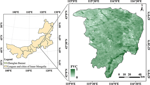
Zhenglan Banner (115° 00′ − 116° 42′ E, 41° 56′ − 43° 11′ N) is situated in the southern part of XilinGol League in Inner Mongolia, within the Otindag sandy land hinterland (Figure 1). The region covers a total area of approximately 10,182 km². Zhenglan Banner exhibits two distinct topographical types: Otindag sandy land and low hills, with an average elevation of 1300 m. It falls under the mid-temperate continental monsoon climate category, characterized by an average annual temperature of 1.5°C and an average annual rainfall of 362.5 mm, mostly concentrated from June to September. The average snow period in the winter lasts around 180 days. Herbaceous vegetation represents a valuable resource in Zhenglan Banner, with the available grassland area accounting for 86.88% of the total land area. Due to variations in moisture, topography, and soil conditions, herbaceous vegetation types can be broadly classified into three main categories: meadow vegetation, typical grassland vegetation, and sand vegetation (Ding et al. 2005). Being the nearest area of typical grassland and sand source to Beijing and Tianjin, Zhenglan Banner’s ecological status holds significant importance. In recent years, the region has implemented various projects such as “Beijing-Tianjin Sandstorm Source Control,” “Returning Grazing Land to Grassland,” “Reclamation of Grasslands in the Agricultural-pastoral Staggered Zone,” and “Grassland Ecological Compensation and Reward.” These national initiatives focused on grassland protection and construction, resulting in substantial improvements in the regional ecological environment (Sun et al. 2019).

Figure 1. Location of the study area (Fraction of Vegetation Coverage (FVC) data is obtained from https://land.copernicus.eu/global/products/fcover).

2.2. Data and preprocessing

2.2.1. Remote sensing data

The remote sensing data used in this study mainly came from Sentinel-1 (S1) and Sentinel-2 (S2), which are provided by ESA and can be accessed through the following link: https://scihub.copernicus.eu/dhus/#/home. S1 is equipped with a C-band SAR sensor capable of acquiring multipolarized SAR data. For this study, we utilized the ground distance format (GRD) image from its IW mode Level 1 product (Level-1), and the downloaded image data were visualized at a resolution of 10 × 10 m. Data preprocessing was performed using the SNAP software platform developed by ESA, which included applying orbit data, radiation calibration, filtering processing, terrain correction, and band synthesis. S2 consists of multispectral optical data with 13 bands and spatial resolutions of 10, 20, and 60 m. The L1C-level data were freely downloaded from the ESA website, and the L2A-level data for research purposes were generated using the Sen2Cor plugin published by ESA (Müller-Wilm 2016). Both the multitemporal S1 and S2 data covered three different seasons: spring, summer, and autumn.

2.2.2. Sample data for grassland type classification

Sample point data were obtained through field surveys conducted from 10 August to 18 August, as well as visual interpretation of multitemporal GF-2 satellite multispectral data and submeter resolution images from Google Earth. The temporal phases of the GF-2 data and Google Earth data corresponded to the peak growing season (June–August), aligning with the field survey data and facilitating accurate determination of grassland types at the sample points. A total of 467 sample points were collected, which were divided into training samples and validation samples in a 7:3 ratio, as detailed in Table 1 and Figure 2. Each sample point represented a range of 2 × 2 pixels, covering an area of 400 km² and providing information about the grassland type within that square region.

Figure 2. Spatial distribution of samples for grassland classification (the background map is from MOD09A1 product (https://ladsweb.modaps.eosdis.nasa.gov/), and the acquisition time is July 2020).

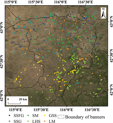
Table 1. Sample information for grassland type classification.

Grassland type	Number of classified samples	Number of validation samples	Total number of samples
Sandy sparse forest grassland	47	19	66
Sandy shrub grassland	61	26	87
Sandy meadow	63	27	90
Low hill steppe	57	24	81
gently sloping steppe	49	21	70
Lowland meadows	52	21	73

3. Method

This section presents a method for achieving refined grassland type identification using multisource and multitemporal active-passive cooperative remote sensing data, employing superpixel image segmentation and random forest classification (Figure 3). The method consists of three main steps:

1. Acquisition of classification features, which includes extracting spectral features from multi-seasonal Sentinel-2 MSI multispectral images, capturing polarization features from multi-seasonal Sentinel-1 C-SAR data, and utilizing eight characteristic parameters representing the full cycle of vegetation growth.

2. Acquisition of geographic object units based on the SLIC0 superpixel algorithm.

3. Utilization of the random forest algorithm and characteristic data at the geographic object-level to identify grassland types, followed by verification of the classification accuracy using a confusion matrix.

Figure 3. Flow chart of grassland classification method.

3.1. Remote sensing-based grassland classification system in Zhenglan Banner

The zonal grassland type in Zhenglan Banner primarily consists of warm typical grassland vegetation with meadow vegetation, whereas the northern sandy area is predominantly occupied by cryptic sandy vegetation. In the sandy vegetation region, the surface landscape exhibits a combination of sand dunes and inter-dune lowlands, forming a regular interlacing pattern. The variations in water and nutrient conditions resulting from this surface landscape contribute to the diversity and complex distribution of sandy vegetation types. At the landscape scale or smaller, topography and soil physicochemical properties are the main factors influencing the distribution pattern of grassland types, as they affect soil water availability. To ensure the rational utilization and protection of sandy vegetation resources, it becomes necessary to further classify sandy grassland types based on microtopographic landforms, vegetation types, and structures.

Although the terrestrial grassland type of typical grassland has a relatively small area share, the herbaceous vegetation in these areas exhibits higher productivity and economic performance, making it crucial for livestock development. However, due to the heterogeneity of regional water and heat, as well as human interference, typical grassland areas also exhibit diverse distributions of grassland types. Decoding and subdividing this information directly from remote sensing imagery is challenging. To achieve a more detailed classification of grassland types in typical grassland areas, it is necessary to consider topographic and geomorphological features, as well as grassland phenological characteristics.

Based on the aforementioned classification criteria for grassland types, and considering the suitability of medium spatial resolution remote sensing images and their practical applications in grassland management, this study adopts the vegetation-habitat classification method. The study mainly draws upon the “comprehensive classification method of occurrence management subject characteristics” developed by Xu et al. (2000), as well as the grassland classification system of Su (1996) in the “1:1000000 China Grassland Resource Map.” Additionally, the research incorporates field survey data on grassland vegetation types in the study area and relevant data on livestock management. As a result, a relatively suitable grassland remote sensing classification system is developed. At the first level, the system primarily reflects soil texture, encompassing three grassland classes: sandy grassland, typical grassland, and meadow. At the second level, the system further delineates the heterogeneous characteristics within different grassland classes, consisting of six grassland subcategories: sandy sparse forest grassland, sandy shrub grassland, sandy meadow, low hill steppe, gently sloping steppe, and lowland meadow (Table 2).

Table 2. Grassland remote sensing classification system.

Level 1	Level 2	Description	MSI image examples (Standard false color)	Sample plot photos
Sandy grassland	Sandy sparse forest grassland	Elm sparsely forested landscapes with tree depression less than 0.3 and herbaceous cover greater than 5%. In the windward slopes of dunes and flat sandy areas, sandy pioneer plants such as Agriophyllum squarrosum., Salsola collina Pall. and Corispermum mongolicum or Artemisia intramongolica H.C.Fu. are the main building blocks. The image tone is white and the texture is coarse.
	Sandy shrub grassland	Shrubs are dominated by Caragana microphylla Lam. and herbs are mainly established by Polygonum divaricatum, Artemisia intramongolica H.C.Fu and Agropyron mongolicum, etc. The shrub cover is less than 30% and the herb cover is more than 5%. The image tone is greenish-gray with light red and rough texture.
	Sandy meadow	Located in the lowland between sand dunes, with no drifting sand disturbance on the surface, and crust layer developed, stable substrate, good soil moisture and nutrient status, mainly distributing communities such as Stipa krylovii Roshev., Artemisia frigida, Agropyron cristatum, Zornia glochidiata, Leymus secalinus, Carex sp., etc., with herbaceous vegetation coverage more than 5%. The image tone is greenish-gray and uniform, the texture is detailed and smooth.
Typical grassland	Low hill steppe	It is distributed in the low hills between 1250 and 1300 m above sea level. It is dominated by grass grasslands with poor weed species, and the representative establishment species are Stipa krylovii Roshev and Artemisia frigida. The total cover of the grassland is low. The image tone is greenish-gray, with clear boundaries with typical grasslands on gentle ground.
	Gently sloping steppe	It is located on the high plains and in the peripheral areas of the mudflats, and is dominated by grassy grasslands with many mixed grasses, represented by Zornia glochidiata and Stipa grandis. Most of the grassland covers not less than 30%. The image tone is pink, with smooth and fine texture.
Meadow	Lowland meadow	It is found in saline lowlands on river floodplains, wide valley bottoms, inland lake basin margins, and poorly drained lowlands. The vegetation type is mainly mesophytic and wet mesophytic perennial herbaceous plants with dense grasses and little bare ground. The image tone is bright red but uneven, with smooth and fine texture.

3.2. Features acquisition

The presence of spectral similarity among different grassland types introduces considerable uncertainty when distinguishing between them. Additionally, the complexity of grassland landscapes necessitates the utilization of features beyond spectral characteristics to improve classification accuracy. Thus, this study incorporates a combination of spectral features (Reflectance and Normalized Difference Vegetation Index (NDVI) (Rouse et al. 1974)), polarization features, and phenological characteristics for the identification of grassland types (Table 3).

Table 3. Features for grassland types identification.

Type	Variable name	Parameter	Definition or description
Spectral characteristics	Reflectance	B2~B4, B8	S2 MSI data for spring, summer, and autumn time phases
	Vegetation index	NDVI	(B8-B4)/(B8+B4)
Polarization characteristics	Backward scattering coefficient	σ	S1 C-SAR data in spring, summer, and autumn phases for two polarization modes VV and VH under σ
Phenological characteristics	Phenology	Phenological characteristics	SOS, EOS, LOS, POP, PEAK, MAU, MGS, MSP and other eight parameters

3.2.1. Multi-seasonal spectral characteristics and vegetation indices

The spectral features were selected from the S2 MSI spectral bands, including Blue, Green, Red, and Near-Infrared bands at a 10 m resolution. Because grassland vegetation is predominantly covered by snow during the winter, data from three periods, namely spring (April 2020), summer (July 2020), and autumn (September 2020), were utilized to characterize the spectral features of different grassland types in different seasons. Additionally, the widely used vegetation index NDVI was employed to further capture the biophysical characteristics of grassland vegetation.

3.2.2. Multi-seasonal polarization characteristics

Considering the distinct height differences among the main vegetation groups within the grassland types identified by the classification system, this study utilized S1 C-SAR data to extract the intensity of the backscattering coefficient σ (Equation (1)(1) $\mathit{\sigma }=10log\mathit{DN}$(1) ) under different polarization modes (VV and VH) as a polarization feature. Similar to the spectral information, data from three periods, namely spring (April 2020), summer (August 2020), and autumn (October 2020), were employed to characterize the polarization images of different grassland types in different seasons.

(1) $\mathit{\sigma }=10log\mathit{DN}$(1)

where DN represents the digital value of each pixel.

3.2.3. Phenological characteristics

High-resolution NDVI time series with both spatial and temporal information can provide a detailed depiction of the complete vegetation growth cycle, enabling the differentiation of various herbaceous vegetation types (Cai et al. 2020). However, the high-spatial-resolution S2 NDVI data have a long revisit period and are prone to cloud contamination during the growing season. Consequently, they cannot offer the same level of temporal coverage as MOD13Q1 NDVI data from MODIS (Moderate Resolution Imaging Spectroradiometer), which hinders a comprehensive representation of the entire vegetation growth cycle using only three seasonal phases of multispectral data. To address the significant spatial and temporal heterogeneity of grasslands and accurately capture the physical and typological changes of different grassland types, this study adopted the STNLFFM model proposed by Cheng et al. (2017). It selected the 23-period MOD13Q1 NDVI data and the S2 MSI NDVI data from three seasonal phases in 2020 as a reference, thereby constructing a high-resolution NDVI time-series dataset for 2020 (with a temporal resolution of 16 d and a spatial resolution of 10 m). Subsequently, the dataset was interpolated to a daily scale to facilitate vegetation phenology feature extraction.

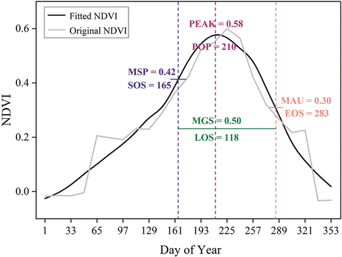
For grassland vegetation type identification, eight phenological characteristics were selected, including start of the season (SOS), end of the season (EOS), length of the season (LOS), position of peak value (POP), peak value (PEAK), mean autumn value (MAU), mean growing season value (MGS), and mean spring value (MSP). These characteristics were chosen based on previous studies (Cai, Lin, and Zhang 2019; Zhang et al. 2018) (Figure 4). SOS and EOS represent the dates when the NDVI exhibits the fastest increase and decrease at the daily scale, respectively. LOS is the duration between SOS and EOS. MGS can be calculated based on LOS. POP and PEAK correspond to specific points in the growth cycle. MAU and MGS are derived from the season length, and their calculation method is described in detail in the following main steps. Further information about the phenological characteristics can be found in Forkel et al. (2015).

Figure 4. Phenological characteristics obtained using the extreme value method based on the first derivative of the NDVI time series. This example illustrates the eight phenological characteristics based on the variation curves of NDVI over a year. The black line represents the curve of NDVI interpolated to the daily scale, whereas the gray line represents the curve of MODIS NDVI. The values for MSP, MAU, PEAK, and MGS are 0.42, 0.30, 0.58, and 0.50, respectively, whereas SOS, EOS, POP, and LOS are represented on the X-axis as the day of the year, with values of 165, 283, 210, and 118, respectively. All phenological characteristics are categorized into four groups: MSP&SOS, MAU&EOS, MGS&LOS, and PEAK&POP, and they are appropriately marked in the figure.

The process of extracting phenological characteristics involves three main steps:

1. A cubic spline approach was applied to smooth and interpolate the 23-period high-resolution NDVI time-series data for 2020 to obtain daily-scale data (Migliavacca et al. 2011).

2. Seasonality check was conducted on the smoothed and interpolated NDVI time series. Three seasonality checking methods were employed: the periodogram method (Ripley 2002), autocorrelation function method (Ripley 2002), and the seasonal trend model. To ensure accuracy, seasonality was assigned to the time series only when all three methods indicated its presence. If one or more methods indicated no seasonality, only POP and PEAK, which do not depend on SOS and EOS estimates, were calculated.

3. The phenological parameters SOS and EOS were determined by identifying the extreme values of the first-order derivatives of the NDVI time series in the presence of seasonality (Tateishi and Ebata 2004).

3.3. Object-oriented classification

3.3.1. Image segmentation

Image segmentation plays a crucial role in object-oriented classification (Hossain and Chen 2019) and is a critical step in geographic object-based image analysis (GEOBIA). The quality of image segmentation directly affects the final feature extraction and classification accuracy. Studies have demonstrated (Csillik 2017; Ortiz Toro et al. 2015) that the SLIC superpixel segmentation algorithm outperforms other traditional methods in terms of geometric accuracy and computational efficiency when applied to natural scenes (Csillik 2017). The SLIC algorithm is an adaptive k-means clustering algorithm that requires three main parameters: the initial clustering center distance (S) and the number of clustering iterations (I) determine the number of generated superpixels of the same size, whereas the compactness (m) controls their compactness. In this study, the S parameter is set to 10 × 10 as the initial size, and the number of iterations is set to 10 (Achanta et al. 2012). To generate regularly shaped superpixels in both textured and non-textured regions of the image, the SLIC0 algorithm proposed by Achanta et al. (2012) is utilized, which does not require determining the m parameter. SLIC0 can adaptively select the optimal compactness parameter for each superpixel. Therefore, in this study, the S2 MSI data from three quarters are fused as the image layer, and the SLIC0 superpixel algorithm (Achanta et al. 2012) is employed to generate regular-shaped superpixels by perceptually grouping pixels with similar features.

3.3.2. Random forest classification

The random forest algorithm is a versatile machine learning algorithm used for classification and regression tasks (Breiman 2001). It offers advantages such as high classification accuracy, stable classification results, and fast processing speed in high-dimensional data classification. It is widely used in the study of remote sensing classification (Belgiu and Drăguţ 2016), even in combination with hyperpixels for GEOBIA (Kawamura et al. 2021). It has been widely used in the research of remote sensing classification, and there are also related researches to combine it with hyperpixel to realize GEOBIA classification.

When using the random forest model, the key parameters to be controlled are the number of decision trees (ntree) and the number of variables used for building individual trees (mtry). In this study, the range of values for each parameter was tested independently, and the corresponding classification accuracy was calculated using the cross-validation method. The optimal values for both parameters were determined based on the overall classification accuracy. It was found that when mtry = 6 and ntree = 1500, all classification tasks based on different feature combinations consistently achieved the highest overall accuracy, representing the optimal classification results.

3.4. Classification accuracy evaluation

In this study, validation sample points were employed to calculate the corresponding confusion matrix and conduct a quantitative evaluation of the accuracy of both pixel-based and object-oriented classification methods. This evaluation involved calculating Production Accuracy (PA), User Accuracy (UA), Overall Accuracy (OA), and Kappa coefficient as metrics to summarize the classification performance.

4. Results and Analysis

4.1. Spatiotemporal fusion effect and phenological characteristic extraction

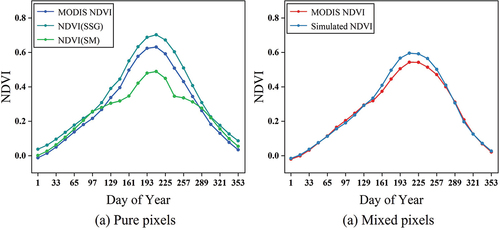
In this study, a comparison was made between the time-series variation of MOD13Q1 NDVI products and the constructed high-spatial-resolution NDVI data for both pure and mixed pixels. Figure 5 illustrates that for pure pixels, there is only a minor discrepancy between the MOD13Q1 NDVI time series and the simulated NDVI time series. However, in the case of mixed pixels in which two different grassland types are present within the same MOD13Q1 pixel, the MOD13Q1 NDVI time series aligns more closely with the NDVI time profile of sandy scrub and fails to capture the distribution of sandy meadows. On the other hand, the high-spatial-resolution NDVI generated by STNLFFM successfully captures the NDVI time profiles of both grassland types. These findings effectively demonstrate that the utilization of NDVI time series to extract the variations in vegetation phenology among different grassland types can aid in defining the transitional boundaries of the six grassland types.

Figure 5. Comparison of fused NDVI time series with MODIS NDVI time series for pure pixel (a) and mixed pixel(b).

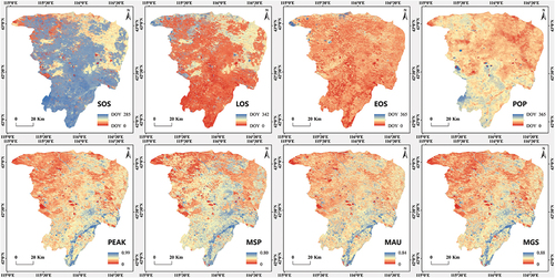
Additionally, the high-resolution NDVI time-series data were spatially interpolated to a daily scale. Subsequently, using the grassland vegetation phenological characteristic extraction method described in Section 2.2 (refer to Figure 6), eight phenological characteristics were derived. These characteristics include SOS, EOS, LOS, PEAK, POP, MSP, MAU, and MGS. By integrating these phenological characteristics with the field survey data of grassland types, it was observed that the six grassland types exhibited distinct spatial variations in their phenological periods. The extraction of phenological characteristics based on vegetation growth patterns proves to be valuable for the accurate identification of grassland types.

Figure 6. Eight phenological characteristics extracted based on the fused NDVI time series.

4.2. Influence of fusing different classification features on classification accuracy

We employed an object-oriented approach to extract grassland type information using four feature combinations: multi-seasonal spectral features, multi-seasonal spectral features with polarization features, multi-seasonal spectral features with phenology features, and a combination of all three features as input. The extraction results are presented in Table 4 and Figure 7. The results demonstrate that the classification method combining multi-seasonal spectral, polarization, and phenology features achieves the highest classification accuracy, with an OA of 82.61% and a kappa coefficient of 0.79. Compared to using only multi-seasonal spectral features, this approach improves the accuracy by 15.94% and the kappa coefficient by 0.19, indicating significant overall improvement. The inclusion of polarization and phenological characteristics individually also leads to notable enhancements in classification accuracy. Specifically, the addition of polarization information improves accuracy by 13.76% and the kappa coefficient by 0.16, whereas the addition of phenological characteristics improves accuracy by 9.42% and the kappa coefficient by 0.11.

Figure 7. UA and PA of the six grassland types with different feature combinations.

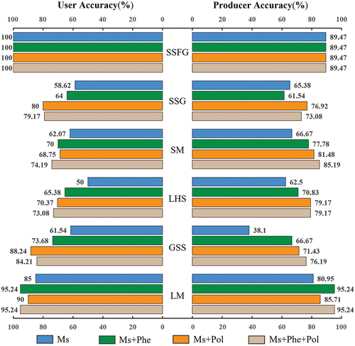
Table 4. Classification accuracy of different feature combinations.

Combination method	Multi-seasonal spectral characteristics	Multi-seasonal spectral + Phenological characteristics	Multi-seasonal spectral + Polarization characteristics	Multi-seasonal spectral + Phenological + Polarization characteristics
OA (%)	66.67	76.09	8.43	82.61
Kappa coefficient	.5975	.7117	.7639	.7903

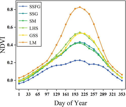
Among the various grassland types, sandy sparse forest grasslands consistently exhibit the best performance across different classification schemes. The use of multi-seasonal spectral information contributes to a more favorable recognition effect for this type, mainly because it is predominantly characterized by elm sparse forest landscapes, which exhibit distinct seasonal differences compared with other grassland types dominated by herbs and shrubs. In the identification of sandy scrub, the inclusion of polarization features significantly improves classification accuracy compared to phenological characteristics. This improvement may be attributed to the fact that sandy scrub, with its shrub vegetation characteristics and relatively small intra-annual growth variation, exhibits greater sensitivity to the geometric features captured by SAR data. Sandy scrub is prone to misclassification with sandy meadow and low hill steppe, particularly evident from the confusion matrix. The annual NDVI variation of sandy scrub is relatively flat and falls within the midrange of the six types, making it susceptible to misclassification with these two types (Figure 8).

Figure 8. NDVI time series of six grassland types.

Conversely, for the lowland meadow type, phenological information demonstrates a distinct advantage, resulting in a mapping accuracy of 95.24%, nearly 15% higher than the accuracy achieved by the multi-seasonal spectral feature extraction method. The performance of polarization information is generally average for this type, mainly because it is predominantly found in lowland areas in which SAR data’s backward scattering coefficient shows low sensitivity to geometric features. The pronounced growth cycle characteristics of herbaceous vegetation in lowland meadows facilitate easier differentiation. For the remaining three types, namely sandy meadow, low hill steppe, and gently sloping steppe, the inclusion of polarization features or phenological characteristics leads to improved classification accuracy, particularly notable in the case of gently sloping steppe, in which recognition accuracy improves by approximately 30%–40%. In conclusion, combining multi-seasonal spectral features with polarization and phenology features significantly enhances the classification accuracy of grassland types.

4.3. Spatial distribution pattern of grassland types in Zhenglan Banner

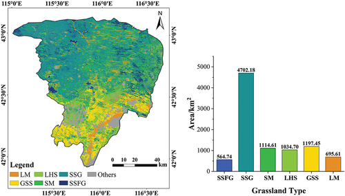
The OA of grassland type recognition in Zhenglan Banner reached 82.61%, and the resulting spatial distribution of the different grassland types is illustrated in Figure 9. Analysis of the grassland classification results for the Zhenglan Banner in 2020 revealed that grassland dominates the region, covering a total area of 9309.29 km², which accounts for 91.43% of the entire area. Moving from north to south, the sequence of grassland types is sandy grassland followed by typical grassland. Sandy grassland is the largest type, spanning a total area of 6381.53 km², consisting of 564.74 km² of sandy sparse forest grassland, 4702.18 km² of sandy shrub grassland, and 1114.61 km² of sandy meadow. Typical grassland covers an area of 2232.15 km², with 1034.70 km² located in gently sloping areas and 1197.45 km² in low hills. Lowland meadows, characterized as cryptogamic vegetation, are primarily situated in low-lying areas and floodplains in which surface runoff accumulates in the southeast and north-central parts of the Zhenglan Banner, occupying an area of 695.61 km².

Figure 9. Grassland type classification result in Zhenglan Banner.

4.4. Differences in phenological growth of various types of grassland in Zhenglan Banner

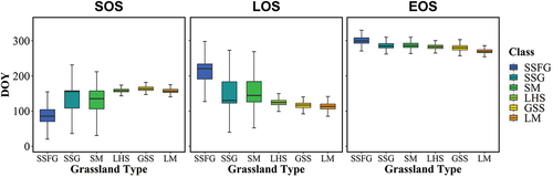
Combining the spatial distribution of grassland types in Zhenglan Banner, we conducted a further analysis of the variations in phenological growth characteristics among different grassland types. As shown in Figure 10, each grassland type exhibits distinct phenological periods, with sandy grassland having a considerably longer growing season compared with typical grassland and meadow. For instance, sandy sparse forest grassland has the longest growing season length, spanning 215 days (from day 85 to day 300), whereas lowland meadow has the shortest growing season, lasting only 113 days (from day 156 to day 269). Overall, the vegetation growth cycle is predominantly concentrated between May and September. Sandy sparse forest grassland experiences the earliest onset of the growing season, sprouting by the end of March (day 85), whereas gently sloping steppe has the latest start date, typically around mid-early June (day 163). In contrast, lowland meadows exhibit the earliest end date for the growing season, concluding in early September (day 269). These distinct phenological growth patterns serve as valuable indicators for accurately identifying each grassland type.

Figure 10. Box plots of phenological characteristics of different grassland types.

5. Discussion

5.1. Construction of grassland remote sensing classification system

Various regions around the world have developed distinct grassland classification systems based on their economic and ecological conditions. These systems can be broadly categorized into seven major types: plant topography, phytocoenology, agricultural management, land-botany, climatology-botany, vegetation-habitat, and integrated climate-land-vegetation order (Liang et al. 2011). The Chinese grassland type classification system, based on land-botany theory, includes two main systems: the grassland comprehensive sequential classification system (Hu 1997; Ren 2008; Ren et al. 1980) and the vegetation-habitat classification system of grassland (VHCS) (Chen et al. 2002; Jia 1980; Xu, Hu, and Zhu 2000; Zhang 1988).

With advancements in remote sensing and spatial analysis techniques, grassland type classification has evolved to incorporate data from multiple sources, emphasizing intuition and visualization. Consequently, it is necessary to develop a remote sensing classification system for grasslands by harnessing the observation capabilities of remote sensing technology. However, there is a dearth of detailed studies on remote sensing classification systems for grasslands, necessitating the integration of rich a priori knowledge. In this study, we explore the construction of a remote sensing classification system for grasslands based on vegetation-habitat taxonomy and combined it with the observation capabilities of S2 data. Although the system is representative to some extent, further additions and trade-offs are necessary to align with grassland regulation objectives, geographical characteristics, and the spatial resolution of remote sensing data.

5.2. Use of remote sensing data

This study capitalizes on the data advantage offered by active-passive remote sensing synergy. Multispectral data are the most commonly used remote sensing data, whereas C-band SAR data, with their limited penetration capability compared with L-band SAR data, are employed for SAR analysis due to data acquisition constraints. SAR data such as S1 and GF-3, which are more readily available, are predominantly C-SAR data, and the application potential of other band data requires further exploration. Additionally, studies have shown that high-spatial-resolution visible data acquired by near-earth UAVs can effectively facilitate grassland species identification (Crabbe, Lamb, and Edwards 2019; Golzarian and Frick 2011; Hung, Xu, and Sukkarieh 2014). However, data acquisition limitations hinder their large-scale application. Hyperspectral data, with their greater spectral information compared with multispectral data, demonstrate advantages in extracting vegetation biochemical indicators, such as chlorophyll content. Initial applications have been made in grassland type identification and studies on grassland species diversity (Bao et al. 2017; Peng et al. 2018; Skidmore et al. 2010). Nevertheless, the periodic revisit of hyperspectral data and limited frequency pose challenges for broader spatial applications. Currently, multispectral data remain the primary data source for grassland type identification. However, a single remote sensing data source cannot provide the required spectral, spatial, and temporal information simultaneously. Furthermore, remote sensing data alone may not sufficiently capture vegetation growth habits and environmental characteristics. Consequently, integrating multisource data observations, including SAR, UAV, hyperspectral, and LiDAR data, present a crucial direction for enhancing the fine identification of grassland types.

5.3. Application of remote sensing features for grassland type identification

This study reveals that fusing multispectral features, polarization features, and phenological characteristics enhances the refinement level and classification accuracy of grassland type identification. Polarization characteristics reflect differences in vertical structure; however, considering the relatively low vegetation and high soil noise in grasslands, further research is required to determine optimal applications of polarization characteristics. Some studies have indicated the beneficial role of physical characteristics in improving the accuracy of grassland type identification (Cai et al. 2020; Lindsay et al. 2018; Qu et al. 2021). The phenological characteristics extraction method proposed in this study captures the key points of vegetation growth changes within a year more accurately, thereby contributing to grassland type identification. Additionally, certain spectral bands, such as near-infrared, mid-infrared, and thermal infrared, have been shown to facilitate plant species differentiation (Csillik 2017). Texture feature grayscale co-occurrence matrices are often employed as auxiliary features to spectral features, which can enhance the accuracy of vegetation type classification to some extent (Cao et al. 2018; Yang, Smith, and Hill 2017). Incorporating non-remote sensing information like topography and soil can effectively enhance the separability of grassland types and improve classification accuracy (Ma 2015; Xu 2019). However, the inclusion of additional features may introduce challenges such as feature redundancy, placing higher demands on classification methods, and necessitating considerations of data matching in spatial and temporal dimensions. Nonetheless, it is evident that utilizing multisource features will be an effective approach to achieve refined recognition of grassland types.

5.4. Refinement of grassland type identification

Most studies based on remote-sensing data for grassland type identification exhibit a low degree of classification refinement (Parente et al. 2019; Schwieder et al. 2016; Shen et al. 2016). Xu (2019) utilized Landsat time-series data to classify land cover in the Hulunbuir grassland in China, achieving an overall classification accuracy of 94.41%. However, the primary focus was on distinguishing between meadow grassland and typical grassland. Conversely, Crabbe et al. (2019) classified grassland types based on species composition complexity, distinguishing between three main grassland categories: single-species, two-species, and multispecies. The OA, based on the combined S1 and S2 data, reached 96%. This demonstrates that classification accuracy tends to be higher when the degree of classification refinement is lower. Research on more refined grassland type identification is limited, as exemplified by this paper’s subdivision of grassland types into six categories with an OA of 82.61%. Rapinel et al. (2020) conducted a more refined vegetation type identification in the Mediterranean region using MODIS time-series data, achieving an overall classification accuracy of 76%. Currently, research on the identification of grassland types with higher degrees of refinement exhibits relatively lower accuracy, suggesting that this field is still in the exploratory stage. Future research should delve deeper into data and classification methods to enhance classification accuracy in this area.

6. Conclusions

The conclusions of this study are as follows:

1. This study addresses the application needs of grassland resource regulation and proposes a grassland remote sensing classification system suitable for the northern natural grassland. Based on the vegetation-habitat classification method and the separability of remote sensing, the system divides the grassland into three primary categories (sandy grassland, typical grassland, and meadow) and further subdivides them into six secondary categories (sandy sparse forest grassland, sandy shrub grassland, sandy meadow, low hill steppe, gently sloping steppe, and lowland meadow). This classification system can serve as a reference for constructing remote sensing fine identification systems for natural grasslands in other regions.

2. By leveraging S2’s advantage of high spatial resolution and the temporal resolution advantage of MODIS NDVI products, this study generates high-spatial-resolution NDVI using the STNLFFM method. This NDVI captures the temporal profile of grassland types and enables the accurate extraction of vegetation phenological information, particularly in mixed pixels. The method accurately reflects the changing characteristics of different grassland types at various growth stages, facilitating fine identification.

3. Under the object-oriented framework, this study utilizes SLIC0 superpixel segmentation and random classification for the fine identification of grassland types. The classification method that integrates multi-seasonal phase spectrum, polarization, and phenological characteristics achieves the highest classification effectiveness. The OA reaches 82.61%, with a kappa coefficient of 0.79. This is a significant improvement compared with the classification method that only uses multi-seasonal phase spectrum, increasing the kappa coefficient by 0.19 and improving the overall classification effect. The inclusion of separate polarization features and phenological characteristics enhances the classification accuracy by 13.76% and 9.42%, respectively. The polarization features contribute the most to the identification of sandy scrub, whereas phenological characteristics exhibit a clear advantage in identifying lowland meadow types, achieving a mapping accuracy of 95.24%. The sandy sparse forest grassland is the easiest to identify among the six types, and the identification accuracy of typical grassland in gentle land significantly improves. In general, the use of polarization or phenological information enhances the extraction accuracy by approximately 30%–40%.

4. The Zhenglan Banner is predominantly covered by grassland, encompassing a total area of 9309.29 km², accounting for 91.43% of the region’s area. Among the grassland types, sandy grassland is the largest, covering a total area of 6381.53 km². Analysis of phenological characteristics reveals that the growth cycle of grassland vegetation is concentrated in May–September. Sandy grassland exhibits a significantly longer growing season compared with typical grassland and meadow. The growing season length ranges from 215 days for sandy sparse forest grassland to only 113 days for lowland meadow. These distinct phenological characteristics facilitate the accurate identification of each grassland type.

Disclosure statement

No potential conflict of interest was reported by the author(s).

Data availability statement

Due to confidentiality agreements, supporting data can only be made available to bona fide researchers subject to a nondisclosure agreement. Details of the data and how to request access are available from Dr. Bin Sun at the Institute of Forest Resource Information Techniques, Chinese Academy of Forestry.

Additional information

Funding

This work was supported by the National Natural Science Foundation of China [grant number 42001386; 42271407] and within the ESA-MOST China Dragon 5 Cooperation (ID:59313).

Notes on contributors

Bin Sun

Bin Sun received the PhD degree in forest management from the Chinese Academy of Forestry in 2016. He is an associate professor at the Institute of Forest Resource Information Techniques, Chinese Academy of Forestry. His research interests include remote sensing monitoring and assessment of desertification and grasslands.

Pengyao Qin

Pengyao Qin received the PhD degree in forest management from the Chinese Academy of Forestry in 2022. His research interests include remote sensing technology and applications for grasslands.

Changlong Li

Changlong Li is a lecturer in the School of Information Technology and Engineering, Guangzhou College of Commerce. His research interests include remote sensing technology and applications.

Zhihai Gao

Zhihai Gao received the PhD degree from Beijing Forestry University in 2003. He is a professor at the Institute of Forest Resource Information Techniques, Chinese Academy of Forestry. His research interests include remote sensing monitoring and assessment of desertification and land degradation.

Alan Grainger

Alan Grainger is a professor at the University of Leeds. His research interests include modeling global environmental change and desertification.

Xiaosong Li

Xiaosong Li received the PhD degree from the Chinese Academy of Forestry in 2008. His research interests include remote sensing big data and sustainability.

Yan Wang

Yan Wang received the Master’s degree from the Chinese Academy of Forestry in 2018. Her research interests include remote sensing technology and applications for Arid/Semi-arid area.

Wei Yue

Wei Yue is currently working toward the PhD degree at the Institute of Forest Resource Information Techniques, Chinese Academy of Forestry. His research interests include remote sensing technology and applications for forests and grasslands.

References

- Achanta, R., A. Shaji, K. Smith, A. Lucchi, P. Fua, and S. Süsstrunk. 2012. “SLIC Superpixels Compared to State-Of-The-Art Superpixel Methods.” IEEE Transactions on Pattern Analysis and Machine Intelligence 34 (11): 2274–2282. https://doi.org/10.1109/TPAMI.2012.120.
- Anderson, J. R., E. E. Hardy, J. T. Roach, and R. E. Witmer. 1976. “Professional Paper.” US Geological Survey: Reston, VA, USA.
- Bao, S. N., C. X. Cao, W. Chen, and H. J. Tian. 2017. “Spectral Features and Separability of Alpine Wetland Grass Species.” Spectroscopy Letters 50 (5): 245–256. https://doi.org/10.1080/00387010.2016.1240088.
- Bartholome, E., and A. S. Belward. 2005. “GLC2000: A New Approach to Global Land Cover Mapping from Earth Observation Data.” International Journal of Remote Sensing 26 (9): 1959–1977. https://doi.org/10.1080/01431160412331291297.
- Belgiu, M., and L. Drăguţ. 2016. “Random Forest in Remote Sensing: A Review of Applications and Future Directions.” ISPRS Journal of Photogrammetry and Remote Sensing 114:24–31. https://doi.org/10.1016/j.isprsjprs.2016.01.011.
- Breiman, L. 2001. “Random Forests.” Machine Learning 45 (1): 5–32. https://doi.org/10.1023/A:1010933404324.
- Bruzzone, L., and L. Carlin. 2006. “A Multilevel Context-Based System for Classification of Very High Spatial Resolution Images.” IEEE Transactions on Geoscience and Remote Sensing 44 (9): 2587–2600. https://doi.org/10.1109/TGRS.2006.875360.
- Cai, Y. T., X. Y. Li, M. Zhang, and H. Lin. 2020. “Mapping Wetland Using the Object-Based Stacked Generalization Method Based on Multi-Temporal Optical and SAR Data.” International Journal of Applied Earth Observation and Geoinformation 92:102164. https://doi.org/10.1016/j.jag.2020.102164.
- Cai, Y. T., H. Lin, and M. Zhang. 2019. “Mapping Paddy Rice by the Object-Based Random Forest Method Using Time Series Sentinel-1/sentinel-2 Data.” Advances in Space Research 64 (11): 2233–2244. https://doi.org/10.1016/j.asr.2019.08.042.
- Cao, J. J., W. C. Leng, K. Liu, L. Liu, Z. He, and Y. H. Zhu. 2018. “Object-Based Mangrove Species Classification Using Unmanned Aerial Vehicle Hyperspectral Images and Digital Surface Models.” Remote Sensing 10 (1): 89. https://doi.org/10.3390/rs10010089.
- Chen, Z. Z., Y. F. Wang, S. P. Wang, and X. M. Zhou. 2002. “Preliminary Studies on the Classification of Grassland Ecosystem in China.” Acta Agrestia Sinica 10 (2): 81. ( In Chinese).
- Cheng, Q., H. Liu, H. Shen, P. Wu, and L. Zhang. 2017. “A spatial and temporal nonlocal filter-based data fusion method.” IEEE Transactions on Geoscience & Remote Sensing 55 (8): 4476–4488. https://doi.org/10.1109/TGRS.2017.2692802.
- Crabbe, R. A., D. Lamb, and C. Edwards. 2019. “Discrimination of Species Composition Types of a Grazed Pasture Landscape Using Sentinel-1 and Sentinel-2 Data.” International Journal of Applied Earth Observation and Geoinformation 84:101978. https://doi.org/10.1016/j.jag.2019.101978.
- Csillik, O. 2017. “Fast Segmentation and Classification of Very High Resolution Remote Sensing Data Using SLIC Superpixels.” Remote Sensing 9 (3): 243. https://doi.org/10.3390/rs9030243.
- Ding, G. D., S. Y. Li, J. Y. Cai, T. N. Zhao, X. Wang, and X. Ling. 2005. “Pasture Resources Evaluation and Stocking Density in Hunshandake Sandy Land: Case Study of Zhenglan Banner, Inner Mongolia.” Chinese Journal of Ecology 9:1038. https://doi.org/10.13292/j.1000-4890.2005.0095.
- Fisher, P. 1997. “The Pixel: A Snare and a Delusion.” International Journal of Remote Sensing 18 (3): 679–685. https://doi.org/10.1080/014311697219015.
- Forkel, M., M. Migliavacca, K. Thonicke, M. Reichstein, S. Schaphoff, U. Weber, and N. Carvalhais. 2015. “Codominant Water Control on Global Interannual Variability and Trends in Land Surface Phenology and Greenness.” Global Change Biology 21 (9): 3414–3435. https://doi.org/10.1111/gcb.12950.
- Gilbertson, J. K., J. Kemp, and A. V. Niekerk. 2017. “Effect of Pan-Sharpening Multi-Temporal Landsat 8 Imagery for Crop Type Differentiation Using Different Classification Techniques.” Computers and Electronics in Agriculture 134:151–159. https://doi.org/10.1016/j.compag.2016.12.006.
- Golzarian, M. R., and R. A. Frick. 2011. “Classification of Images of Wheat, Ryegrass and Brome Grass Species at Early Growth Stages Using Principal Component Analysis.” Plant Methods 7 (1): 1–11. https://doi.org/10.1186/1746-4811-7-28.
- Gómez, C., J. C. White, and M. A. Wulder. 2016. “Optical Remotely Sensed Time Series Data for Land Cover Classification: A Review.” ISPRS Journal of Photogrammetry and Remote Sensing 116:55–72. https://doi.org/10.1016/j.isprsjprs.2016.03.008.
- Hossain, M. D., and D. M. Chen. 2019. “Segmentation for Object-Based Image Analysis (OBIA): A Review of Algorithms and Challenges from Remote Sensing Perspective.” ISPRS Journal of Photogrammetry and Remote Sensing 150:115–134. https://doi.org/10.1016/j.isprsjprs.2019.02.009.
- Hu, Z. Z. 1997. Introduction to Prairie Taxonomy. Beijing: China Agriculture Press. ( In Chinese).
- Huang, C., E. L. Geiger, W. J. D. Van Leeuwen, and S. E. Marsh. 2009. “Discrimination of Invaded and Native Species Sites in a Semi-Desert Grassland Using MODIS Multi-Temporal Data.” International Journal of Remote Sensing 30 (4): 897–917. https://doi.org/10.1080/01431160802395243.
- Hung, C., Z. Xu, and S. Sukkarieh. 2014. “Feature Learning Based Approach for Weed Classification Using High Resolution Aerial Images from a Digital Camera Mounted on a UAV.” Remote Sensing 6 (12): 12037–12054. https://doi.org/10.3390/rs61212037.
- Jia, S. X. 1980. “Discussion on the Classification of Grassland Types in China.” Chinese Journal of Grasslands (1):11–13. ( In Chinese).
- Kang, J., X. H. Hou, Z. Niu, S. Gao, and K. Jia. 2014. “Decision Tree Classification Based on Fitted Phenology Parameters from Remotely Sensed Vegetation Data.” Transactions of the Chinese Society of Agricultural Engineering 30 (9): 148–156. https://doi.org/10.3969/j.issn.1002-6819.2014.09.019.
- Kaszta, Ż., R. V. D. Kerchove, A. Ramoelo, M. A. Cho, S. Madonsela, R. Mathieu, and E. Wolff. 2016. “Seasonal Separation of African Savanna Components Using Worldview-2 Imagery: A Comparison of Pixel-And Object-Based Approaches and Selected Classification Algorithms.” Remote Sensing 8 (9): 763. https://doi.org/10.3390/rs8090763.
- Kawamura, K., H. Asai, T. Yasuda, P. Soisouvanh, and S. Phongchanmixay. 2021. “Discriminating Crops/Weeds in an Upland Rice Field from UAV Images with the SLIC-RF Algorithm.” Plant Production Science 24 (2): 198–215. https://doi.org/10.1080/1343943X.2020.1829490.
- Liang, T. G., Q. S. Feng, X. D. Huang, and J. Z. Ren. 2011. “Review in the Study of Comprehensive Sequential Classification System of Grassland.” Acta Prataculturae Sinica 20 (5): 252. ( In Chinese).
- Lindsay, E. J., D. J. King, A. M. Davidson, and B. Daneshfar. 2018. “Canadian Prairie Rangeland and Seeded Forage Classification Using Multiseason Landsat 8 and Summer RADARSAT-2.” Rangeland Ecology & Management 72 (1): 92–102. https://doi.org/10.1016/j.rama.2018.07.005.
- Liu, M., L. Dries, J. K. Huang, S. Min, and J. J. Tang. 2019. “The Impacts of the Eco-Environmental Policy on Grassland Degradation and Livestock Production in Inner Mongolia, China: An Empirical Analysis Based on the Simultaneous Equation Model.” Land Use Policy 88:104167. https://doi.org/10.1016/j.landusepol.2019.104167.
- Loveland, T. R., B. C. Reed, J. F. Brown, D. O. Ohlen, Z. Zhu, L. Yang, and J. W. Merchant. 2000. “Development of a Global Land Cover Characteristics Database and IGBP DISCover from 1 Km AVHRR Data.” International Journal of Remote Sensing 21 (6–7): 1303–1330. https://doi.org/10.1080/014311600210191.
- Ma, W. W. 2015. “Study on Methods for Grassland Classification and Quality Estimation by Remote Sensing: A Case Study in the Region around Qinghai Lake.” PhD diss., University of Chinese Academy of Sciences.
- Mao, D., Z. M. Wang, B. J. Du, L. Li, Y. L. Tian, M. M. Jia, Y. Zeng, K. S. Song, M. Jiang, and Y. Q. Wang. 2020. “National Wetland Mapping in China: A New Product Resulting from Object-Based and Hierarchical Classification of Landsat 8 OLI Images.” ISPRS Journal of Photogrammetry and Remote Sensing 164:11–25. https://doi.org/10.1016/j.isprsjprs.2020.03.020.
- McInnes, W. S., B. Smith, and G. J. McDermid. 2015. “Discriminating Native and Nonnative Grasses in the Dry Mixedgrass Prairie with MODIS NDVI Time Series.” IEEE Journal of Selected Topics in Applied Earth Observations and Remote Sensing 8 (4): 1395–1403. https://doi.org/10.1109/JSTARS.2015.2416713.
- Migliavacca, M., M. Galvagno, E. Cremonese, M. Rossini, M. Meroni, O. Sonnentag, S. Cogliati, et al. 2011. “Using Digital Repeat Photography and Eddy Covariance Data to Model Grassland Phenology and Photosynthetic CO2 Uptake.” Agricultural and Forest Meteorology 151 (10): 1325–1337. https://doi.org/10.1016/j.agrformet.2011.05.012.
- Ministry of Land and Resources of the People’s Republic of China. 2017. Current Land Use Classification. Beijing: China Quality And Standards Publishing & Media Co., Ltd. ( In Chinese).
- Müller, H., P. Rufin, P. Griffiths, A. J. B. Siqueira, and P. Hostert. 2015. “Mining Dense Landsat Time Series for Separating Cropland and Pasture in a Heterogeneous Brazilian Savanna Landscape.” Remote Sensing of Environment 156:490–499. https://doi.org/10.1016/j.rse.2014.10.014.
- Müller-Wilm, U. 2016. “Sentinel-2 MSI–Level-2A Prototype Processor Installation and User Manual.” Telespazio VEGA Deutschland GmbH: Darmstadt, Germany 51.
- Ortiz Toro, C. A., C. G. Martín, Á. G. Pedrero, and E. M. Ruiz. 2015. “Superpixel-Based Roughness Measure for Multispectral Satellite Image Segmentation.” Remote Sensing 7 (11): 14620–14645. https://doi.org/10.3390/rs71114620.
- Parente, L., V. Mesquita, F. Miziara, L. Baumann, and L. Ferreira. 2019. “Assessing the Pasturelands and Livestock Dynamics in Brazil, from 1985 to 2017: A Novel Approach Based on High Spatial Resolution Imagery and Google Earth Engine Cloud Computing.” Remote Sensing of Environment 232:111301. https://doi.org/10.1016/j.rse.2019.111301.
- Peng, Y., M. Fan, J. Y. Song, T. T. Cui, and R. Li. 2018. “Assessment of Plant Species Diversity Based on Hyperspectral Indices at a Fine Scale.” Scientific Reports 8 (1): 4776. https://doi.org/10.1038/s41598-018-23136-5.
- Qu, L. A., Z. J. Chen, M. C. Li, J. J. Zhi, and H. M. Wang. 2021. “Accuracy Improvements to Pixel-Based and Object-Based Lulc Classification with Auxiliary Datasets from Google Earth Engine.” Remote Sensing 13 (3): 453. https://doi.org/10.3390/RS13030453.
- Rapinel, S., C. Rozo, P. Delbosc, D. Arvor, A. Thomas, J. B. Bouzille, F. Bioret, and L. Hubert-Moy. 2020. “Mapping the Functional Dimension of Vegetation Series in the Mediterranean Region Using Multitemporal MODIS Data.” Giscience & Remote Sensing 57 (1): 60–73. https://doi.org/10.1080/15481603.2019.1662167.
- Ren, J. Z. 2008. “Classification and Cluster Applicable for Grassland Type.” Acta Agrestia Sinica 16 (1): 4. ( In Chinese).
- Ren, J. Z., Z. Z. Hu, X. D. Mou, and P. J. Zhang. 1980. “Comprehensive Sequential Taxonomy of Grasslands and Its Steppegenesis Significance.” Chinese Journal of Grasslands 38 (1): 12–24. ( In Chinese).
- Ren, Y. H., Y. P. Zhu, D. Baldan, M. D. Fu, B. Wang, J. S. Li, and A. Chen. 2021. “Optimizing Livestock Carrying Capacity for Wild Ungulate-Livestock Coexistence in a Qinghai-Tibet Plateau Grassland.” Scientific Reports 11 (1): 3635. https://doi.org/10.1038/s41598-021-83207-y.
- Ripley, B. D. 2002. Modern Applied Statistics with S. New York: Springer.
- Rouse, J. W., R. H. Haas, J. A. Schell, and D. W. Deering. 1974. “Monitoring Vegetation Systems in the Great Plains with ERTS.” NASA Special Publication 351 (1): 309.
- Schwieder, M., P. J. Leitão, M. Bustamante, L. G. Ferreira, A. Rabe, and P. Hostert. 2016. “Mapping Brazilian Savanna Vegetation Gradients with Landsat Time Series.” International Journal of Applied Earth Observation and Geoinformation 52:361–370. https://doi.org/10.1016/j.jag.2016.06.019.
- Senf, C., P. J. Leitão, D. Pflugmacher, S. V. D. Linden, and P. Hostert. 2015. “Mapping Land Cover in Complex Mediterranean Landscapes Using Landsat: Improved Classification Accuracies from Integrating Multi-Seasonal and Synthetic Imagery.” Remote Sensing of Environment 156:527–536. https://doi.org/10.1016/j.rse.2014.10.018.
- Shafizadeh-Moghadam, H., M. Khazaei, S. K. Alavipanah, and Q. H. Weng. 2021. “Google Earth Engine for Large-Scale Land Use and Land Cover Mapping: An Object-Based Classification Approach Using Spectral, Textural and Topographical Factors.” GIScience & Remote Sensing 58 (6): 914–928. https://doi.org/10.1080/15481603.2021.1947623.
- Shen, H. H., Y. K. Zhu, X. Zhao, X. Q. Geng, S. Gao, and J. Fang. 2016. “Analysis of Current Grassland Resources in China.” Chinese Science Bulletin 61 (2): 139–154. https://doi.org/10.1360/N972015-00732.
- Skidmore, A. K., J. G. Ferwerda, O. Mutanga, S. E. V. Wieren, M. Peel, R. C. Grant, H. H. Prins, F. B. Balcik, and V. Venus. 2010. “Forage Quality of Savannas—Simultaneously Mapping Foliar Protein and Polyphenols for Trees and Grass Using Hyperspectral Imagery.” Remote Sensing of Environment 114 (1): 64–72. https://doi.org/10.1016/j.rse.2009.08.010.
- Smith, A. M., and J. R. Buckley. 2011. “Investigating RADARSAT-2 as a Tool for Monitoring Grassland in Western Canada.” Canadian Journal of Remote Sensing 37 (1): 93–102. https://doi.org/10.5589/m11-027.
- Su, D. X. 1996. “The Compilation and Study of the Grassland Resource Map of China on the Scale of 1: 1000000.” Journal of Natural Resources 11 (1): 75–83. ( In Chinese).
- Sun, B., Z. Y. Li, W. T. Gao, Y. Y. Zhang, Z. H. Gao, Z. L. Song, P. Y. Qin, and X. Tian. 2019. “Identification and Assessment of the Factors Driving Vegetation Degradation/Regeneration in Drylands Using Synthetic High Spatiotemporal Remote Sensing Data—A Case Study in Zhenglanqi, Inner Mongolia, China.” Ecological Indicators 107:105614. https://doi.org/10.1016/j.ecolind.2019.105614.
- Tariq, A., J. G. Yan, A. S. Gagnon, M. R. Khan, and F. Mumtaz. 2022. “Mapping of Cropland, Cropping Patterns and Crop Types by Combining Optical Remote Sensing Images with Decision Tree Classifier and Random Forest.” Geo-Spatial Information Science 1–19. https://doi.org/10.1080/10095020.2022.2100287.
- Tassi, A., and M. Vizzari. 2020. “Object-Oriented Lulc Classification in Google Earth Engine Combining Snic, Glcm, and Machine Learning Algorithms.” Remote Sensing 12 (22): 3776. https://doi.org/10.3390/rs12223776.
- Tateishi, R., and M. Ebata. 2004. “Analysis of Phenological Change Patterns Using 1982–2000 Advanced Very High Resolution Radiometer (AVHRR) Data.” International Journal of Remote Sensing 25 (12): 2287–2300. https://doi.org/10.1080/01431160310001618455.
- Teluguntla, P., P. S. Thenkabail, A. Oliphant, J. Xiong, M. K. Gumma, R. G. Congalton, K. Yadav, and A. Huete. 2018. “A 30-M Landsat-Derived Cropland Extent Product of Australia and China Using Random Forest Machine Learning Algorithm on Google Earth Engine Cloud Computing Platform.” ISPRS Journal of Photogrammetry and Remote Sensing 144:325–340. https://doi.org/10.1016/j.isprsjprs.2018.07.017.
- Van Deventer, H., M. A. Cho, and O. Mutanga. 2019. “Multi-Season RapidEye Imagery Improves the Classification of Wetland and Dryland Communities in a Subtropical Coastal Region.” ISPRS Journal of Photogrammetry and Remote Sensing 157:171–187. https://doi.org/10.1016/j.isprsjprs.2019.09.007.
- Wachendorf, M., T. Fricke, and T. Möckel. 2018. “Remote Sensing as a Tool to Assess Botanical Composition, Structure, Quantity and Quality of Temperate Grasslands.” Grass and Forage Science 73 (1): 1–14. https://doi.org/10.1111/gfs.12312.
- Watmough, G. R., C. A. Palm, and C. Sullivan. 2017. “An Operational Framework for Object-Based Land Use Classification of Heterogeneous Rural Landscapes.” International Journal of Applied Earth Observation and Geoinformation 54:134–144. https://doi.org/10.1016/j.jag.2016.09.012.
- Xu, D. W. 2019. “Dynamic Change and Analysis of Different Grassland Types Distribution in the Hulunber Grassland.” PhD diss., Chinese Academy of Agricultural Sciences. ( In Chinese).
- Xu, D. W., B. R. Chen, B. B. Shen, X. Wang, Y. C. Yan, L. J. Xu, and X. P. Xin. 2019. “The Classification of Grassland Types Based on Object-Based Image Analysis with Multisource Data.” Rangeland Ecology & Management 72 (2): 318–326. https://doi.org/10.1016/j.rama.2018.11.007.
- Xu, P., Z. Z. Hu, and J. Z. Zhu. 2000. Grassland Resources Survey and Planning. Beijing: China Agriculture Press. ( In Chinese).
- Yang, X. H., A. M. Smith, and M. J. Hill. 2017. “Updating the Grassland Vegetation Inventory Using Change Vector Analysis and Functionally-Based Vegetation Indices.” Canadian Journal of Remote Sensing 43 (1): 62–78. https://doi.org/10.1080/07038992.2017.1263151.
- Yu, H., J. W. Wang, Y. Bai, W. Yang, and G. S. Xia. 2018. “Analysis of Large-Scale UAV Images Using a Multi-Scale Hierarchical Representation.” Geo-Spatial Information Science 21 (1): 33–44. https://doi.org/10.1080/10095020.2017.1418263.
- Zhang, X. Y., L. L. Liu, Y. Liu, S. Jayavelu, J. M. Wang, M. Moon, G. M. Henebry, M. A. Friedl, and C. B. Schaaf. 2018. “Generation and Evaluation of the VIIRS Land Surface Phenology Product.” Remote Sensing of Environment 216:212–229. https://doi.org/10.1016/j.rse.2018.06.047.
- Zhang, Z. T. 1988. “Talk About the Classification of Grasslands in China.” Chinese Journal of Grasslands (1):1–6. ( In Chinese).
- Zheng, H. P., J. Z. Yan, L. Liu, S. Liu, L. H. Li, and Y. L. Zhang. 2017. “Research Advances in Grassland Remote Sensing Based on Bibliometrology.” Chinese Journal of Grassland 39 (4): 101–110. https://doi.org/10.16742/j.zgcdxb.2017-04-16.