A novel fuzzy inference method for urban incomplete road weight assignment

ABSTRACT

One of the keys in time-dependent routing is determining the weight of each road network link based on traffic information. To facilitate the estimation of the road’s weight, Global Position System (GPS) data are commonly used in obtaining real-time traffic information. However, the information obtained by taxi-GPS does not cover the entire road network. Aiming at incomplete traffic information on urban roads, this paper proposes a novel fuzzy inference method. It considers the combined effect of road grade, traffic information, and other spatial factors. Taking the third law of geography as the basic premise, that is, the more similar the geographical environment, the more similar the characteristics of the geographical target will be. This method uses a Typical Link Pattern (TLP) model to describe the geographical environment. The TLP represents typical road sections with complete information. Then, it determines the relationship between roads lacking traffic information and the TLPs according to their related factors. After obtaining the TLPs, this method ascertains the weight of road links by calculating their similarities with TLPs based on the theory of fuzzy inference. Aiming at road links at different places, the dividing – conquering strategy and globe algorithm are also introduced to calculate the weight. These two strategies are used to address the excessively fragmented or lengthy links. The experimental results with the case of Newcastle show robustness in that the average Root Mean Square Error (RMSE) is 1.430 mph, and the bias is 0.2%; the overall RMSE is 11.067 mph, and the bias is 0.6%. This article is the first to combine the third law of geography with fuzzy inference, which significantly improves the estimation accuracy of road weights with incomplete information. Empirical application and validation show that the method can accurately predict vehicle speed under incomplete information.

KEYWORDS:

• Weight assignment
• path planning algorithm
• fuzzy inference
• road network

1. Introduction

Road weight is the search index in the path optimization algorithm, and its value determines the search basis in the common shortest path algorithm (Huang, Wu, and Zhan 2007). Time-dependent route planning algorithm with specific weights to identify the shortest travel time path. Road weights directly affect the rationality of the optimal path (Chen et al. 2020; Yu, Han, and Ochieng 2020). Complete road weight calculations based on real-time traffic status can reduce traffic congestion, which has become increasingly serious in recent years (Lu et al. 2021; Olayode, Tartibu, and Okwu 2021). Current road network information may be incomplete, and the coverage of traffic information on a complete road network is a prerequisite for accurate path planning. Global Position System (GPS) data are the fastest way to obtain real-time traffic information. Common methods involve using GPS real-time data to determine the road section where congestion occurs and then plan the shortest time cost path (Castro et al. 2013; Wang, Zourlidou et al. 2021). When the GPS data completely cover the road network, the real-time road speed can be used as impedance to obtain the optimal path (Ye, Szeto, and Wong 2012). However, in most cities, traffic information is collected through sensors or taxi GPS trajectory data (Calabrese et al. 2011). These sensors are usually installed on major roads, and taxi GPS trajectory data cannot cover the entire road network, resulting in missing traffic information for many roads (Li et al. 2009). Traffic data are the basis for the in-depth mining of spatiotemporal traffic characteristics and for predicting traffic trends. The lack of GPS data will affect the operation of traffic management programs and traffic prediction reliability. Therefore, the weight of the road must be calculated with incomplete information. The basic idea involves analyzing auxiliary information and obtaining as many similar values as possible for interpolation. Based on this approach, the impedance estimation with incomplete road information can be divided into two types.

For the first type of method, people usually calculate current weight using historical traffic information. When road information is incomplete for a certain period, historical information can be used to estimate the weight. An impedance function model was employed to determine the time cost of each road link of this type, such as the Bureau of Public Roads (BPR) model. Many models were based on the improved BPR model (Huo et al. 2022; Li, Xu, and Zhang 2021; Wong and Wong 2016). BPR summarized the relationship between road travel time and flows based on traffic surveys on many road sections, that is, the BPR impedance function model. The BPR impedance function model can calculate travel time using road history information and conditions (Mi et al. 2019; Neuhold and Fellendorf 2014). These methods assumed that every road link has historical traffic information. Given a regional road, it should know the parameters related to traffic information, such as historical traffic volume, section capacity, and vehicle density. With these parameters, this kind of method can calculate weights. Without traffic data, it could not calculate the impedance.

For the second type, incomplete road impedance information is predicted based on other road data. In this case, there were not enough information records on the road, which needed to be estimated in combination with other road sections covered by traffic information. Establishing links between the current road impedance and other road traffic information was the main impedance estimation method, and this paper focused on the second type. Yang, Kaul, and Jensen (2014) assigned greenhouse gas weights to all edges of a road network to calculate eco-routing. Yang-based travel costs on weights from a set of trips in the network that cover only a small fraction of the edges, each with an associated ground-truth travel cost. It was the first study to generate a complete weight annotation of road networks using incomplete information. However, it modeled this problem as a regression problem and solved it by minimizing the judiciously designed two objective functions that take the topology of the road network into account. The first function was a weighted PageRank-based objective function that aimed to measure the variance of weights on road segments with similar traffic flows, and the second objective function aimed to measure the weight difference on road segments that were directionally adjacent. This method tried to find a road link from the full information road links with which traffic flow was the most similar, and the distance was also the nearest to the calculated road link. This method gave us a good reference for calculating the weights for incomplete information on road links. However, it used a linear method to evaluate the weights and mainly considered traffic flow as the traffic impact indicator. In fact, vehicle speed is not only impacted by traffic flow but also by other factors, such as road grade, weather, distribution, infrastructure, schools, hospitals, parks, hotels, restaurants, and gas stations (Xu et al. 2020). These factors are also important for traffic speed. However, the effect of these factors is not linear, and some of them are not clear. For example, the number of restaurants along the side of one road impacts traffic, but the impact of four restaurants on traffic is not twice that of two restaurants. The impact of distance between the road and the hospital is also not a simple linear relationship. It has a comprehensive impact and has both linear and non-linear interaction effects on traffic. It cannot reflect these complex impacts and just uses a regression model to describe it.

On this basis, scholars have proposed more complex models. A high-quality Origin-Destination (O-D) matrix is a prerequisite for any traffic system analysis. However, the O-D matrix is difficult to obtain, especially with incomplete traffic information. Furthermore, in large cities with congested networks, detailed zoning and time costs require huge sample sizes and complicated surveys (Munizaga and Palma 2012). The traffic flow are used to establish the travel demand model and obtain the predicted O-D flow. For example, least squares, entropy, information-based methods, and bayesian networks have been used to predict traffic flow (Minguez et al. 2010; Sun, Zhang, and Yu 2006). The quality of the O-D matrix highly depends on the accuracy of the input data, and it is difficult to provide precise results when road information is incomplete.

Under the premise of incomplete traffic information coverage, a heuristic algorithm was proposed for the O-D matrix solution. Yang (1995) proposed heuristic algorithms to solve the O-D matrix estimation model, the iterative heuristic algorithm between traffic assignment and O-D matrix estimation, and the heuristic algorithm based on sensitivity analyses. However, this method had good adaptability to small networks, and the calculation accuracy decreases when the road information is complex. Yao, Peng, and Xiao (2018) proposed a multi-objective hyper-heuristic (MOHH) framework for path planning in smart cities. To increase the calculation speed, a reinforcement learning mechanism was used to select a good low-level heuristic algorithm to accelerate the search speed. Through computationally parallel, several experiments were performed based on the historical data of New York City and achieved good results. However, the application of the MOHH framework requires significant time to train the utilities of the low-level heuristics, and more efficient algorithms were needed to improve the operation speed of the model. More advanced algorithms have been used for road weight estimation in recent years, such as the hypernetwork model of vehicle travel. Shang et al. (2019) used triple flow, density, and speed to build a discretized passenger flow state, further constructing a Space-Time-State (STS) hypernetwork. A hypernetwork-based flow assignment model was formulated using the least squares estimation framework in the STS pathway. The model was applied not only to small-scale networks but to large-scale traffic networks as well. The model was decomposed into sub-problems using the dividing-conquering strategy. Taking the Beijing subway network as an example, the model provided a state judgment for real-world traffic planning. Machine learning has been an emerging intelligent method in recent years. It was promising and scalable for big data and a good method to deal with big data on spatiotemporal traffic. Deng, Jia, and Chen (2019) proposed a random search method based on uniform design to optimize hyper-parameters for deep convolutional neural networks and applied it to the weight estimation of roads with missing information. Wang, Wu et al. (2021) proposed a path-planning method based on fuzzy random forests. However, this method considered too many elements, which were prone to overfitting, and classified multiple roads into one category. It took considerable work for machine learning methods to accurately generate the impedance of road links with incomplete information. Recently, Artificial Intelligence (AI) has been the leading research area in transportation prediction. Akhtar et al. (2021) systematically summarized the related research conducted by AI including probabilistic reasoning, shallow machine learning, deep machine learning. They proposed that probabilistic reasoning is a significant section of AI. It is applied to deal with the field of incomplete knowledge. With the advances of AI and modern sensors, it is possible to access high frequency and high spatiotemporal resolutions GPS data. The newly proposed GPS matching and road network mining methods also ensure data quality. Guo et al. (2022) developed an innovative road network mining approach based on GPS data, as demonstrated in an empirical application in Wuhan, China, highlighting its effectiveness. Karamete, Adhami, and Glaser (2021) have introduced a Markov chain algorithm for map-matching using GPS data. These novel methods lay the groundwork for enhancing the quality of GPS data. Furthermore, Zhang, Zhang, and He (2021) proposed a method that utilizes extensive traffic data to measure public transportation accessibility. This is the foundation for road weight assignment of big data. Hence this article is based on this new technology and proposes a new method.

Since the historical GPS data cannot cover the entire road network and it’s incomplete information, this paper proposes a novel fuzzy inference model to estimate the impedance of the path. This method is based on the third law of geography. The more similar the geographical environment, the more similar the characteristics of the geographical target will be (Zhu et al. 2018). It is believed that if roads have similar traffic influencing factors, they will have similar traffic speeds. The third law of geography is highly consistent with the idea of fuzzy inference. Therefore, this paper brings out a novel method that does not focus on setting up a new complex model to calculate weights but primarily uses comparison. If the road has similar traffic impact factors, it has similar traffic speeds. It is unnecessary to worry about how those complex factors affect traffic. The novelties of this study mainly include: (a) This article is the first to combine the third law of geography with fuzzy inference. (b) The complex impact on traffic can be removed through fuzzy inference. This approach not only effectively reduces complexity but also enhances operational efficiency. (c) The dividing-conquering strategy and global algorithm are applied to fuzzy inference, which significantly improves the estimation accuracy of road weights with incomplete information.

2. Methdology

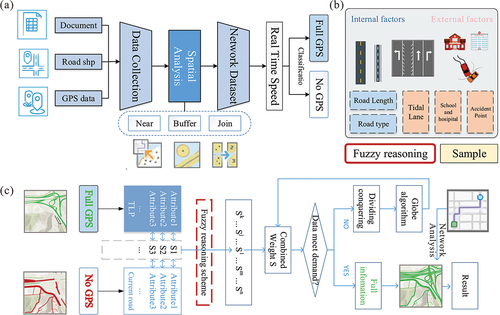
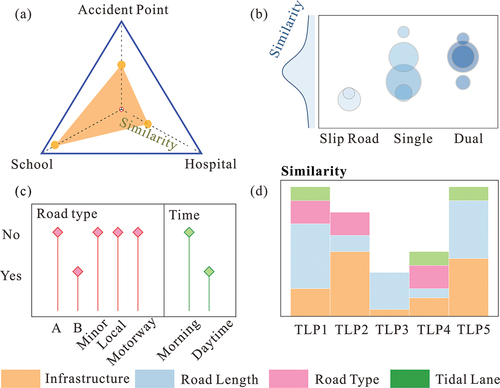
In this section, we introduce the methodology of this study. The flowchart of the proposed methodology has been illustrated in Figure 1. The core methodology includes three main aspects: selecting Typical Link Patterns (TLPs), computing the similarity degree between a road link and the TLP links, and finally, determining join weights. Firstly, the TLP is extracted considering the road characteristics (Figure 1(a,b)). Secondly, the join weights of road network are calculated (Figure 1(c)). Thirdly, a full-information road network was generated using fuzzy inference. Finally, the dividing-conquering strategy and globe algorithm are introduced.

Figure 1. The flowchart and conceptual illustration include the input data and processing (a), extract TLP considering the road characteristics (b), and the calculation of join weights (c).

2.1. Extraction typical link patterns

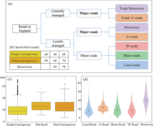
Roads have numerous properties, and we mainly consider two parts for road traffic assessments – the roads’ characteristics (road grade, road length, number of lanes, etc.) and external factors affecting traffic (weather, distance from infrastructure, tidal effect, traffic accident, etc.). For the roads’ characteristics, road type and classification determine the material of the road and its roughness, design capacity, road width, and other characteristics. This paper takes the city of Newcastle in the UK as a case study. Table 1 shows the speed limit for various types of roads in UK traffic. The data come from https://www.gov.uk/speed-limits.

Table 1. National speed limits of UK road.

Grade	Built-up areas mph (km/h)	‘A’ road mph (km/h)				Motorways mph (km/h)
Speed limit	30 (48)	40 (64)	50 (80)	60 (96)	70 (112)	60 (96)	70 (112)

For external factors, weather is one of the most important external factors affecting vehicle speed. The weather’s (we just take heavy rain and snow into consideration) impact on traffic is related to the urban Digital Elevation Model (DEM). It has the same impact on the road in a flat area and has a different impact on steep road areas and bridge sections. Furthermore, when it rains, the low places are usually impacted more seriously, and when it snows, steep road areas and bridge sections are impacted more seriously (Avila and Mezic 2020). In addition, infrastructure, such as schools, hospitals, stores, tourist resorts, and tolls, also impacts traffic, and the impacts have significant temporal characteristics. The accident point also has an important impact on traffic, which may be related to the characteristics of the road itself. Near the accident point, vehicle speed may be high (Hall and Madsen 2022).

According to the road attributes and speed limits provided by the UK’s Department for Transport, the roads in the UK are divided into centrally managed and locally managed roads, as shown in Figure 2(a). Centrally managed major roads including Trunk Motorways and Trunk A roads. Locally managed roads include all classifications of roads. The speed limit of each grade road is shown in Figure 2(b). Through the above roads’ characteristics and external factors, a representative number of typical road sections can be extracted from road links as a template, and we call this template TLP. We used the following criteria to select appropriate TLP: (a) These TLPs have full information, which means that both average speeds and the factors impacting traffic on these road links are known; (b) The extraction of TLP must consider covering all attributes and must be representative; (c) The selected TLP considers various road types and classifications in Figure 2. According to the statistics on the vehicle speed of the road sections, the speed distribution of each road section is different, as shown in Figure 2(c,d). The selected TLP category is the Cartesian product of three types (Single Carriageway, Slip Road, and Dual Carriageway) and five road classifications (A Road, B Road, Local Road, Minor Road, and Motorway).

Figure 2. Classification and types of roads in England (a), road speed limits stipulated by the Department for Transport (b), and GPS speed distribution of different classifications (c) and types (d) of roads. The colors of the boxplot correspond to the road speed limit colors (b), and the violin plot colors correspond to the classification of UK roads (a).

2.2. Road network weight calculation

Road network topology is represented in the geospatial field by a polyline, and similarity can be obtained by comparing the attribute values to TLPs. In the network, the weight of each link is determined based on the similarity of TLPs. Similarity degrees between the link and all TLP links form an n-dimensional vector (called a similarity vector). The TLPs’ weight represent road speed and it was extracted using our criteria (see Section 2.1). The similarity vector was conferred by comparing the attributes field between the link and TLPs, then the weight of the link was calculated.

The environmental factors in this paper include road types and classifications, link length, tidal factors, distance from infrastructure, and accident points, representing the link geospatial structure distribution. We reckon the weight of the link according to the similarity degree with the TLPs:

(1) $\begin{array}{c}Lin{k}_i=\frac{{\sum }_{k=1}^n{S}_i^{k}Lin{k}^k}{{\sum }_{k=1}^n{S}_i^k}\end{array}$(1)

where the total number of TLPs is n, Link^k is the corresponding weight of the typical pattern link k (k ∈ 1…n), similarity degree $S_i^k$ is the geographic fuzzy membership value of the link i to typical pattern link k, and Link_i is the weight of link i.

Similarity degree is the index to measure two variables’ similar relationship. Before getting similarity between link i (Link_i) and TLP t (TLP_t, t = 1…n), we need to calculate the set of environmental factors relative to TLP_t, which will be formed as a vector of similarity degree. Suppose there are m TLPs and n attributes involved in the calculation. The similarity S^v in the properties between the road P being reasoned and typical road $T_t\left(t\in \left[1\dots m\right]\right)$ is calculated as follows:

(2) $\begin{array}{c}\left\{\begin{array}{c}{S}_{i,t}^v=e^{{\left(\frac{\left|p_i^v-p_t^v\right|}{w_1}\right)}^{2}ln\left(k_1\right)}{p}_i^v<p_t^v\\ S_{i,t}^v=1p_i^v=p_t^v\\ S_{i,t}^v=e^{{\left(\frac{\left|p_i^v-p_t^v\right|}{w_2}\right)}^{2}ln\left(k_2\right)}{p}_i^v>p_t^v\end{array}\right.\end{array}$(2)

where $S_{i,t}^v$ is the similarity between the current path and the i-th attribute corresponding to a typical road TLP_t, $p_i^v$ is the i-th value of the current road attributes, and $p_t^v$ is the value of TLP_t. w₁, w₂, k₁, and k₂ are adjustment parameters, and we can divide the fuzzy membership curve into three models (bell-shaped, Z-shaped, or S-shaped, as shown in Figure 3) by adjusting these four parameters. When $w1=w2$ and $k1=k2\ne 1$, it is a bell-shaped curve. When $k1=1$ and $k2\ne 1$, it is a Z-shaped curve. When $k2=1$ and $k1\ne 1$, it is a S-shaped curve. In the S-shaped or Z-shaped curve, the value of k1 is usually set at 0.5.

Figure 3. Similarity curve: Bell-shaped (a), S-shaped (b) and Z-shaped (c).

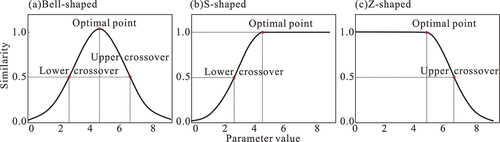
A bell-shaped curve suggests that the similarity degree is high when the parameter is close to the critical value. Conversely, the similarity degree is low when the parameter is far from the critical threshold; the Z-shaped curve reflects that the parameter value is lower and that the similarity degree is higher. The similarity gradually decreases when the value becomes greater than the critical threshold; however, the S-shaped curve expresses that the similarity degree reaches its maximum when the environmental factor value is greater or equal to the critical threshold. These three types of similarity curves and critical values are determined by actual situations. In this study and in most cases, a bell-curve is used. There will be a low level of similarity if the value exceeds or below the threshold too much.

2.3. Fuzzy inference

TLP has unique characteristics (i.e. road types and classifications, link length, and other properties). We can calculate link environmental factors using Geographic Information Science (GIS) geospatial technology, then compare the link attributes with those TLP values and acquire the similarity degree of the multi-dimensional vector. Figure 4 shows a schematic illustration and similarity calculation based on TLP.

Figure 4. Conceptual illustration of similarity calculation. Left column shows a 5-dimensional similarity vector illustration. The right column shows examples of similarity and speed calculations.

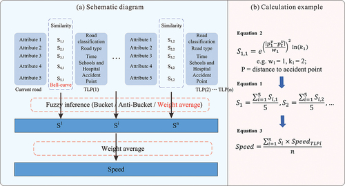
The key to fuzzy inference is to calculate the joint weight, which is done by measuring the similarity between the link and TLP under each influencing factor. It can be explained through a conceptual illustration (Figure 5). Figure 5(a) shows the similarity of attributes space considering infrastructure and the accident point factor. The external vertices of the triangle represent one TLP strict value of the distance from infrastructure (for example, 500 m is considered a threshold), and the internal shadow of the triangle illustrates similarity degree compared with the TLP. Figure 5(b) shows the degree of road classification’s similarity between links and TLP. Figure 5(c) directly judges the type and period of the road through the values of Yes and No. The similarity of the n-dimensional vector for all TLPs represents the link to its comprehensive characteristics, as shown in Figure 5(d).

Figure 5. Conceptual illustration of attributes similarity between link and TLP. First, calculate the similarity of attributes space considering infrastructure and accident point factor (a). Then calculate the road classification’s similarity between links and TLP (b), judging the type and period of the road through the values of yes and no (c). Finally, the n-dimensional vector’s similarity is acquired for all TLPs, representing the link and its comprehensive characteristics.

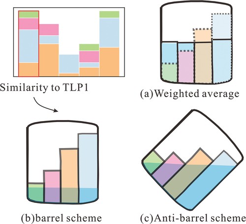
It needs fuzzy inference to determine the TLP link type. There are maximum and minimum values in the similarity vector. The maximum value means that the link attribute is the most conducive factor to turn into the TLP, and the minimum value indicates that the link attribute is the biggest obstacle to becoming the type of TLP. Three strategies were proposed to make a decision, barrel scheme, anti-barrel scheme, and weighted average scheme.

The barrel scheme says the barrel’s capacity is not determined by the longest wooden bars but by the shortest. The barrel method suggests taking the minimum value in the vector as the similarity degree for one TLP and then taking the maximum from all similarity degree values to determine the link ownership of TLP, as shown in Figure 6(b). The anti-barrel scheme is the opposite of the barrel method. The longest piece of wood establishes the barrel’s characteristics and personality, which better represents the link’s unique features. This method recommends taking the maximum value in the vector as the similarity degree for one TLP and then taking the maximum from all similarity degree values to determine the link ownership of TLP, as shown in Figure 6(c). The weighted average scheme is the middle of the barrel scheme and anti-barrel scheme. It takes the weighted average of values in the vector as the similarity degree for one TLP, and then from all similarity degree values, and it takes the maximum to determine the link ownership of TLP, as shown in Figure 6(a). This paper uses a weighted average scheme.

Figure 6. Conceptual illustration of barrel theory, anti-barrel theory and weighted average.

2.4. Algorithm design for fuzzy inference

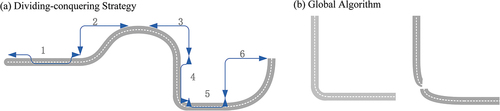
Fuzzy inference is used to judge membership between the link and TLP. The next step is to calculate the weight value, and two algorithms are considered – the Dividing-Conquering Strategy (DCS) and Globe Algorithm (GA).

DCS assumes that any complex thing could be divided into simple sub-components. Therefore, a large complex problem can be decomposed into small, simple problems. Then the small problems are solved using the recursion method, and the solution set of small problems constitutes the solution to the big problem. DCS divides the entire twisting and turning road into some sub-links. It is worth noting that the sub-link has a typical single characteristic. Figure 7(a) sketches the whole link and the sub-links. Calculate each sub-link similarity to TLP and obtain sub-link weight by the linear weighted method. The whole link weight can be calculated by accumulating the weights of sub-links, as in the following equation:

Figure 7. The whole link is divided into sub-links (a) and sub-links into whole link (b).

(3) $\begin{array}{c}{\mathrm{W}}_x=\sum _{i=1}^n\left(Le{n}_i\times \sum _{j=1}^m\frac{S_{ij}\times W_j}{S_{ij}}\right)\end{array}$(3)

W_x is the weight of link x to be observed, n is the number of sub-links, Len_i is the distance of sub-link i, m is the number of types of TLP, S_ij is similarity of sub-link i to TLP j, and W_j is the weight of TLP j.

GA does not break the whole link into sub-links. The accumulation summation of local links could not reflect the actual situation, and it ignores the whole link integrity and uniqueness in a particular spatial location. When using DCS, the whole link is divided into two sub-links in a particular location. Take the corner of a link as an example. The environmental factors of each sub-link connection area are likely to be ignored in their special features as the integrated part of the link. In other words, the uniqueness is turning flat and smooth. Figure 7(b) shows that the whole link itself holds a bending feature, but the two sub-links contain straight line characteristics after being decomposed, which may lead to local errors. GA compares the whole link to the TLP to obtain the similarity degree, and the parameter is used for making some adjustments, as in the following formula:

(4) $\begin{array}{c}\left\{\begin{array}{c}{W}_x=Le{n}_x\times \sum _{j=1}^m\frac{S_j\times W_j}{S_j}\times p\\ p=1W_j<1\\ p=\sum _{i=1}^n\left(1+\frac{Attri{b}_i-Opti{m}_i^{\ast }}{Opti{m}_i}\right)W_j=1\end{array}\right.\end{array}$(4)

where Len_x is length of the whole link x, m is the number of types of TLP, S_j is the similarity to TLP_j, W_j is the weight of TLP_j, parameter p is the factor of adjustment, n is the number of environmental factors of TLP, Attrib_i is the attribute of the link, and Optim_i* is the TLP value of attribute i. Parameter p is used when the link attribute is larger than the limit value of TLP (distance value is far from TLP critical threshold, above 5% e.g.), which is needed to adjust the weight of the link.

DCS and GA reveal the membership between the link and TLP from different perspectives. DCS focuses on the accuracy of each sub-link weight, but it ignores the integrated uniqueness at the limited geospatial location. Meanwhile, GA takes the link as the whole one, and it smoothens the whole link. It can be applied to the situation that the length of the road links is long, and the speed of the vehicles at the start and end of these links can be ignored; however, the precision of GA is poorer than DCS in smoothing geospatial places. Application of the algorithm should be based on the environment reality background to pick the appropriate method.

3. Materials

3.1. Study area

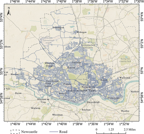
The area this paper chose to study is Newcastle (Figure 8), which is located between 1°46′ W – 1°32′ W and 54°67′ N – 55°04′ N. There are three reasons why Newcastle were used as the case study area: (a) The transportation network in Newcastle has obvious temporal and spatial characteristics, particularly with higher traffic volume and congestion during the morning peak hour in the city center; (b) Newcastle has various road types and classifications, all the road of each type are marked in road network shapefile; and (c) high-frequency GPS and substantial statistical data can be obtained from the British Road Bureau, so it is an ideal area for the study.

Figure 8. Map of the road network (blue line) distribution in Newcastle, the dotted line represents the border of Newcastle.

3.2. Data

The data used in this paper include road network data, GPS data, infrastructure data, road traffic information, and traffic accident records. The extraction of data is shown in Table 2.

Table 2. Data used in this work.

Data	Format	Source	Data extraction
Road network	shapefile	OpenStreetMap(OSM)	The line shapefile is extract by Newcastle boundary
GPS data	shapefile	Ordnance Survey, OSM, and Department for Transport	The average vehicle speed for different time periods on each road was extracted from GPS data
Vehicle speed	table	Department for Transport	Each road’s average speed was calculated
Hospital	XY coordinates	OSM	Integrating XY coordinates into vector point data
School	XY coordinates	Google Earth	Integrating XY coordinates into vector point data
Accident	table	Department for Transport	The accident point was extracted when accident severity reached a fatal level

The road network data came from OpenStreetMap (OSM) (https://www.openstreetmap.org/). The road vector map was obtained through OSM, and then the network dataset was constructed. At the same time, OSM provided some GPS data, but not complete data. More GPS data were extracted from the Department for Transport and Ordnance Survey Mastermap Highways Network (https://www.ordnancesurvey.co.uk/business-government/products/mastermap-highways-speed-data). Table 3 shows a sample of GPS data, and with the average vehicle speed of for different time period.

Table 3. Data used in this work.

class	index	ID	length	speed	time	formOfWay
A Road	1	A188	49.517	17.958	M	Single Carriageway
Local Road	3		68.507	2.556	M	Single Carriageway
…	…	…	…	…	…	…

The Department for Transport of the UK (https://www.gov.uk/government/organisations/driver-and-vehicle-standards-agency/) provides road information, including speed limit information on different roads, road speed conditions at different times, and road categories. The hospital data come from OSM Medical and the schools come from the coordinate system provided by Google Earth. The accident point data comes from the UK government’s Open Data website, published by the Department for Transport. The UK government collects and publishes (usually annually) detailed information on road accidents across the country. This information includes geographic location, weather conditions, vehicle types, casualties, and vehicle maneuvering, making it a very interesting and comprehensive dataset for analysis and research (https://data.gov.uk/). The accident point in this study was selected when accident severity reached a fatal level.

4. Empirical application

4.1. Road network speed features

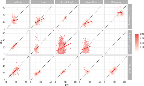
Classify Newcastle’s entire road network into two categories: complete information and incomplete information, and the time is the morning peak period. Each category randomly selects the same number of links as TLP (observed) and the predicted links. Figure 9 shows the observed versus predicted average link speeds distribution by road type and classification. This figure is a scatterplot, where the red line represents the linear regression fit. The proposed method shows robustness at the more disaggregate level to which this method is calibrated (i.e. by road type and classification). During the morning rush hour, the average speed of various road observations is 19.478 mph, and the average speed of the fuzzy inference is 18.719 mph, with a deviation of 3.89%. Predictions and observations are highly consistent in most classifications and types, especially for A road, B road, dual carriageway, and slip road. Notably, this method captures the peaks of the distribution, especially for single carriageway.

Figure 9. Scatterplots between observed GPS speed (y-axis) and fuzzy inference predicted average link road speed (x-axis). The red line represents the linear regression fit.

4.2. Road network time features

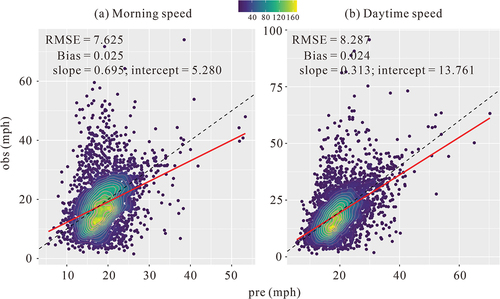
Newcastle’s entire road network can be classified into two categories – complete information and incomplete information – and all periods are selected. Each category randomly selects the same number of links as TLP (observed) and predicted links. Figure 10 shows the distribution of observed versus predicted average link speeds during the morning peak and the daytime. The speed of the morning rush hour on various types and classifications of roads is significantly lower than that of the daytime. The average observed speed in the morning peak is 19.478 mph, and the average observed speed in the daytime is 21.541 mph; the average predicted speed in the morning peak is 18.719 mph, and the average observed speed in the daytime is 20.702 mph. There is reasonable temporal variation in Newcastle speeds. In addition, the high speed of vehicles during the day is higher than that of the morning rush hour.

Figure 10. Observed GPS speed (y-axis) and fuzzy inference predicted average link road speed (x-axis) scatterplots in morning (a) and daytime periods.

4.3. Fuzzy inference method cross-validation

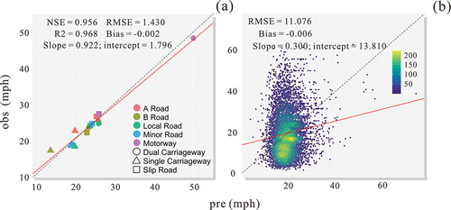
Then switching to the cross-validation (Figure 11), calculate the average speed for each road type and classification (Figure 11(a)). The model’s statistical metrics show high robustness. The NSE and R square values are 0.956 and 0.968, respectively. The results in the cross-validation suggest that our method is robust across a wide range of road types and classifications with different time periods. Figure 11(b) shows a comparison of observed versus predicted for all road link speeds. The figure’s yellow color scheme and legend highlight the number of data points (density) of the validation data set.

Figure 11. Cross-validation results. First, calculate the average speed for each road type and classification (a), then compare observed versus predicted for all road link speeds (b).

4.4. Fuzzy inference road network path planning

This paper applies the fuzzy inference to Newcastle. The road network in Newcastle has certain characteristics, and the transport network has obvious temporal and spatial characteristics. The traffic congestion phenomenon is obvious in the morning rush period. This paper used the classical A* algorithm to test the optimal path planning between two points with the static and fuzzy impedance models, respectively. To ensure the fairness of the results, the test took the same start time and from/to place. Two experiments were conducted for various routes in the study area during the morning peak and daytime. The routes had different starting and ending points. A total of 13,987 samples were selected for typical road sections. The sample selections considered different road characteristics. Table 4 shows the sample selection process.

Table 4. Sample selection categories and data statistics.

Road Type	Road Classification	Time	Distance to infrastructure	Distance to accidental point	Sample number
A road	Single Carriageway	Morning	<100 m	<100 m	5
	Dual Carriageway	Morning	100–300 m	>300 m	35
	Slip Road	Morning	>300 m	>300 m	272
	Slip Road	Daytime	>300 m	100–300 m	103
B road	Single Carriageway	Morning	100–300 m	<100 m	6
	Dual Carriageway	Daytime	>300 m	>300 m	109
	Slip Road	Daytime	100–300 m	<100 m	1
Local Road	Single Carriageway	Morning	<100 m	>300 m	76
	Slip Road	Morning	>300 m	>300 m	1503
	Dual Carriageway	Daytime	>300 m	<300 m	2
Minor Road	Single Carriageway	Morning	<100 m	100–300 m	15
	Dual Carriageway	Morning	>300 m	>300 m	10
Motorway	Dual Carriageway	Daytime	>300 m	>300 m	8
	Slip Road	Daytime	>300 m	>300 m	1

A total of two tests were carried out for the study area. First, three groups were tested to study the practical application of fuzzy inference when the road information is incomplete. The first group of tests seeks to select different periods and carry out comparative experiments using traditional static impedance, that is, using the road length as the default impedance for the path planning (Figure 12(a)), and dynamic impedance, that is, estimating incomplete road network information based on GPS real-time data. The data were then divided into daytime (Figure 12(b)) and morning peak (Figure 12(c)). The routing results were summarized from the length of the planned route, the length of the high-grade road in the planned route, and the estimated travel time. The results are shown in Table 5. Through fuzzy impedance, although the total length of the road slightly increased, the proportion of fast-moving roads is higher, and the estimated arrival time is shorter.

Figure 12. The results of the first group of tests select different time periods and carry out comparative experiments. Static (a) and fuzzy impedance models (b-c) routing results comparison in daytime and morning.

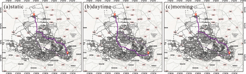
Table 5. Comparison of statistical indexes on static and fuzzy impedance models.

algorithm	Route length (km)	High-grade road crossed (km)	Evaluated travel time(min)
Static impedance	14.850	30.968	28.772
Fuzzy daytime	15.513	34.714	26.812
Fuzzy morning	14.878	31.411	28.419

The second group of tests select daytime periods and carry out comparative experiments using traditional static impedance, that is, using the road length as the default impedance for path planning (Figure 13(a1,b1)), and dynamic impedance, that is, estimating incomplete road network information based on GPS real-time data (Figure 13(a2,b2)). The routing results are summarized from the length of the planned route, the length of the high-grade road in the planned route, the estimated travel time, and the number of schools and hospitals passed by. The results are shown in Table 6. Through the fuzzy impedance, although the total length of the road slightly increased, the proportion of fast-moving roads is higher. The roads prone to congestion, such as schools and hospitals, were avoided. It is more aligned with driving habits, and the estimated arrival time is shorter. This means that the impedance model based on fuzzy inference has a practical application.

Figure 13. The results of the second group of tests select daytime periods and carry out comparative experiments. Static (a1, b1) and fuzzy impedance models (a2, b2) routing the results comparison in the daytime.

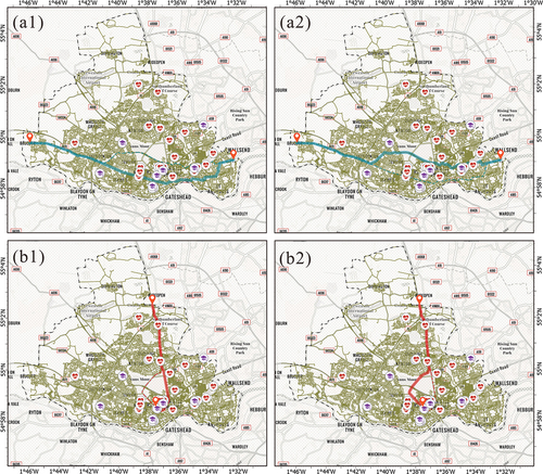
Table 6. Comparison of statistical indexes on static and fuzzy impedance models.

Algorithm	Route length (km)	High-grade road crossed (km)	Evaluated travel time(min)	Infrastructure number
Static impedance	16.418	32.186	30.606	4
Fuzzy impedance	16.425	36.420	27.059	1

5. Discussion

This paper generates data covering the entire road network based on incomplete GPS road information. The road speed was estimated based on the third law of geography, considering the similarity between data-missing road sections and TLP. The reliability and robustness of the method in this paper were proved by the driving speed prediction results of each road’s classification and type. In similar studies, due to the consideration of geographical similarity and the use of global algorithms and divide-and-conquer strategies, the estimation accuracy is better than that of support vector machines (Mohandes et al. 2004), and the complexity is less than that of fuzzy neural networks (Tang et al. 2017). By considering the driving time and environment, road congestion is avoided during the morning rush hour, which is more reasonable than the static impedance results in the absence of GPS data.

This paper chose Newcastle as the research area. The selection of road characteristics is different in different research areas, and the estimation results will also differ. The traffic impact factors analysis and their quantification are the keys of this method. Whole and detailed factors can improve the accuracy of routing. The relationship between the factors and traffic is also very important. This paper brings out three kinds of relationships, and it requires more simulation experiments to describe the relationship if users require more accurate results.

The roads in each city are different, and the factors that impact traffic are also different. The strategy of computing weights depends on the attributes of the road. Therefore, factors in more typical cities may be analyzed and tested, and it can enrich this method further. For example, in mountainous areas with large terrain fluctuations, the influence of DEM must be considered (especially on rainy and snowy days) or in areas with many traffic accidents, where the vehicle speed at the points where traffic accidents are prone to occur is relatively high. More factors should be selected and applied to practical research, and the method in this paper can be extended to more areas.

6. Conclusions

Road links with full information are the basis of routing. Looking at the situations where GPS data cannot cover the whole road link. This paper proposes a fuzzy inference method to assign weights for road networks based on incomplete information. The TLPs are extracted first according to these related factors. The environmental factors in this paper include road types and classifications, link length, tidal factors, distance from infrastructure, and accident points. The core methodology road link and the TLPs, and finally, determining join weights. Taking the Newcastle traffic information as an example, the cross-verification results show robustness: The average RMSE is 1.430 mph, and the bias is 0.2%; the overall RMSE is 11.067 mph, and the bias is 0.6%. The route planning result of fuzzy inference is faster, avoids roads prone to congestion. The expected arrival time was shorter, and the average travel time was reduced by 6.5%. In future studies, it is recommended to analyze and test a broader range of representative cities and incorporate additional features. Moreover, the method proposed in this paper then should be dynamically adjusted in specific regions, making our results more accurate and applicable.

Disclosure statement

No potential conflict of interest was reported by the author(s).

Data availability statement

Data will be made available on request.

Additional information

Funding

This work was supported by the National Key Research and Development Program of China [grant number 2019YFC1804304], the National Natural Science Foundation of China [grant number 41771478], and the Fundamental Research Funds for the Central Universities [grant number 2019B02514].

Notes on contributors

Longhao Wang

Longhao Wang received the B.S. degree from Hohai University, Nanjing, China, in 2022. He is currently pursuing the Ph.D. degree in the Key Laboratory of Water Cycle and Related Land Surface Processes, Institute of Geographic Sciences and Natural Resources Research, Chinese Academy of Sciences, Beijing, China. His research interests include geo-information processing, remote sensing hydrology and application.

Xiaoping Rui

Xiaoping Rui received his PhD degree from the Institute of Remote Sensing Applications, Chinese Academy of Sciences, Beijing, China, in 2004. He is currently a professor with the School of Earth Sciences and Engineering, Hohai University, Nanjing, China. His research interests include traffic optimization and resource allocation, remote sensing applications and deep learning.

References

- Akhtar, M., S. Moridpour, and M. Bazant. 2021. “A Review of Traffic Congestion Prediction Using Artificial Intelligence.” Journal of Advanced Transportation 2021:1–18. https://doi.org/10.1155/2021/8878011.
- Avila, A. M., and I. Mezic. 2020. “Data-Driven Analysis and Forecasting of Highway Traffic Dynamics.” Nature Communications 11 (1): 2090. https://doi.org/10.1038/s41467-020-15582-5.
- Calabrese, F., M. Colonna, P. Lovisolo, D. Parata, and C. Ratti. 2011. “Real-Time Urban Monitoring Using Cell Phones: A Case Study in Rome.” IEEE Transactions on Intelligent Transportation Systems 12 (1): 141–151. https://doi.org/10.1109/TITS.2010.2074196.
- Castro, P. S., D. Q. Zhang, C. Chen, S. J. Li, and G. Pan. 2013. “From Taxi GPS Traces to Social and Community Dynamics: A Survey.” ACM Computing Surveys 46 (2): 1–34. https://doi.org/10.1145/2543581.2543584.
- Chen, P., R. Tong, B. Yu, and Y. P. Wang. 2020. “Reliable Shortest Path Finding in Stochastic Time-Dependent Road Network with Spatial-Temporal Link Correlations: A Case Study from Beijing.” Expert Systems with Applications 147:113192. https://doi.org/10.1016/j.eswa.2020.113192.
- Deng, S. J., S. Y. Jia, and J. Chen. 2019. “Exploring Spatial-Temporal Relations via Deep Convolutional Neural Networks for Traffic Flow Prediction with Incomplete Data.” Applied Soft Computing 78:712–721. https://doi.org/10.1016/j.asoc.2018.09.040.
- Guo, Y., B. Li, Z. Lu, and J. Zhou. 2022. “A Novel Method for Road Network Mining from Floating Car Data.” Geo-Spatial Information Science 25 (2): 197–211. https://doi.org/10.1080/10095020.2021.2003165.
- Hall, J. D., and J. M. Madsen. 2022. “Can Behavioral Interventions Be Too Salient? Evidence from Traffic Safety Messages.” Science 376 (6591): 370. https://doi.org/10.1126/science.abm3427.
- Huang, B., Q. Wu, and F. B. Zhan. 2007. “A Shortest Path Algorithm with Novel Heuristics for Dynamic Transportation Networks.” International Journal of Geographical Information Science 21 (6): 625–644. https://doi.org/10.1080/13658810601079759.
- Huo, J., X. H. Wu, C. Lyu, W. B. Zhang, and Z. Y. Liu. 2022. “Quantify the Road Link Performance and Capacity Using Deep Learning Models.” IEEE Transactions on Intelligent Transportation Systems 23 (10): 18581–18591. https://doi.org/10.1109/TITS.2022.3153397.
- Karamete, B. K., L. Adhami, and E. Glaser. 2021. “An Adaptive Markov Chain Algorithm Applied Over Map-Matching of Vehicle Trip GPS Data.” Geo-Spatial Information Science 24 (3): 484–497. https://doi.org/10.1080/10095020.2020.1866956.
- Li, B., Z. S. Xu, and Y. X. Zhang. 2021. “Two-Stage Multi-Sided Matching Dispatching Models Based on Improved BPR Function with Probabilistic Linguistic Term Sets.” International Journal of Machine Learning and Cybernetics 12 (1): 151–169. https://doi.org/10.1007/s13042-020-01162-y.
- Li, X., W. Shu, M. Li, H. Huang, P. Luo, and M. Wu. 2009. “Performance Evaluation of Vehicle-Based Mobile Sensor Networks for Traffic Monitoring.” IEEE Transactions on Vehicular Technology 58 (4): 1647–1653. https://doi.org/10.1109/TVT.2008.2005775.
- Lu, J., B. Li, H. Li, and A. Al-Barakani. 2021. “Expansion of City Scale, Traffic Modes, Traffic Congestion, and Air Pollution.” Cities 108:102974. https://doi.org/10.1016/j.cities.2020.102974.
- Mi, J., Y. L. Bai, M. B. Luo, H. Wang, and M. R. Chen. 2019. “Microscopic Estimation of Road Impedance by Decomposing Traffic Delay into Individual Road Segments: An Analytical Approach.” Mathematical Problems in Engineering 2019. https://doi.org/10.1155/2019/3285498.
- Minguez, R., S. Sanchez-Cambronero, E. Castillo, and P. Jimenez. 2010. “Optimal Traffic Plate Scanning Location for OD Trip Matrix and Route Estimation in Road Networks.” Transportation Research Part B-Methodological 44 (2): 282–298. https://doi.org/10.1016/j.trb.2009.07.008.
- Mohandes, M. A., T. O. Halawani, S. Rehman, and A. A. Hussain. 2004. “Support Vector Machines for Wind Speed Prediction.” Renewable Energy 29 (6): 939–947. https://doi.org/10.1016/j.renene.2003.11.009.
- Munizaga, M. A., and C. Palma. 2012. “Estimation of a Disaggregate Multimodal Public Transport Origin-Destination Matrix from Passive Smartcard Data from Santiago, Chile.” Transportation Research Part C-Emerging Technologies 24:9–18. https://doi.org/10.1016/j.trc.2012.01.007.
- Neuhold, R., and M. Fellendorf. 2014. “Volume Delay Functions Based on Stochastic Capacity.” Transportation Research Record 2421 (1): 93–102. https://doi.org/10.3141/2421-11.
- Olayode, I. O., L. K. Tartibu, and M. O. Okwu. 2021. “Prediction and Modeling of Traffic Flow of Human-Driven Vehicles at a Signalized Road Intersection Using Artificial Neural Network Model: A South African Road Transportation System Scenario.” Transportation Engineering 6:100095. https://doi.org/10.1016/j.treng.2021.100095.
- Shang, P., R. Li, J. Guo, K. Xian, and X. Zhou. 2019. “Integrating Lagrangian and Eulerian Observations for Passenger Flow State Estimation in an Urban Rail Transit Network: A Space-Time-State Hyper Network-Based Assignment Approach.” Transportation Research Part B-Methodological 121:135–167. https://doi.org/10.1016/j.trb.2018.12.015.
- Sun, S., C. Zhang, and G. Yu. 2006. “A Bayesian Network Approach to Traffic Flow Forecasting.” IEEE Transactions on Intelligent Transportation Systems 7 (1): 124–132. https://doi.org/10.1109/TITS.2006.869623.
- Tang, J., F. Liu, Y. Zou, W. Zhang, and Y. Wang. 2017. “An Improved Fuzzy Neural Network for Traffic Speed Prediction Considering Periodic Characteristic.” IEEE Transactions on Intelligent Transportation Systems 18 (9): 2340–2350. https://doi.org/10.1109/TITS.2016.2643005.
- Wang, C. X., S. Zourlidou, J. Golze, and M. Sester. 2021. “Trajectory Analysis at Intersections for Traffic Rule Identification.” Geo-Spatial Information Science 24 (1): 75–84. https://doi.org/10.1080/10095020.2020.1843374.
- Wang, L. H., J. Wu, R. Li, Y. J. Song, J. Y. Zhou, X. P. Rui, and H. W. Xu. 2021. “A Weight Assignment Algorithm for Incomplete Traffic Information Road Based on Fuzzy Random Forest Method.” Symmetry-Basel 13 (9): 1588. https://doi.org/10.3390/sym13091588.
- Wong, W., and S. C. Wong. 2016. “Network Topological Effects on the Macroscopic Bureau of Public Roads Function.” Transportmetrica A: Transport Science 12 (3): 272–296. https://doi.org/10.1080/23249935.2015.1129650.
- Xu, Y. Y., L. E. Olmos, S. Abbar, and M. C. Gonzalez. 2020. “Deconstructing Laws of Accessibility and Facility Distribution in Cities.” Science Advances 6 (37). https://doi.org/10.1126/sciadv.abb4112.
- Yang, B., M. Kaul, and C. S. Jensen. 2014. “Using Incomplete Information for Complete Weight Annotation of Road Networks.” IEEE Transactions on Knowledge and Data Engineering 26 (5): 1267–1279. https://doi.org/10.1109/TKDE.2013.89.
- Yang, H. 1995. “Heuristic Algorithms for the Bilevel Origin Destination Matrix Estimation Problem.” Transportation Research Part B-Methodological 29 (4): 231–242. https://doi.org/10.1016/0191-2615(95)00003-V.
- Yao, Y., Z. Peng, and B. Xiao. 2018. “Parallel Hyper-Heuristic Algorithm for Multi-Objective Route Planning in a Smart City.” IEEE Transactions on Vehicular Technology 67 (11): 10307–10318. https://doi.org/10.1109/TVT.2018.2868942.
- Ye, Q., W. Y. Szeto, and S. C. Wong. 2012. “Short-Term Traffic Speed Forecasting Based on Data Recorded at Irregular Intervals.” IEEE Transactions on Intelligent Transportation Systems 13 (4): 1727–1737. https://doi.org/10.1109/TITS.2012.2203122.
- Yu, Y., K. Han, and W. Ochieng. 2020. “Day-To-Day Dynamic Traffic Assignment with Imperfect Information, Bounded Rationality and Information Sharing.” Transportation Research Part C-Emerging Technologies 114:59–83. https://doi.org/10.1016/j.trc.2020.02.004.
- Zhang, T., W. Zhang, and Z. He. 2021. “Measuring Positive Public Transit Accessibility Using Big Transit Data.” Geo-Spatial Information Science 24 (4): 722–741. https://doi.org/10.1080/10095020.2021.1993754.
- Zhu, A. X., G. Lu, J. Liu, C. Z. Qin, and C. Zhou. 2018. “Spatial Prediction Based on Third Law of Geography.” Annals of GIS 24 (4): 225–240. https://doi.org/10.1080/19475683.2018.1534890.