Chart features, data quality, and scale in cartographic sounding selection from composite bathymetric data

ABSTRACT

Cartographic sounding selection is a constraint-based bathymetric generalization process for identifying navigationally relevant soundings for nautical chart display. Electronic Navigational Charts (ENCs) are the premier maritime navigation medium and are produced according to international standards and distributed around the world. Cartographic generalization for ENCs is a major bottleneck in the chart creation and update process, where high volumes of data collected from constantly changing seafloor topographies require tedious examination. Moreover, these data are provided by multiple sources from various collection platforms at different levels of quality, further complicating the generalization process. Therefore, in this work, a comprehensive sounding selection algorithm is presented that focuses on safe navigation, leveraging both the Digital Surface Model (DSM) of multi-source bathymetry and the cartographic portrayal of the ENC. A taxonomy and hierarchy of soundings found on ENCs are defined and methods to identify these soundings are employed. Furthermore, the significant impact of depth contour generalization on sounding selection distribution is explored. Incorporating additional ENC bathymetric features (rocks, wrecks, and obstructions) affecting sounding distribution, calculating metrics from current chart products, and introducing procedures to correct cartographic constraint violations ensures a shoal-bias and mariner-readable output. This results in a selection that is near navigationally ready and complementary to the specific waterways of the area, contributing to the complete automation of the ENC creation and update process for safer maritime navigation.

KEYWORDS:

• Bathymetry
• generalization
• cartography
• hydrography
• navigation
• nautical
• automation
• Electronic Navigational Charts (ENC)

1. Introduction

Changes in seafloor topography are constantly being measured, charted, and disseminated by hydrographic organizations and cartographic production entities around the world. The primary medium for visualizing the seafloor for maritime navigation purposes is the Electronic Navigational Chart (ENC), whose usage is mandatory on Safety Of Life At Sea (SOLAS) regulated vessels. ENCs are vector-based digital nautical charts consisting of attributed (IHO 2014) point, polyline, and polygon objects that represent essential navigational information, e.g. soundings, depth contours, dredged channels, rocks, wrecks, obstructions, etc. ENC data are visualized for the mariner through an on-board Electronic Chart Display and Information System (ECDIS), which references the internationally standardized attributes to symbolize features (IHO 2017a, 2017c).

As new data reflecting changes in seafloor topography are collected, ENCs are updated to reflect this information. New ENCs can also be generated for uncharted regions or when data coverage areas change (Nyberg et al. 2020). Due to the volume of incoming data and resultant time and cost burden associated with managing entire suites of ENCs, automating components of the cartographic generalization process is crucial to maintaining ENC integrity and increasing throughput. Following a natural disaster, for example, accurate and consistent cartographic generalization algorithms can be employed to efficiently update ENCs for safe navigation. Similarly, these same methods could be utilized to generate ENCs for a newly charted location.

Industries adjacent to the nautical charting community, such as hydrography, are also streamlining data management, collection, and distribution. Methods for processing bathymetric measurements are being extensively researched (Calder and Mayer 2003; Šiljeg et al. 2022; Stateczny et al. 2021). Increased data are becoming available as surveying navigationally significant near-shore areas becomes more economically viable (Szafarczyk and Toś 2022), which are being used in wider seabed analyses (Janowski et al. 2022).

The National Bathymetric Source (NBS) project of the National Oceanic and Atmospheric Administration’s (NOAA) Office of the Coast Survey (OCS) are developing a comprehensive bathymetric database to support nautical charting in U.S. waters (Rice et al. 2020). The database will consist of the best quality data available and their associated metadata to provide a multi-source, multi-platform, high-resolution, seamless composite bathymetric layer. Combined with methods in automated nautical cartography, such as the algorithm proposed in this work, bathymetric features of ENCs can be derived for any location where NBS data is available, thus significantly decreasing the time-burden associated with the creation or maintenance of ENCs.

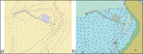
ENCs have an optimal viewing scale for their navigational purpose (Weintrit 2018), at which incoming source data must be cartographically generalized. This generalization process is often performed in a multi-scale database environment, where the conceptual framework is a hybrid (Stoter et al. 2010) of the version proposed by Brassel and Weibel (1988), which separates Digital Landscape Models (DLMs) and Digital Cartographic Models (DCMs). Data composing the ENCs are stored at lower resolutions, which have been cartographically generalized for visualization at the optimal viewing scale. The DCM is generated via the ECDIS using pre-determined portrayal rules (IHO 2017a). An example of the difference between the DLM in the cartographic database using default portrayal in a GIS environment versus the corresponding DCM on the ECDIS screen is illustrated in Figure 1.

Figure 1. Geographic objects (a) versus cartographic portrayal (b) for ENC US5DE1EGM.

Cartographers utilize various generalization operators (see Roth, Brewer, and Stryker 2011) for different types of features found on ENCs. Spot depths (soundings), for example, are generalized to the scale of a target chart by eliminating (also referred to as omission) less important soundings according to nautical cartographic constraints. Depth contours are generalized using geometric operators such as simplification, smoothing, aggregation, and exaggeration. Thus, generalization in nautical cartography is a difficult and nuanced challenge, where methods must be tailored for specific feature types and bound by strict constraints to promote safe navigation.

Sounding selection is a major generalization task and bottleneck in the ENC creation/update process, as it requires a tedious examination of soundings from high-resolution bathymetry data. Methods for automating this task have been published in the literature; however, these algorithms have limitations that can lead to critical cartographic constraint violations and undermine safe maritime navigation: operating strictly in the DLM-space and disregarding cartographic portrayal, which is what mariners use to navigate; not validating navigational safety; focusing on less navigationally relevant cartographic constraints; excluding existing ENC features into the selection process that affect sounding distribution; and overlooking bathymetric data quality.

In this work, a comprehensive sounding selection algorithm is applied to composite bathymetric datasets to contribute to an automated ENC-ready selection. This is achieved by testing the algorithm against NBS bathymetry data, analyzing characteristics of both the Digital Surface Model (DSM) of the bathymetry and DCM of the ENC, defining a hierarchy of sounding type and importance, identifying all soundings through the lens of safe navigation, utilizing additional bathymetric features and ENC characteristics to achieve a complimentary sounding distribution, and incorporating correction procedures for cartographic constraint violations to ensure a shoal-bias selection.

The remainder of this paper is organized in the following manner: Section 2 introduces cartographic sounding selection, Section 3 discusses related work, Section 4 proposes the new methodology, Section 5 presents experimental results, Section 6 provides concluding remarks, and the Appendix provides additional tables.

2. Background

Sounding selection can be separated into two categories: hydrographic and cartographic. Hydrographic sounding selection is the process of generalizing bathymetry data to produce a shoal-biased, less dense, and more manageable subset of soundings to facilitate the subsequent cartographic selection (Dyer, Kastrisios, and De Floriani 2022; MacDonald 1984; Oraas 1975; Zoraster and Bayer 1992). Cartographic sounding selection is the identification of soundings for chart display. The cartographic selection limits the quantity of soundings to the least amount necessary to illustrate the seafloor while maintaining readability when other seafloor features are present, such as depth contours, rocks, wrecks, and obstructions. Cartographic sounding selection also requires a taxonomy and hierarchy of sounding type and importance, relative to safety. The distribution of the cartographic selection is typically concentrated in regions that are challenging to navigate, i.e. shallow waters and locations with submerged topographic features, and less dense in other areas, such as deep waters and relatively flat seafloor.

There are various methods in the literature to derive the cartographic selection directly from high-resolution source bathymetry; however, these approaches do not assess the cartographic representation of the selected soundings or existing ENC features and thus, can select sounding distributions that would make the ENC illegible when rendered at scale for the mariner. At present, cartographic sounding selection remains a semi-manual process (Kastrisios and Calder 2018). The reader is referred to Dyer et al. (2022), which provides a detailed discussion of the cartographic representation of ENC soundings.

The generalization of data for an ENC, including bathymetry, must adhere to constraints for safe maritime navigation. Adapted from Ruas and Plazanet (1997) and Zhang and Guilbert (2011), these constraints within the context of sounding selection are defined as follows:

1. Functionality: emphasize features relevant to the purpose of the chart, which is safe navigation. This is often referred to as the safety constraint, or shoal-bias, where depth information on the chart must not appear deeper than the source data.

2. Legibility: the perceptibility threshold of features on a chart. It is necessary to assess the DCM of the chart as well as human feature separation and visibility limits (see Rytz et al. 1980) to detect legibility issues.

3. Displacement: the maximum allowed displacement of an object according to its nature. The point of origin for a sounding label must not be displaced from the source data; however, depth contours may be displaced in favor of safety to navigation.

4. Shape: although the level of detail is reduced during generalization, characteristics and the general shape of the seafloor should be preserved. Morphological details should be maintained as much as possible.

There is a hierarchy among these constraints, which must be respected when balancing the inherent trade-offs between each constraint. Functionality is the most critical for safe navigation and highest priority for every feature on the ENC, which must not be violated. The equilibrium between adhering to the remaining constraints is unique for each feature type. The legibility and displacement constraints are equally as important for sounding labels, where labels must be readable and exact locations of depths must be preserved. The readability of individual sounding labels conflicts with the morphology constraint, where high-density sounding distributions result in better descriptions of the seafloor, albeit at the expense of overlapping sounding labels (Dyer, Kastrisios, and De Floriani 2022). Nevertheless, if shallow depths are preserved, eliminating soundings in favor of legibility over morphology is acceptable where overlapping labels are indistinguishable from each other, regardless of seafloor topographic complexity. Moreover, constraints of one feature type can influence constraint adherence for another type. When a depth contour overlaps a sounding label, for example, the contour may be displaced around the label to maintain readability, but the sounding cannot be displaced. On the other hand, overlaps between depth contours and soundings are easier to distinguish than two overlapping sounding labels (Kastrisios et al. 2023). Therefore, there is not only a hierarchy for cartographic constraints, but also for feature types, which demonstrates the complementary nature between features such as soundings and depth contours and why additional ENC features are required during sounding selection as well as the complexity of the problem.

Cartographic principles to help guide the highly involved sounding selection process have been established by the International Hydrographic Organization (IHO) (2017c). These principles are as follows:

1. Maximum and minimum depths for an area of the chart should always be shown. This includes least depths over shoals, banks, or bars in navigable channels as well as lines of deepest depths for navigation in narrow passageways.

2. The selected soundings and depth contours should complement each other in representing the seafloor characteristics. Steep gradients should be represented by contours to avoid over-plotting distortions with soundings.

3. The density of soundings should be determined by the seafloor topography. Flat or evenly sloped areas should show minimal, evenly spaced soundings where the distance between soundings increases with depth. Conversely, irregular seafloor topography should be represented by a denser and most likely irregularly distributed sets of soundings.

These guidelines form a hierarchy of sounding importance and when combined with charting practices of the Office of Coast Survey (OCS) (NOAA 2021), five distinct types of soundings can be identified on ENCs, listed below in descending order of importance:

1. Least Depth: the shallowest sounding of a seafloor feature, e.g. the pinnacle of a seamount, dome, or ridge, that is delineated by a closed depth contour. Least depth soundings should always be portrayed even if their depth is equal to the depth contour.

2. Shoal: the shallowest local sounding representing the depth over an isolated shoal, which may or may not be delineated by a depth contour. A least depth sounding is always a shoal sounding, but a shoal is not always a least depth sounding; the location (inside or outside of a closed depth contour) is the determining factor.

3. Deep: the deepest local sounding, e.g. a depression and/or potential transportation route. If chart space is limited, shallower soundings shall take precedence over deep soundings.

4. Supportive: soundings that portray additional information to the mariner about the seafloor morphology. These soundings are often utilized to illustrate changes in bottom slope away from least depth, shoal, and deep soundings.

5. Fill: soundings to estimate depths between widely spaced depth contours and portray a smooth seafloor.

Least depth soundings are the highest priority and must always be retained as they represent the shallowest depths in the bathymetry and “peaks” in the seafloor topography. The quantity and distribution of least depth soundings are directly related to the depth contours of the bathymetry, where they are only found inside the shallowest closed depth contours. Depth contours are often displaced during generalization to emphasize safety and/or sounding label legibility. An isolated cluster of shallow peaks, for example, may be aggregated within a single depth contour if appropriate for the scale. This in turn would affect the quantity and distribution of least depths, where only the shallowest peak inside the depth contour would be identified as a least depth sounding (see Section 4.2). Although ranked with higher precedence, it is noted that least depth soundings are a sub-category of shoal soundings. Least depth soundings are shoal soundings with the condition that they are the shallowest shoal sounding inside a shallow closed depth contour, i.e. if the shallowest contour is two meters the contour must be two meters (Figure 2(b), showing shoal versus least depth). Shoal soundings can be found both inside and outside of depth contours.

Figure 2. Taxonomy of soundings present in an ENC from differing perspectives: (a) cross-section and (b) two-dimensional ENC view.

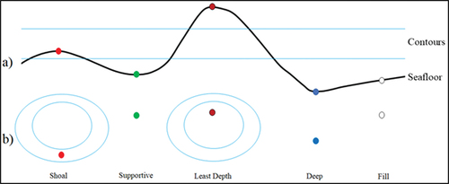
Shoal, deep, and supportive soundings indicate unexpected local depths and changes in seafloor slope. The primary purpose of a shoal sounding is to indicate a shallow depth located in relatively deeper water. Opposite of least depth and shoal soundings are deep soundings, which represent “pits” in the seafloor topography. Deep soundings help identify routes across a waterway for larger draft vessels. Supportive soundings are often found near least depth, shoal, and deep soundings, and indicate to the mariner a changing seafloor topography. Together, shoal, deep, and supportive soundings tend to be irregularly distributed and concentrated in areas of high relief.

Least depth, shoal, deep, and supportive soundings correspond to the critical points of a bathymetric surface model, where least depth and shoal soundings are local maxima, deep soundings are local minima, and supportive soundings are saddle points of the modeled seafloor. Therefore, topological characteristics of the bathymetric surface model must be analyzed to identify these sounding types. Similar approaches have been used for spot height identification in topographic mapping (Rocca, Jenny, and Puppo 2017).

Fill soundings, also referred to as background soundings, are the lowest in the hierarchy, most versatile, and utilized in varying capacities. Traditionally, the selection of fill soundings has followed a triangular or rhomboidal distribution to create an aesthetically pleasing result. A significant portion of the literature is focused on fill sounding selection and more contemporary methods focus on leveraging fill soundings to satisfy the morphology constraint (Li et al. 2021; Yu 2018). Regardless, satisfying the functionality and legibility constraints should be the primary goal when selecting soundings through the lens of safe navigation.

Figure 2 shows an example of the sounding taxonomy described above, where Figure 2(a) shows a cross-section perspective and Figure 2(b) shows the same soundings shown from the two-dimensional ENC perspective.

3. Related work

The generalization paradigms and methods by which the taxonomy of soundings is utilized during cartographic sounding selection vary across the literature. Current approaches disregard the cartographic representation of features, which can lead to legibility constraint violations and render an ENC unreadable. Current methods also do not assess cartographic constraint adherence or bathymetric data quality during selection. Moreover, soundings are often selected based on less navigationally relevant constraints (morphology) and only incorporate depth contours into the selection process (if at all), while other features can also affect sounding distribution.

Zoraster and Bayer (1992) determined the importance of each sounding by assessing how closely the depth of a sounding can be estimated by interpolating between depth contours. Once a sounding is selected, an area buffer (increasing size with depth) around that sounding is calculated, following Oraas (1975), to remove any soundings inside the buffer from consideration. While they did not consider a hierarchy or taxonomy of soundings, they were the first to use chart features (depth contours) and incorporate components of hydrographic sounding selection into to the cartographic selection process.

Tsoulos and Stefanakis (1997) constructed a Triangulated Irregular Network (TIN) from the input soundings and adjacent triangles within the same depth range are then merged into polygons, which are subsequently assessed for the shallowest soundings. An equilateral triangular grid is overlaid, and fill soundings are identified by matching soundings to the grid nodes. This method is the first to delineate different types of soundings and perform a sequential approach to selection.

Sui et al. (1999) built on the radius-based method of Oraas (1975) where the soundings are first generalized using a variable-size buffer increasing with depth and depth contours are extracted from a TIN derived from the remaining generalized soundings. A point-in-polygon algorithm is used to ensure each area between depth contours contains a sounding. This work was continued by Sui et al. (2005), where known navigational hazards were incorporated by separating soundings that fall within navigational hazard areas and generalizing these soundings based on the average slope of soundings in the area. These were the first works to incorporate the morphology constraint (slope) directly into the generalization algorithm.

Du et al. (2001) and Jingsheng and Yi (2005) defined a theoretical model based on clustering and seafloor topography. Sounding clusters are identified based on depth and location, which are then triangulated and identified as sub-areas. The clusters are formed based on depth ranges, where adjacent sub-groups covering the same depth range are merged. A tree-based data structure is then used to identify shoal, deep, and fill soundings, where the nodes of the tree are sub-groups, edges are the relationships of sub-groups, and the root of the tree is the shallowest value. Sub-groups are identified as ridges, sea-route, or topographically complex and generalized accordingly. The idea of generalizing based on seafloor classification types was further developed by Lovrinčević (2019), who also incorporated metrics of slope, maximum horizontal distance, and a four-meter deviation from surrounding depths to select soundings. The selection was performed by identifying soundings located on different topographic features, i.e. depression, ridge, basin, etc.

Yu (2018) combined clustering methods and the morphology constraint to generalize fill soundings based on point density and uses a measure of bathymetric complexity. Polygons are generated for each sounding cluster and the bathymetric complexity for each polygon is evaluated using a composite index. Additional fill soundings are retained in areas of higher seafloor complexity compared to lower complexity.

Li et al. (2021) also focused on the morphology constraint, where the bathymetry is generalized using a function to preserve seafloor topography. Shoal and deep soundings are first identified from the Digital Elevation Model (DEM) through a neighborhood comparison method and the DEM is used for describing seafloor topography. The remaining soundings are assigned an importance value using an inverse distance-weighted function, where soundings with larger values better describe seafloor topography. The final selection is achieved by sorting all soundings from shallow to deep and selecting soundings with higher importance when they have the same depth.

Skopeliti et al. (2020) proposed a method to select soundings from a DEM, using a taxonomy of sounding types and a grid superimposed over the original bathymetry. Soundings are selected for each grid cell based on the sounding hierarchy. The shallowest sounding for each grid cell is selected as well as the deepest sounding where the depth difference is greater than 20%. The shallowest and deepest soundings are then selected for each remaining empty grid cell, and fill soundings are selected using a minimum distance metric. Lastly, the selection of soundings per grid cell is modified to maintain a minimum distance between them.

Spot-height identification is a similar task in topographic mapping where elevation data are generalized to determine relative peaks in elevation. Baella et al. (2007) and Palomar‐Vázquez and Pardo‐Pascual (2008) first categorized elevations of interest and then classified these elevations based on geomorphometric characteristics, which then drove the generalization. Chaudhry and Mackaness (2008) proposed a method to delineate between mountain ranges and the individual hills of which they are composed. Rocca et al. (2017) determine the lifespan of DEM critical points in a continuous scale-space model to determine the importance of feature elevations. Arundel and Sinha (2020) utilize a two-part procedure to incrementally move lower elevations uphill and to reference higher resolution data. While spot-height elevation and sounding selection are similar in theory, the cartographic constraints and use-cases of final products are not comparable and should not be conflated.

The primary limitation of the existing methods for sounding selection is that the functionality constraint is not evaluated despite the existence of well-defined tests. Furthermore, variable size buffers or grids are used to try to avoid sounding label overplot; however, none of the existing methods assess or the DCM to avoid legibility issues, which is what the mariner uses to navigate. Additionally, as Dyer et al. (2022) showed, user-defined radius- and grid-based techniques often result in functionality constraint violations. Another issue arises with existing chart features not considered for the sounding selection, such as wrecks, rocks, obstructions, etc., where these features can overplot with soundings and reduce readability. Lastly, methods focusing on the morphology constraint do not follow the hierarchy to the cartographic constraints and largely ignore legibility in favor of morphology which can lead to violations of the functionality and legibility constraints (Dyer, Kastrisios, and De Floriani 2022).

Existing approaches also do not leverage any metrics of uncertainty during selection, which is intrinsic to modern bathymetry data processing (see Calder and Mayer 2003). Moreover, these approaches assume the input bathymetry is single-sourced and data quality is homogenous. This is increasingly not the case, where composite datasets are being compiled from multiple sources to create a seamless layer, such as the NBS effort.

Therefore, in this work, a comprehensive sounding selection algorithm is introduced for use with composite bathymetric data focused on safe navigation. Adherence to the defined cartographic constraints are quantitatively assessed and corrected for in the final selection, toward an ENC-ready selection.

4. Proposed methodology

The work of Dyer et al. (2022) is built upon to leverage the cartographic portrayal of the ENC and propose a cartographic sounding selection process guided by the defined cartographic constraints. Moreover, existing ENC features and corrections of cartographic constraint violations are included for the selection. The proposed algorithm also follows internationally established cartographic rules aiming to support safe navigation (IHO 2017c), which leads to the following sequential workflow:

1. Critical point identification

2. Depth contour generalization and least depth sounding selection

3. Generalization leveraging the cartographic representation of features

4. Shoal, deep, and supportive sounding selection

5. Fill sounding selection

6. Assessment and correction of cartographic constraint violations

Figure 3 illustrates the workflow where inputs and outputs are parallelograms and processes are rectangles.

Figure 3. Workflow diagram of proposed methodology.

4.1 Critical point identification

As described in Section 2, the critical points of a bathymetric surface model correspond to least depth, shoal, supportive, and deep soundings. Moreover, soundings surrounding the input bathymetry as well as existing ENC bathymetric features that affect sounding distribution must also be examined during cartographic sounding selection.

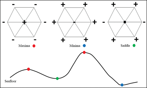
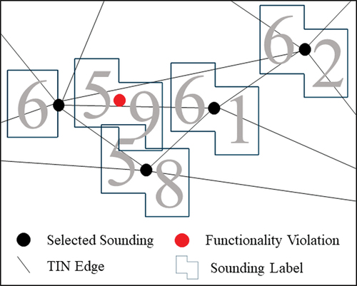
Critical points are identified by assessing the connectivity information associated with the vertex-to-vertex relationships of points in a TIN surface model (Banchoff 1970). Figure 4 illustrates the vertex relationships of critical points on a TIN and their distribution on the seafloor. In comparison to Figure 2(a), it is clear how the critical points of a bathymetric DSM correspond to least depth, shoal, deep, and supportive soundings.

Figure 4. Vertex to vertex relationships of the critical points of a bathymetric surface model and their distribution on the seafloor.

When the bathymetric surface model is constructed for critical point extraction, the convex hull of the input point set will be generated, and if regions of the domain are concave, edges can connect points that should not be connected. For example, bathymetry is often collected in areas near islands, jetties, and breakwaters where soundings on either side of the object are not real-world neighbors. Similarly, dredged areas (DRGARE in S-57 (IHO, 2014)) are representative polygons illustrating areas maintained to a specific depth, known as the controlling depth, which are used on ENCs instead of soundings. Therefore, when constructing the bathymetric surface model, the triangulation is constrained to exclude dredged areas and land areas (areas above the 0-meter contour) to prevent the creation of soundings across land areas and maintained channels.

Existing chart soundings (or bathymetry data) surrounding the survey area must also be included in the bathymetric surface model to identify critical points along the boundary of the survey area, where without vertex connectivity information, critical points could not be identified. Additionally, rocks, wrecks, and obstructions can carry depth information, representing peaks in the seafloor (local maxima), which can affect critical point distribution.

The survey soundings, surrounding soundings, rocks, wrecks, and obstructions are combined into a single point set. A convex hull polygon is generated for these features, serving as the ENC coverage area. Overlapping regions of the ENC coverage polygon and dredged area polygons are eliminated from the ENC coverage polygon. The resulting ENC coverage polygon is then converted to polylines, where vertices along the 0-meter depth contours are assigned depths of zero and vertices along the dredged areas are assigned the controlling depth value. The combined point set is triangulated and constrained to the ENC coverage polyline boundary. Each node of the triangulation is visited, and nodes identified as critical points are flagged as a maxima, minima, or saddle point.

4.2 Depth contour generalization and least depth sounding identification

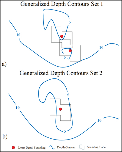
Algorithmically, least depth soundings are relatively simple to calculate: a point-in-polygon operation is performed using a closed depth contour and the shallowest sounding inside the polygon is selected. Conversely, depth contour generation is more challenging than it may seem. Specifically, contours must not violate the functionality constraint by portraying the seafloor as deeper than the real world, i.e. contours must always be generalized toward deeper water. Furthermore, depending how depth contours are generalized, the contour geometry can affect least depth sounding quantity and distribution. This is shown in Figure 5, where two sets of generalized contours result in different quantities least depth soundings.

Figure 5. Least depth sounding selection from two sets of generalized depth contours.

The proposed approach accepts depth contours as input to be utilized during the selection process. There are two paradigms in nautical cartography to achieve generalized shoal-bias depth contours appropriate for a given scale. The first approach involves generalizing the bathymetry with shoal-bias and extracting the depth contours from the generalized surface (Peters, Ledoux, and Meijers 2014). This method provides an intrinsic form of feature simplification and aggregation and can achieve aesthetically pleasing contours; however, it is difficult to determine the seaward displacement of the contours from smoothing. Moreover, if a dataset contains measurement above and below the waterline, the 0-meter contour will be displaced and shallow soundings could appear to be on land. The second method requires first extracting the depth contours and then generalizing their geometry (Guilbert 2016; Guilbert and Lin 2006; Guilbert and Saux 2008; Li et al. 2018; Skopeliti et al. 2021; Smith 2003). These methods may be more automated in nature but can result in topological inconsistencies in the resultant output, such as self-intersection or crossing geometries. Consequently, there is not a single accepted solution across the field.

The depth contour generalization method adopted for this work is that proposed by Peters et al. (2014), which has been implemented by Environmental Systems Research Institute (ESRI) (ArcPro version 3.0), where a TIN is generated from a set of soundings and iteratively smoothed with shoal-bias using a set number of user-defined iterations and contours extracted (ESRI 2022).

The process for extracting the least depth soundings consists of converting the shallowest closed depth contours to polygons and using a point-in-polygon algorithm to identify the shallowest sounding inside the polygon. If the least depth is a rock, wreck, or obstruction, a sounding is not selected. Least depth soundings are selected without assessing their cartographic representations at scale, which can cause legibility issues between these soundings. This is primarily attributable to depth contours that have not been appropriately generalized for the target scale (Figure 5). Thus, legibility issues between least depth soundings can indicate further generalization of the depth contours is required and can be flagged for the cartographer.

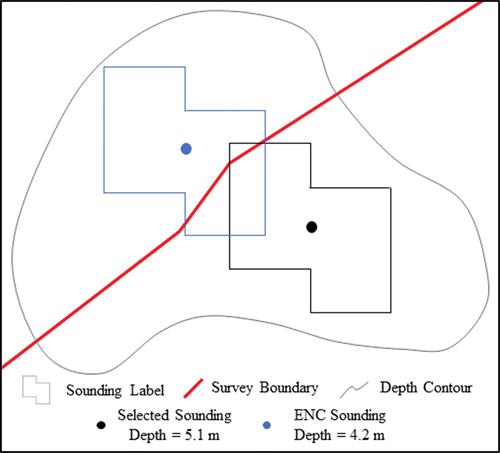
Legibility issues with least depth soundings can also occur with soundings surrounding the boundary of the survey. When legibility violations such as these occur (Figure 6), the least depth is only selected if it is shallower than the ENC sounding.

Figure 6. Example of legibility violation between selected sounding and surrounding ENC sounding, where the ENC sounding is shallower than the selected sounding.

This approach to least depth sounding selection satisfies the first and second cartographic guidelines recommended by the IHO. The selected least depth soundings are added to a list, named preliminary selection, which stores the currently selected soundings.

4.3 Generalization leveraging the cartographic representation of features

The work by Dyer et al. (2022) provided a means to avoid legibility issues between individual soundings. Following the same logic, functionality and legibility issues with existing ENC features such as rocks, wrecks, and obstructions should be avoided as well. Moreover, soundings outside the survey boundary must be included to reduce legibility violations between the selected soundings for the survey and those outside the extent. By including soundings outside the survey extent, deeper soundings inside the survey are removed from potential selection which would have been otherwise selected (Figure 6). Therefore, the approach by Dyer et al. (2022) is extended to include existing ENC features and soundings surrounding the survey extent to eliminate these issues. These features are identified from the extent of the survey area and the feature symbol is calculated to IHO standards (IHO 2017c).

Dyer et al. (2022) followed a sequential approach for sounding label generalization to first remove deep soundings directly inside the shallow sounding label footprint and then remove deep soundings that overlap the shallow label. The algorithm presented in this work performs only a single pass on the input soundings, eliminating soundings inside the footprint and overlaps simultaneously. Performing a single pass increases performance but can result in additional functionality violations. However, a cartographic constraint violation correction procedure is introduced that removes any remaining functionality constraint violations from the final selection.

The input consists of the flagged survey soundings described in Section 4.1 (surface critical points), surrounding soundings outside the survey extent, existing ENC features (rock, wreck, and obstructions) and scale at which the data is to be generalized. The soundings are inserted into a bucketed point-region (PR) quadtree (Samet 1984), where sounding indices are stored in its leaf nodes. The cartographic representations of the existing ENC features are then used to traverse the quadtree and remove any overlapping soundings. An auxiliary list is created containing the indices of the remaining survey and surrounding soundings sorted from shallow to deep. Beginning with the first element in the soundings list, the sounding label footprint is calculated, which is then used to traverse the quadtree and indices of deeper soundings overlapping the label footprint are removed from the quadtree and auxiliary list. This results in a sounding set that exhibits no legibility issues with individual soundings or dangerous seafloor features.

4.4 Shoal, deep, and supportive sounding selection

As described in Section 2 and Section 4.1, shoal, deep, and supportive soundings correspond to the critical points of a bathymetric surface model. Moreover, legibility violations between features must be avoided. Therefore, these soundings are selected from the subset derived in the previous section, where sounding labels do not overplot with each other or dangerous seafloor features. Soundings flagged as “maxima” are selected as shoals; soundings flagged as “minima” are selected as deeps; and soundings flagged as “saddle” are selected as supportive.

Due to the difference of selecting least depth soundings from the un-generalized bathymetry, and selecting shoal, deep, and supportive soundings from the generalized soundings, legibility issues can arise. Therefore, shoal, deep, and supportive soundings are only selected if there are no legibility violations with any least depth sounding. The shoal, deep, and supportive soundings are combined into a list and sorted from shallow to deep. Beginning with the shallowest sounding, soundings are inserted into preliminary selection, which is currently composed only of least depth soundings, if no legibility violations are present. This is then repeated for the remaining soundings.

The proposed method for shoal, deep, and supportive sounding selection satisfies the first and third cartographic guidelines for sounding selection recommended by the IHO. Maximum and minimum depths are selected, and the sounding distribution is based on the underlying bathymetric surface model, where selected soundings are concentrated in regions with increased seafloor complexity.

4.5 Fill sounding selection

Traditionally, fill soundings have been selected to simply fill gaps between least depth, shoal, deep, and supportive soundings. This usually followed aesthetic-based criteria and allowed the mariner to interpolate depths between widely spaced contours. Data-driven approaches can also effectively select fill soundings, particularly with respect to the morphology constraint. However, functionality and legibility should be favored over the morphology constraint, and fill soundings are selected through the lens of safe navigation and chart readability. Two different types of fill soundings are selected to achieve a balance between aesthetics and data-driven approaches.

Fill soundings using a variable length radius-based approach (Oraas 1975) are identified first to select soundings based on depth, ensuring the third IHO cartographic guideline for sounding selection. Remaining fill soundings are selected based on the surface test (Kastrisios et al. 2019a), which leverages bathymetric data quality to identify fill soundings in areas where the real-world depth significantly deviates from the expected value.

4.5.1 Variable length radius selection

The variable length radius-based generalization method consists of sorting a list of soundings from shallow to deep, applying a buffer to the shallowest sounding in the list, and removing deeper soundings inside the buffer from the list. The buffer radius is increased in length for the next sounding, and the process is repeated for the remaining soundings in the list until all soundings have been examined.

The length of the buffer radius is subjective (fixed or variable), and in contrast to existing methods that propose specific values (Oraas 1975; Skopeliti et al. 2020; Sui et al. 1999; Sui, Zhu, and Zhang 2005; Tsoulos and Stefanakis 1997; Zoraster and Bayer 1992), the starting and ending radii lengths are determined in this work from the soundings present in ENCs in the local area at the same scale. This accounts for the fact that there are not universal values for every waterway and geographic configurations of each ENC can vary, which require different distributions of soundings. Utilizing this existing chart information, a fill sounding distribution complementary to the waterway is achieved. Figure 7 shows an example of the radius-based generalization applied to different waterway types, which illustrates there are not universal parameters and should optimally be calculated based on the ENC geography.

Figure 7. Radius-based generalization applied to different waterways.

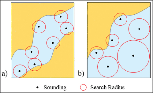
Figure 7(a) shows a narrow waterway, such as a river or channel, where shallow depths are located near the shoreline (retained) and deeper depths are near the center of the channel (eliminated). Figure 7(b) shows an open-water region where depths increase with distance from the shoreline. When soundings in Figure 7(b) are generalized using the same length radius as in Figure 7(a), both shallow and deep soundings are retained. Deeper soundings have longer radii lengths, as the radius length increases with depth. Thus, the distribution of the bathymetric survey extent and geography of the charted area can affect fill sounding distribution. Utilizing the ENC sounding distribution as input for the variable length radius generalization ensures an output consistent with the waterway.

The variable length radius-based generalization method is applied to the generalized output derived in Section 4.3. The distance between nearest neighbor soundings is calculated for each sounding in the ENC of interest. Distances between soundings corresponding to the minimum and maximum depths found in the input bathymetry are used for starting and ending radius lengths, respectively. The radius-fill soundings are then sorted from shallow to deep and inserted into preliminary selection only if no legibility violations with least depth soundings are introduced.

4.5.2 Surface test selection

Following the aesthetic-based fill sounding selection, a data-driven approach is utilized, the surface test, that incorporates a global uncertainty measurement of the bathymetric survey, called Category Zones of Confidence (CATZOC), to identify soundings that significantly deviate from the expected depth.

CATZOC, as defined by the IHO, is an indication that a particular survey meets minimum criteria for position and depth accuracy based on specific standards (IHO 2017b). This information is encoded in an ENC as a polygon object representing an area associated with a specific CATZOC value. Surveys are assigned a CATZOC value of A1, A2, B, C, D, or U in descending order of accuracy, which indicates a global measure of position and depth uncertainty at the 95% confidence interval. Uncertainty is a function of depth that increases with depth. Table 1 summarizes the standards of the IHO for assessing the CATZOC value of a survey.

Table 1. Summary of the depth and uncertainty criteria for CATZOC Assessment.

CATZOC	Position Uncertainty	Depth Uncertainty	Example Depth	Example Depth Uncertainty
A1	±5 meters + 5% of depth	.5 + 1% of depth	10 m	±.6 m
A2	±20 m	1 + 2% of depth	10 m	±1.2 m
B	±50 m	1 + 2% of depth	10 m	±1.2 m
C	±500 m	2 + 5% of depth	10 m	±2.5 m
D	Worse than C	Worse than C	N/A	N/A
U	Unassessed	Unassessed	N/A	N/A

The depth contours derived using the methods described in Section 4.2 are combined with any rocks, wrecks, or obstructions, as well as the soundings of preliminary selection, then converted to a TIN using a constrained triangulation to enforce contour edges. Next, for each triangle of the TIN, the soundings composing the triangle vertices are assessed. Composite bathymetry datasets can contain soundings with varying CATZOC values; therefore, the strictest CATZOC value is determined from the triangle vertices. The soundings derived from generalizing using cartographic representations (Section 4.2) that intersect the triangle are then determined to be within the expected depth uncertainty (Column 3, Table 1) tolerance based on the CATZOC value. The expected depth value of each sounding intersecting the triangle is interpolated using the barycentric coordinates of the sounding and the depth values of the soundings forming the triangle (Figure 8). This expected depth value is compared to the actual depth of the sounding and if the difference is greater than the depth uncertainty tolerance for the given CATZOC and depth, the sounding is added to preliminary selection, as long as there are no legibility issues with least depth soundings. After each triangle has been assessed, the contour vertices and updated preliminary selection are re-triangulated and the process is repeated until none of the triangles contain soundings outside the depth tolerance.

Figure 8. Surface test fill sounding selection procedure.

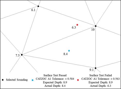
As shown in Table 1, survey soundings with CATZOC D or U do not have a quantified depth uncertainty range, and therefore, no tolerance with which to compare the expected and interpolated depths. As such, the implemented approach is to skip the triangle if the vertices are completely composed of these types of soundings, which can be modified to user needs by setting a depth tolerance.

4.6 Assessment and correction of cartographic constraint violations

Methods for assessing the adherence of a sounding selection to the constraints of nautical cartography have been published in the literature (Dyer, Kastrisios, and De Floriani 2022) and are utilized in this work, where functionality violations are determined using the triangle test, legibility violations are identified by locating over-plotting sounding labels and existing chart features, displacement is violated when a sounding is repositioned from its original location, and morphology is determined by examining seafloor roughness before and after generalization. The adherence of preliminary selection to the cartographic constraints is evaluated and corrective procedures are applied to eliminate functionality violations while minimizing legibility violations.

The first corrective procedure minimizes legibility violations between depth contours and sounding labels, following the second IHO cartographic guideline. Each sounding in preliminary selection that is not a least depth is evaluated to determine if the sounding label overplots a depth contour. If there is an intersection, and the sounding depth is deeper than the value of the contour, the sounding is removed from preliminary selection. Additionally, due to the displacement of contours, deeper soundings can exist within shallow contours, i.e. a 5.1 m depth inside a 5 m contour. Retaining these soundings is not a functionality violation; however, these deep soundings are removed as they do not provide navigationally important information.

The next step iteratively corrects sounding legibility violation and functionality violations. The surrounding ENC soundings are first combined with preliminary selection to ensure there are no violations along the boundary of the bathymetric survey, and the triangle test is assessed to identify functionality violations. The generalization method using the cartographic representation of features described in Section 4.3 is then applied to the soundings (excluding least depths) to remove overplot between soundings. Next, the functionality violations are inserted into preliminary selection if no legibility violations are introduced. The functionality test is then repeated, and the process is reiterated. However, there are certain exceptions where the sounding distribution will not allow a functionality violation to be inserted without causing a legibility issue. Figure 9 illustrates this, where the violation with a depth of 5.9 cannot be corrected without introducing a legibility violation with the 5.8 sounding. These exceptions are corrected by inserting the violation after a user-defined number of iterations despite if it causes a legibility violation.

Figure 9. Exception with functionality constraint violations where legibility issues cannot be avoided.

Throughout the selection process, the introduction of legibility violations between soundings has been limited by only inserting soundings that do not over-plot with the least depth soundings. Legibility violations can still occur between individual least depth soundings and the functionality correction procedure described above can potentially introduce legibility violations. Therefore, the minimum number of legibility violations in the final selection is the number of legibility violations associated with the least depth soundings, assuming no issues are introduced during the correction. This issue can be improved or eliminated by adjusting depth contour geometries. As a result of these correction procedures, a final cartographic sounding selection with zero functionality constraint violations and a minimal number of legibility violations is achieved.

5. Experimental results

Due to the complex nature of cartographic sounding selection, unavailability of existing or easily implementable public-domain software, and incorporation of various chart features in our sounding selection process, we cannot directly compare the proposed solution to those found in the literature. Therefore, the proposed algorithm is evaluated in varying geographies following the assessment criteria in Dyer et al. (2022), while also demonstrating how the generalization of depth contours, different scales, shoreline configuration, and existing chart features can affect sounding selection and distribution. This approach was implemented in Python, leveraging the Shapley library for geoprocessing operations (Gillies et al. 2007) and a Python wrapper (Rufat 2022) of the Triangle library (Shewchuk 1996) for triangulation.

Four bathymetric datasets were provided by the NBS to demonstrate the generation of cartographic sounding selections for ENCs in different realistic scenarios. These locations were identified based on current availability, high volume of traffic, differing types of waterways, presence of ENC features affecting sounding selection, and highest resolution ENC in the area. The data were provided horizontally referenced to their respective North American Datum of 1983 Universal Transverse Mercator zone and vertically referenced to mean lower low water (chart datum). Figure 10 shows the data area boundaries (outlined in red) with a current ENC base-map showing the surrounding geographies. Table 2 provides a description of the datasets.

Figure 10. Data extents for the (a) NY Harbor, (b) Galveston Bay, (c) Mobile Bay, and (d) Savannah River data.

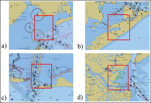
Table 2. Associated ENC information for provided bathymetric data.

Dataset Name	ENC Scale	Current NOAA ENC
New York Lower Bay, NY	1:10,000	US5NYCBG
Galveston Bay, TX	1:25,000	US5TX53M
Mobile Bay, AL	1:40,000	US5AL13M
Savannah River and Calibogue Sound, SC	1:40,000	US5GA21M

Each dataset was provided as a multi-band raster, consisting of three layers: elevation, uncertainty, and contributor, as well as an associated raster attribute table linking the contributor (source provider) information to the survey CATZOC value (see BLUETOPO (2023) for detailed specifications). The centroids of each grid cell composing the elevation band were converted to points and the associated CATZOC value for each grid cell was transferred to each point, resulting in a set of soundings consisting of values representing longitude, latitude, elevation, and CATZOC respectively.

The provided data contained interpolated depths where no hydrographic survey data was present, which was included to provide a seamless coverage area. During a real-world sounding selection process interpolated depths are omitted from potential selection. However, due to a large quantity of interpolated soundings present in the Savannah River and Galveston Bay data, these soundings were retained and assigned a CATZOC value of “U” for these datasets. This was to avoid leaving large regions of the study areas empty.

For implementing the concept of surrounding soundings explained in Section 4, a 100-meter buffer was applied to the survey area boundary and soundings within this area were used as the surrounding ENC soundings. These surrounding soundings were further generalized, resulting in a surrounding sounding set with no label overplot. The remaining soundings outside the buffer area were used as input for potential selection. This workflow was adopted to simulate the generation of sounding selections for new ENCs derived from available bathymetry; however, during the ENC update process, existing surrounding ENC soundings should be used instead.

Each of the provided datasets are near ports, where the data contain measurements above and below the water line. Measurements above the 0-meter depth contour are excluded from potential selection, as this work focuses on the bathymetric region of the ENC. This is important because how the bathymetric region of the ENC is defined can affect the number of potential soundings for selection, i.e. the displacement of the 0-meter depth contour from generalization. As previously mentioned, there is not a widely accepted solution for contour generalization and as a result, contours are accepted as input to the algorithm. To demonstrate how depth contour generalization can influence sounding selection, the results of the proposed approach using linearly interpolated (un-generalized) and generalized depth contours are compared.

The seamless data containing interpolated values were combined with rocks, wrecks, and obstructions in the area and each dataset was smoothed using iterations of 0 (linear interpolation), 500, 1000, 1500, and 2000. Results of alternative smoothing iteration values were visually inspected, and it was found that iterations below 500 did not significantly differ from linear interpolation and iterations above 2000 exceedingly displaced the contours. Contours were extracted from the smoothed surface at the depth levels defined by the IHO (2017c), i.e. 0, 2, 3, 5, 8, 10, 15, 20, 30, etc. The output of the tool consists of depth area polygons and depth contours. Minor topological inconsistencies (multi-part geometries, gaps between depth areas) in the output were manually corrected, as they would by a professional cartographer.

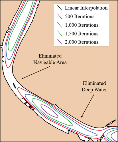
Displacement of the depth contours from generalization was highly dependent on the shoreline configuration and seafloor topography. As each of the provided datasets contained measurements above and below the waterline, iteratively smoothing the bathymetric surface displaced the 0-meter depth contour seaward, thus excluding additional soundings from potential selection, as shown in Figure 11 for the Savannah River. A small island in the middle of the narrow channel had the effect of eliminating a navigable area at higher iterations. Moreover, this region was a shallow river area with gentle to negligible slope. Thus, special consideration of the geography is required when determining the number of smoothing iterations.

Figure 11. Displacement of the 0-meter depth contour from shoal-bias smoothing of the Savannah River bathymetry.

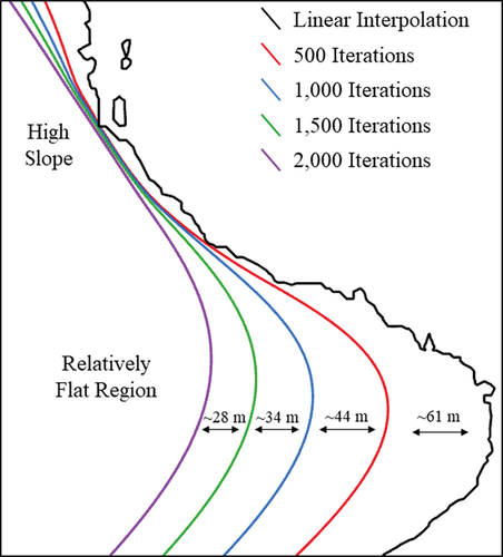
This issue is not limited to the 0-meter depth contour and can arise in relatively flat regions of the seabed, where the smoothing has a larger effect (Figure 12). The generalization of depth contours produces smooth and aesthetically pleasing results at the cost of reducing navigable waters.

Figure 12. Displacement of depth contours from smoothing in the Mobile Bay data.

The reader is referred to the Appendix for tables summarized the total quantity of soundings (Table A1) before and after filtering for interpolated values (NY Harbor and Mobile) and soundings above the waterline, and the quantity of soundings for each CATZOC value found in each filtered dataset (Table A2).

The final inputs to the cartographic selection process are the length of the radii for the radius-based fill sounding selection. These are determined from the ENCs associated with each dataset, shown in Table 2. Nearest neighbor distances between individual ENC sounding are calculated and the distances corresponding to the minimum and maximum depths found in the input bathymetry are used for starting and ending radius lengths, respectively (Table 3).

Table 3. Starting and ending radii lengths for fill sounding selection.

Dataset Name	Starting (m)	Ending (m)
New York Lower Bay, NY	34.35	230.87
Galveston Bay, TX	43.21	1117.96
Mobile Bay, AL	43.03	1309.28
Savannah River and Calibogue Sound, SC	86.69	618.12

During generalization, soundings are eliminated based on overplot with existing danger to navigation features. Generally, fewer soundings are eliminated when the number of smoothing iterations is increased, due to fewer soundings being eligible for selection from the displacement of the 0-meter depth contour. Moreover, greater numbers of soundings are eliminated at smaller scales, where symbolized features (soundings and dangers to navigation) occupy more real-world space. Table 4 summarizes the quantity of input soundings eliminated during generalization from existing features. The quantity of eliminated soundings demonstrates how influential existing features can be on sounding distribution.

Table 4. Quantity of soundings removed during generalization by existing danger to navigation features.

Dataset	Smoothing Iterations	Soundings Eliminated Due to Existing ENC Features
New York Lower Bay, NY	0	33,789
	500	33,614
	1000	33,509
	1500	24,713
	2000	33,245
Galveston Bay, TX	0	131,599
	500	114,067
	1000	107,586
	1500	102,610
	2000	97,947
Mobile Bay, AL	0	184,234
	500	180,283
	1000	178,556
	1500	177,434
	2000	176,555
Savannah River and Calibogue Sound, SC	0	61,675
	500	56,935
	1000	55,404
	1500	54,471
	2000	53,624

Table 5 summarizes the quantities of each type of sounding found in the final cartographic selections.

Table 5. Summary of sounding types found in each selection.

Dataset	Smoothing Iterations	Least Depth	Shoal	Deep	Supportive	Fill (Radius)	Fill (Surface)	Adjustment	Total
New York Lower Bay, NY	0	2221	3808	12	31	1281	330	410	8093
	500	149	4,236	11	36	1,375	449	371	6,627
	1000	121	4095	10	29	1316	352	386	6309
	1500	102	4075	11	28	1291	455	371	6333
	2000	86	4022	10	26	1272	488	381	6285
Galveston Bay, TX	0	1099	154	2	3	46	3	87	1394
	500	22	255	3	0	97	5	36	418
	1000	19	238	3	1	108	3	38	410
	1500	9	222	5	2	106	9	36	389
	2000	6	226	2	1	113	10	33	391
Mobile Bay, AL	0	1205	194	1	2	108	25	40	1575
	500	30	278	2	2	124	39	42	517
	1000	25	276	2	2	124	44	35	508
	1500	20	273	2	2	122	44	37	500
	2000	16	274	2	2	123	47	32	496
Savannah River and Calibogue Sound, SC	0	318	68	0	0	29	0	31	446
	500	23	54	0	1	50	2	28	158
	1000	18	51	1	1	54	2	22	149
	1500	16	51	0	1	55	2	15	140
	2000	17	54	1	1	52	3	14	142

Across each dataset, the quantity of least depth soundings decreased as the number of smoothing iterations increased. This is due to the aggregation of neighboring depth contours, which reduces the number of potential least depth soundings, as shown in Figure 5. This, in part, demonstrates the complementary nature between sounding selection and depth contour generalization.

The totals for shoal, deep, and supportive soundings did not follow a pattern similar to the least depths. The quantities of these soundings are related to least depth soundings, depth contour generalization, and the corrective procedures described in Section 4.6. These soundings were only selected if they did not overplot least depth soundings, which eliminated potential soundings from selection in areas concentrated with least depths. This resulted in fewer shoal soundings for outputs using linearly interpolated contours compared to those with smoothed contours. A corrective procedure was employed to eliminate deep soundings in shallow water (Section 4.6), which resulted in similar quantities of deep and supportive soundings for each output. The quantity of supportive soundings was also affected by the shoal-bias generalization of the DCM (Section 4.3). Supportive soundings are often found near shoal soundings and when the label-based generalization is applied, supportive soundings are eliminated in favor of shallower depths. This is directly related to the scale of the intended generalization, where sounding labels occupy larger real-world space at smaller scales.

The displacement of depth contours and subsequent elimination of narrow waterways from generalization also impacted the total number of soundings across each dataset, showing that the appropriate number of smoothing iterations highly depends on the waterway configuration and seafloor topography. A corrective procedure to eliminate legibility violations between depth contours and sounding labels was also employed, which also further reduced the number of all soundings that were not least depths.

The waterway configuration had a significant impact on the fill-radius soundings, where the starting and ending radius values were determined from the current ENC. The Mobile Bay and Savannah River datasets had very different starting and ending values despite being the same scale product (Tables 1 and 4). This is due to the difference in waterway types, where Mobile Bay has more open water than the Savannah River (Figure 10). Similar to other sounding types, fill-radius soundings were also only selected if there was no overplot between an existing shallow sounding.

Data quality was the determining factor for the amount of selected fill-surface soundings. Datasets composed of higher quality data (NY Harbor and Mobile Bay) exhibited significantly more fill-surface soundings. This is because higher quality data has a narrower depth uncertainty threshold (Table 1), resulting in more soundings outside the threshold and consequently selected as fill-surface soundings. Additionally, many of the soundings for the Galveston Bay and Savannah River datasets had CATZOC values of “U” (interpolated values, Table 4), which does not have a specified depth uncertainty tolerance, preventing potential selection as a fill-surface sounding.

The adjustment soundings are those introduced during the correction procedures described in Section 4.6. The quantities for each site were similar across different depth contour smoothing iterations, suggesting depth contours did not significantly affect the selection of these soundings. Generally, selections with more soundings exhibited more adjustment soundings (NY Harbor compared to Savannah River).

Finally, the total number of soundings generally decreased with additional smoothing iterations for depth contour generalization. This is primarily due to the reduced number of potential soundings for selection and movement from the 0-meter and other contours moving to deeper water. The final cartographic sounding selection totals represent an elimination of approximately 99.75% to 99.98% of the original source survey soundings. Table 6 summarizes the cartographic constraint violations for the final selections.

Table 6. Summary of cartographic constraint assessments for test datasets.

Dataset	Smoothing Iterations	Functionality	Legibility (soundings)	Legibility (dangers)	Displacement	Morphology
New York Lower Bay, NY	0	0	1886	96	0	0.08757
	500	0	95	49	0	0.08612
	1,000	0	83	47	0	0.08140
	1,500	0	75	46	0	0.08194
	2,000	0	73	45	0	0.08170
Galveston Bay, TX	0	0	1037	143	0	0.0017
	500	0	13	15	0	0.0098
	1000	0	18	12	0	0.0143
	1500	0	9	12	0	0.0160
	2000	0	9	11	0	0.0166
Mobile Bay, AL	0	0	1184	95	0	0.0248
	500	0	28	3	0	0.0295
	1,000	0	21	5	0	0.0332
	1500	0	14	6	0	0.0320
	2000	0	11	2	0	0.0335
Savannah River and Calibogue Sound, SC	0	0	283	17	0	−0.0017
	500	0	22	8	0	0.0017
	1000	0	17	6	0	0.0031
	1500	0	10	5	0	0.0037
	2000	0	6	3	0	0.0050

The correction procedures described in Section 4.6 resulted in no functionality constraint violations, a core requirement for safe navigation. Additionally, none of the selections exhibited any displacement violations because the method selects soundings from their original position.

As described in Dyer et al. (2022), the morphology constraint is assessed by calculating average seafloor roughness before and after generalization. Similar to previous findings, the ratio between the quantity of soundings in the final output and the quantity of soundings in the input soundings largely affects morphology, where outputs with more soundings better describe the seafloor morphology. This was not the case with the outputs for NY Harbor or Mobile Bay, where roughness decreased in some cases despite fewer soundings. The cartographic selection for the Savannah River linearly interpolated contour data exhibited less roughness than the source data, resulting in a negative value. This is due to the overall flatness of the regions and shoal-bias nature of the cartographic selection process, i.e. the shallowest values are retained in already shallow regions, which reduced roughness.

Legibility violations can be separated into two categories: sounding labels that overplot other sounding labels and sounding labels that overplot existing danger to navigation features, shown in Columns 4 and 5 of Table 6, respectively. Table A3 of the Appendix summarizes the types of soundings resulting in legibility violations between individual sounding labels. The values in Table A3 consist of all soundings that have legibility violations, where if an adjustment sounding overplots a shoal sounding, both are reported. Table A4 summarizes the types of soundings resulting in legibility violations between sounding labels and existing features.

All of the legibility violations (both categories) are directly related to least depth and adjustment soundings. By definition, least depth soundings must always be retained regardless of legibility violations. Therefore, these soundings cannot be eliminated through generalization, which results in legibility violations with existing danger to navigation features and when adjustment soundings are introduced. However, these violations decrease as depth contours are further aggregated from additional smoothing iterations, demonstrating how influential depth contours can be on the final selection. This is not an issue for other types of soundings, that show no legibility violations with existing danger to navigation features, due to the generalization driven by the cartographic representation. Similarly, the final selection must not violate safety; thus, adjustment soundings are selected when a functionality violation is detected, regardless of legibility. This can result in legibility violations with other types of soundings (Table A3) and dangers to navigation features (Table A4). However, the correction procedures described in Section 4.6 minimize legibility violations by iteratively correcting functionality and legibility.

Figure 13 shows a region of Mobile Bay for each output, which is rendered at scale according to the S-52 presentation library, using version 4.7.0.14 of SevenC’s ENC Designer software (SevenCs 2022).

Figure 13. Rendered subsets of the final cartographic sounding selections for Mobile Bay: (a) linearly interpolated; (b) 500 iterations; (c) 1000 iterations; (d) 1500 iterations; (e) 2000 iterations; and f) potential selection area (blue).

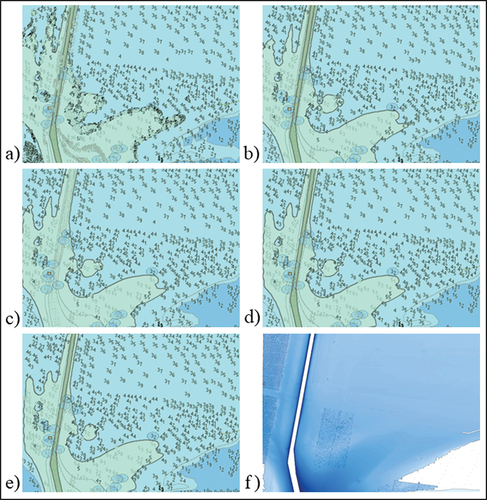
Contour displacement from generalization is evident in the northwestern region of each dataset, where a relatively deep valley recedes as smoothing iterations increase. Additionally, this occurs in the central-western area, where increased smoothing creates an isolated deep area. The contour generalization also significantly increases readability in these regions when comparing the linearly interpolated depth contour output (Figure 13(a)) with those that are smoothed (Figures 13(b–e). Additionally, there are regions of the area where no selectable soundings are present, namely in the west, south-central and southeast, which results in soundings not selected in those areas.

Across each dataset, there appears to be an east to west area where there is a gap in selected soundings and the density shifts from higher density in the south to lower density in the north. The area represents a slightly deeper and flatter region of the bathymetry, where additional soundings would be redundant. The soundings north of this area are primarily fill-radius soundings and those in the south are shoals. The southern region has more variability in depth compared to the north, which results in the identification of more shoal soundings. Furthermore, this is related to the precision of depth measurements and identification of the surface critical points. Local maxima (shoal soundings) are identified even if the difference in depth to neighboring soundings is only a centimeter. This is illustrated in Figure 14, where local maxima are shown in red, saddles in green, and minima in blue.

Figure 14. Depth precision and critical point identification.

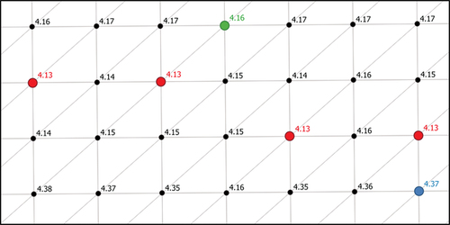
The quantity of critical points (and subsequent shoal, supportive, and deep soundings) could be reduced by first applying a shoal-bias rounding procedure to the depths to reduce the level of precision. For example, the depths of the two shoal soundings and those surrounding them (left, Figure 14) would convert from 4.13, 4.14, 4.15, etc. to 4.1, which would then result in these two soundings not being identified as local maxima. Conversely, increased measurement precision could exacerbate this issue.

6. Concluding remarks

This paper presented a cartographic sounding selection algorithm applied to variable quality multi-source bathymetry data that utilizes characteristics of both the DSM of the bathymetry and DCM of the ENC, a hierarchy and taxonomy of soundings, current ENC characteristics and features, and cartographic constraint correction procedures to produce a shoal-bias, near ENC-ready selection. The presented approach results in zero functionality violations, the most important for safe navigation, and minimizes legibility violations.

In this work, violations of the triangle test are used to assess functionality. Kastrisios et al. (2019b) demonstrated that there exists an intrinsic limitation with the triangle test, where selected soundings that significantly deviate from their expected value based on interpolation can still pass the IHO test. Accordingly, they developed the surface test to overcome this issue, which we use to select fill soundings in locations where depths cannot be easily visually interpolated by the mariner. We explored using the surface test over the triangle test to assess the functionality constraint; however, it was found that the test results in far too many violations, particularly in high quality data (e.g. CATZOC A1), which cannot be corrected without introducing significant legibility issues. These issues could be potentially mitigated by increasing the zoom on the ECDIS screen (or assigning them a different SCAMIN than the compilation scale); however, this is not the optimal viewing scale and relevant navigational features may be out of view as a result. Another approach would be to maintain these soundings in the ENC database and assign them a SCAMAX different than the compilation scale, so that they are displayed only when zoomed in, while also supporting ENC safety checks. Therefore, we tested and corrected the functionality constraint using the triangle test. Table 7 illustrates this issue, showing the number of surface test violations (shallow and deep) still present in the final cartographic selections.

Table 7. Surface test violations present in final cartographic sounding selections.

Dataset	Smoothing Iterations	Shallow Surface Test Violations	Deep Surface Test Violations	Total Surface Test Violations
New York Lower Bay, NY	0	795	3177	3972
	500	505	15,894	16,399
	1000	375	19,506	19,881
	1500	206	24,507	24,713
	2000	201	26,123	26,324
Galveston Bay, TX	0	117	428	545
	500	31	2492	2523
	1000	38	3230	3268
	1500	38	3830	3868
	2000	41	4311	4352
Mobile Bay, AL	0	285	342	627
	500	283	2369	2652
	1000	276	2939	3215
	1500	253	3738	3991
	2000	333	4365	4698
Savannah River and Calibogue Sound, SC	0	67	206	273
	500	20	852	872
	1000	8	1009	1017
	1500	0	3868	3868
	2000	0	1453	1453

It was also demonstrated how depth contours and existing bathymetric chart features can influence the final selection. We compared the results of our approach using linearly interpolated depth contours to those derived from a surface smoothed with shoal-bias. Generalizing depth contours in this manner can produce aesthetic and shoal-bias geometries at the cost of eliminating deep water. It is difficult to properly smooth a seabed or coastal area with varying topographies and waterway configurations using a single parameter, i.e. flat, high slope, narrow channel, or open water, because the contours are displaced differently under these conditions. Acknowledging the continued issues with contour generalization in nautical cartography, our approach accepts depth contours as input, which allows for the user to determine a satisfactory generalization prior to sounding selection. However, future work should explore using local metrics derived through an analysis of the underlying DSM to drive the smoothing operation to improve automation.

Fill sounding selection is a subjective process and the literature reinforces this, as numerous authors have proposed different methods. Our approach seeks to balance aesthetic and data-driven approaches; however, further research in this area is needed. The radius-fill approach used the current ENC as a reference to determine relative spacing between soundings. This assumes that the current ENC sounding distribution is optimal, which may not necessarily be the case due to a lack of a single industry accepted compilation workflow. Furthermore, a current ENC may not exist for certain areas and a trial-and-error approach would be required for determining radii lengths. Similar to depth contours, future work should investigate analyzing the bathymetric surface model to determine values for selecting radius-fill soundings. For example, using TIN edges to identify and delineate areas where small distances are observed (a channel) versus longer distances (e.g. channel entrance) and apply different rules accordingly (radii lengths). It was also observed that lower quality data resulted in fewer fill-surface soundings. These parameters could also be derived from a statistical analysis of the full ENC portfolio, as proposed by Kastrisios et al. (2023). This is due to that survey data of CATZOC “D” and “U” do not have a depth uncertainty tolerance, and as a result cannot be determined to be outside a certain level of accuracy. As data from unauthoritative sources becomes more prevalent, such as crowd-sourced bathymetry (IHO 2022), determining an appropriate tolerance for these data is required for future work.

We presented a cartographic selection algorithm to generalize bathymetry to a single scale. Future work should investigate using the methods described in this work, particularly assessing the DCM and constraint correction procedures, to continue generalizing through the scales. This should be expanded to other chart features for a fully automated solution.

Acknowledgements

We would like to thank the National Bathymetric Source team of the National Oceanic and Atmospheric Administration’s Office of the Coast Survey for providing us with the data used in this study.

Disclosure statement

No potential conflict of interest was reported by the author(s).

Data availability statement

The data and code supporting the findings of this study are available in figshare at https://doi.org/10.6084/m9.figshare.22735013

Additional information

Funding

The work of Christos Kastrisios was supported by the National Oceanic and Atmospheric Administration under [grant number NA20NOS4000196]. The work of Leila De Floriani was partially supported by the National Science Foundation under [grant number 1910766].

Notes on contributors

Noel Dyer

Noel Dyer is a PhD candidate in Geographical Sciences at the University of Maryland, College Park. His research interests include terrain data generalization and automated cartography.

Christos Kastrisios

Christos Kastrisios received his PhD degree from the National Technical University of Athens. He is currently a Research Assistant Professor at the University of New Hampshire Center for Coastal & Ocean Mapping.

Leila De Floriani

Leila De Floriani received her PhD degree from the University of Genova. She is currently a full professor at the University of Maryland, College Park, with a joint appointment with the Department of Geographical Sciences and University of Maryland Institute for Advanced Computer Studies (UMIACS).

Appendix

Table A1. Total filtered soundings before and after contour generalization.

Dataset	Total Original Source Soundings	Total Surrounding Source Soundings	Smoothing Iterations	Total Filtered Source Soundings	Total Filtered Surrounding Soundings
New York Lower Bay, NY	2,820,002	170,400	0	2,594,242	148,733
			500	2,585,157	128,056
			1000	2,581,694	126,156
			1500	2,578,962	123,159
			2000	2,576,537	120,356
Galveston Bay, TX	2,820,002	153,912	0	1,632,624	116,426
			500	1,525,808	102,318
			1000	1,491,104	90,799
			1500	1,467,371	81,549
			2000	1,445,967	74,536
Mobile Bay, AL	3,325,667	167,847	0	3,068,162	148,028
			500	3,040,379	144,519
			1000	3,032,047	143,491
			1500	3,026,019	142,988
			2000	3,020,898	142,658
Savannah River and Calibogue Sound, SC	3,156,773	162,833	0	1,805,803	92,511
			500	1,547,174	87,990
			1000	1,475,391	85,288
			1500	1,421,684	82,817
			2000	1,372,743	80,397

Table A2. CATZOC values of each sounding found in potentially selectable soundings (column five of Table A1).

Dataset	Smoothing Iterations	A1	A2	B	C	D/U
New York Lower Bay, NY	0	1,768,068	640,100	185,991	0	83
	500	1,767,784	640,041	177,251	0	81
	1000	1,767,056	639,734	174,824	0	80
	1500	1,766,026	639,320	173,536	0	80
	2000	1,765,174	638,680	172,603	0	80
Galveston Bay, TX	0	134,367	15,334	452,531	14	1,030,378
	500	126,224	15,334	392,450	11	991,789
	1000	123,322	15,334	377,859	5	974,584
	1500	120,984	15,334	366,572	3	964,478
	2000	118,627	15,334	355,842	2	956,162
Mobile Bay, AL	0	1,113,188	1,517,000	437,951	0	23
	500	1,113,188	1,517,000	410,168	0	23
	1000	1,113,188	1,517,000	401,836	0	23
	1500	1,113,188	1,517,000	395,808	0	23
	2000	1,113,188	1,517,000	390,687	0	23
Savannah River and Calibogue Sound, SC	0	0	0	445,986	1,339	1,358,478
	500	0	0	303,985	1139	1,242,050
	1000	0	0	281,423	982	1,192,986
	1500	0	0	267,037	863	1,153,784
	2000	0	0	255,435	786	1,116,522

Table A3. Sounding types found in legibility violations between individual soundings.

Dataset	Smoothing Iterations	Least Depth	Shoal	Deep	Supportive	Fill (Radius)	Fill (Surface)	Adjustment
New York Lower Bay, NY	0	1759	11	0	0	5	0	111
	500	34	11	0	0	4	0	46
	1000	29	7	0	0	5	2	40
	1500	24	7	0	0	5	0	39
	2000	16	10	0	0	5	0	42
Galveston Bay, TX	0	975	3	0	0	0	0	59
	500	3	2	0	0	1	0	7
	1000	1	6	0	0	1	0	10
	1500	1	5	0	0	0	0	3
	2000	1	5	0	0	0	0	3
Mobile Bay, AL	0	1165	0	0	0	0	0	19
	500	21	3	0	0	0	0	4
	1000	17	2	0	0	0	0	2
	1500	12	1	0	0	0	0	1
	2000	9	1	0	0	0	0	1
Savannah River and Calibogue Sound, SC	0	265	0	0	0	1	0	17
	500	7	1	0	0	0	0	14
	1000	4	1	0	0	0	0	12
	1500	2	1	0	0	0	0	7
	2000	0	1	0	0	0	0	5

Table A4. Summary of sounding types found in legibility violations with soundings and existing danger to navigation features.

Dataset	Smoothing Iterations	Least Depth	Shoal	Deep	Supportive	Fill (Radius)	Fill (Surface)	Adjustment
New York Lower Bay, NY	0	77	0	0	0	0	0	19
	500	24	0	0	0	0	0	25
	1000	23	0	0	0	0	0	24
	1500	21	0	0	0	0	0	25
	2000	20	0	0	0	0	0	25
Galveston Bay, TX	0	130	0	0	0	0	0	13
	500	4	0	0	0	0	0	11
	1000	4	0	0	0	0	0	8
	1500	3	0	0	0	0	0	9
	2000	1	0	0	0	0	0	10
Mobile Bay, AL	0	92	0	0	0	0	0	3
	500	2	0	0	0	0	0	1
	1000	2	0	0	0	0	0	3
	1500	2	0	0	0	0	0	4
	2000	0	0	0	0	0	0	2
Savannah River and Calibogue Sound, SC	0	10	0	0	0	0	0	7
	500	2	0	0	0	0	0	6
	1000	0	0	0	0	0	0	6
	1500	1	0	0	0	0	0	4
	2000	0	0	0	0	0	0	3

References

- Arundel, S. T., and G. Sinha. 2020. “Automated Location Correction and Spot Height Generation for Named Summits in the Coterminous United States.” International Journal of Digital Earth 13 (12): 1570–1584. https://doi.org/10.1080/17538947.2020.1754936.
- Baella, B., J. Palomar-Vázquez, J. E. Pardo-Pascual, and M. Pla. 2007. “Spot Heights Generalization: Deriving the Relief of theTopographic Database of Catalonia at 1: 25,000 from the Master Database.” The 7th ICA workshop on Progress in Automated Map Generalization. Moscow.
- Banchoff, T. 1970. “Critical Points and Curvature for Embedded Polyhedral Surfaces.” The American Mathematical Monthly 77 (5): 475–485.
- BLUETOPO. 2023. “BLUETOPO Data Specifications.” Accessed November 30, 2022. https://nauticalcharts.noaa.gov/data/bluetopo_specs.html.
- Brassel, K. E., and R. Weibel. 1988. “A Review and Conceptual Framework of Automated Map Generalization.” International Journal of Geographical Information System 2 (3): 229–244. https://doi.org/10.1080/02693798808927898.
- Calder, B. R., and L. A. Mayer. 2003. “Automatic Processing of High‐Rate, High‐Density Multibeam Echosounder Data.” Geochemistry, Geophysics, Geosystems 4 (6). https://doi.org/10.1029/2002GC000486.
- Chaudhry, O. Z., and W. A. Mackaness. 2008. “Creating Mountains Out of Mole Hills: Automatic Identification of Hills and Ranges Using Morphometric Analysis.” Transactions in GIS 12 (5): 567–589. https://doi.org/10.1111/j.1467-9671.2008.01116.x.
- Du, J. H., Y. Lu, and J. S. Zhai. 2001. “A Model of Sounding Generalization Based on Recognition of Terrain Features.” Proceedings of the 20th International Cartographic Conference, Beijing, China. August 6-10.
- Dyer, N., C. Kastrisios, and L. De Floriani. 2022. “Label-Based Generalization of Bathymetry Data for Hydrographic Sounding Selection.” Cartography and Geographic Information Science 49 (4): 338–353. https://doi.org/10.1080/15230406.2021.2014974.
- Environmental Systems Research Institute Documentation. 2023. “An Overview of the Maritime Toolbox.” Accessed November 30, 2022. https://pro.arcgis.com/en/pro-app/latest/tool-reference/maritime/an-overview-of-the-maritime-toolbox.htm.
- Gillies, S. “Shapely: Manipulation and Analysis of Geometric Objects.” 2007. Accessed November 30, 2022. https://github.com/Toblerity/Shapely.
- Guilbert, E. 2016. “Feature‐Driven Generalization of Isobaths on Nautical Charts: A Multi‐Agent System Approach.” Transactions in GIS 20 (1): 126–143. https://doi.org/10.1111/tgis.12147.
- Guilbert, E., and H. Lin. 2006. “B-Spline Curve Smoothing Under Position Constraints for Line Generalisation.” In Proceedings of the 14th annual ACM international symposium on Advances in geographic information systems, 3–10. https://doi.org/10.1145/1183471.1183474
- Guilbert, E., and E. Saux. 2008. “Cartographic Generalisation of Lines Based on a B‐Spline Snake Model.” International Journal of Geographical Information Science 22 (8): 847–870. https://doi.org/10.1080/13658810701689846.
- IHO (International Hydrographic Organization). 2017a. “IHO ECDIS Presentation Library. Edition 4.0. (2). Publication S-52. ANNEX a.” Monaco: International Hydrographic Organization.
- IHO (International Hydrographic Organization). 2017b. “Mariner’s Guide to Accuracy of Electronic Navigational Charts (ENC)., Edition 0.5. Publication S-67.” Monaco: International Hydrographic Organization.
- IHO (International Hydrographic Organization). 2017c. “Regulations of the IHO for International (INT) Charts and Chart Specifications of the IHO, Edition 4.7. Publication S-4.” Monaco: International Hydrographic Organization.
- IHO (International Hydrographic Organization). 2022. “Guidance to Crowdsourced Bathymetry, Edition 3.0.0. Publication B-12.” Monaco: International Hydrographic Organization.
- International Hydrographic Organization (IHO). 2014. IHO Transfer Standard for Digital Hydrographic Data. Supplementary Information for the Encoding of S-57., Edition 3.1. International Hydrographic Organization, Monaco.
- Janowski, L., R. Wroblewski, M. Rucinska, A. Kubowicz-Grajewska, and P. Tysiac. 2022. “Automatic Classification and Mapping of the Seabed Using Airborne LiDar Bathymetry.” Engineering Geology 301:106615. https://doi.org/10.1016/j.enggeo.2022.106615.
- Jingsheng, Z., and L. Yi 2005. “Recognition and Measurement of Marine Topography for Sounding Generalization in Digital Nautical Chart.” Marine Geodesy 28 (2): 167–174. https://doi.org/10.1080/01490410590953712.
- Kastrisios, C., and B. Calder. 2018. “Algorithmic Implementation of the Triangle Test for the Validation of Charted Soundings.” The 7th International Conference on Cartography and GIS, Sozopol, Bulgaria, June 18–23. https://doi.org/10.13140/RG.2.2.12745.39528.
- Kastrisios, C., B. Calder, G. Masetti, and P. Holmberg. 2019a. “On the Effective Validation of Charted Soundings and Depth Curves.” US Hydro. https://doi.org/10.13140/RG.2.2.18705.89440.
- Kastrisios, C., B. Calder, G. Masetti, and P. Holmberg. 2019b. “Towards Automated Validation of Charted Soundings: Existing Tests and Limitations.” Geo-Spatial Information Science 22 (4): 290–303. https://doi.org/10.1080/10095020.2019.1618636.
- Kastrisios, C., N. Dyer, T. Nada, S. Contarinis, and J. Cordero. 2023. “Increasing Efficiency of Nautical Chart Production and Accessibility to Marine Environment Data Through an Open-Science Compilation Workflow.” ISPRS International Journal of Geo-Information 12 (3): 116. https://doi.org/10.3390/ijgi12030116.
- Li, J. H., F. Wu, X. Y. Gong, J. W. Du, and R. X. Xing. 2018. “Depth Contour Smoothing Based on the Fitting of Multi-Segment Bezier Curves.” Marine Geodesy 41 (4): 382–404. https://doi.org/10.1080/01490419.2018.1465499.
- Li, M. Y., A. Zhang, D. J. Zhang, M. W. Di, and Q. J. Liu. 2021. “Automatic Sounding Generalization Maintaining the Characteristics of Submarine Topography.” IEEE Journal of Selected Topics in Applied Earth Observations & Remote Sensing 14:10278–10286. https://doi.org/10.1109/JSTARS.2021.3116997.
- Lovrinčević, D. 2019. “The Development of a New Methodology for Automated Sounding Selection on Nautical Charts.” Naše More 66 (2): 70–77. https://doi.org/10.17818/NM/2019/2.4.
- MacDonald, G. 1984. “Computer-assisted sounding selection techniques.” In The International Hydrographic Review. HYDRO 1982, Southhampton, England.
- NOAA (National Oceanic and Atmospheric Administration). 2021. “Nautical Chart Manual; Version 2021.3.” Silver Spring, MD, USA: U.S. Department of Commerce, Office of Coast Survey.
- Nyberg, J., S. Pe’eri, S. Catoire, and C. Harmon. 2020. “An Overview of the NOAA ENC Re-Scheming Plan.” International Hydrographic Review 24:7–20. https://journals.lib.unb.ca/index.php/ihr/article/view/33145.
- Oraas, S. R. 1975. “Automated Sounding Selection.” International Hydrographic Review.
- Palomar‐Vázquez, J., and J. Pardo‐Pascual. 2008. “Automated Spot Heights Generalisation in Trail Maps.” International Journal of Geographical Information Science 22 (1): 91–110. https://doi.org/10.1080/13658810701349003.
- Peters, R., H. Ledoux, and M. Meijers. 2014. “A Voronoi-Based Approach to Generating Depth-Contours for Hydrographic Charts.” Marine Geodesy 37 (2): 145–166. https://doi.org/10.1080/01490419.2014.902882.
- Rice G., K. Wyllie, R. Brennan, C. Koprowski, S. Wolfskehl, and Z. Burnett. 2020. “The National Bathymetric Source.” The Canadian Hydrographic Conference, Quebec City, Canada, February 24–27.
- Rocca, L., B. Jenny, and E. Puppo. 2017. “A Continuous Scale-Space Method for the Automated Placement of Spot Heights on Maps.” Computers & Geosciences 109:216–227. https://doi.org/10.1016/j.cageo.2017.09.003.
- Roth, R. E., C. A. Brewer, and M. S. Stryker. 2011. “A Typology of Operators for Maintaining Legible Map Designs at Multiple Scales.” Cartographic Perspectives 68:29–64. https://doi.org/10.14714/CP68.7.
- Ruas, A., and C. Plazanet. 1997. “Strategies for Automated Generalization.” Advances in GIS Research II: Proceedings of the Seventh International Symposium on Spatial Data Handling. London: Taylor and Francis.
- Rufat, D. 2022. “Triangle Python.” Accessed November 30, 2022. https://github.com/drufat/triangle.
- Rytz, A., E. Bantel, C. Hoinkes, G. Merkle, and G. Schelling. 1980 “Cartographic Generalization: Topographic Maps. Cartographic Publication Series (English Translation of Publication No.1)”. Swiss Society of Cartography.
- Samet, H. 1984. “The Quadtree and Related Hierarchical Data Structures.” ACM Computing Surveys (CSUR) 16 (2): 187–260. https://doi.org/10.1145/356924.356930.
- SevenCs. 2022. 7cs ENC Designer Version 4.7.0.14.
- Shewchuk, J. R. 1996. “Triangle: Engineering a 2D Quality Mesh Generator and Delaunay Triangulator.” Workshop on applied computational geometry, Berlin. https://doi.org/10.1007/BFb0014497
- Šiljeg, A., I. Marić, F. Domazetović, N. Cukrov, M. Lovrić, and L. Panđa. 2022. “Bathymetric Survey of the St. Anthony Channel (Croatia) Using Multibeam Echosounders (MBES)—A New Methodological Semi-Automatic Approach of Point Cloud Post-Processing.” Journal of Marine Science and Engineering 10 (1): 101. https://doi.org/10.3390/jmse10010101.
- Skopeliti, A., L. Stamou, L. Tsoulos, and S. Pe’eri. 2020. “Generalization of Soundings Across Scales: From DTM to Harbour and Approach Nautical Charts.” ISPRS International Journal of Geo-Information 9 (11): 693. https://doi.org/10.3390/ijgi9110693.
- Skopeliti, A., L. Tsoulos, and S. Pe’eri. 2021. “Depth Contours and Coastline Generalization for Harbour and Approach Nautical Charts.” ISPRS International Journal of Geo-Information 10 (4): 197. https://doi.org/10.3390/ijgi10040197.
- Smith, S. M. 2003. “The Navigation Surface: A Multipurpose Bathymetric Database.” Master diss., University of New Hampshire.
- Stateczny, A., C. Specht, M. Specht, D. Brčić, A. Jugović, S. Widźgowski, M. Wiśniewska, and O. Lewicka. 2021. “Study on the Positioning Accuracy of GNSS/INS Systems Supported by DGPS and RTK Receivers for Hydrographic Surveys.” Energies 14 (21): 7413. https://doi.org/10.3390/en14217413.
- Stoter, J., M. Meijers, P. van Oosterom, D. Grünreich, and M. Kraak. 2010 “Applying DLM and DCM Concepts in a Multi-Scale Data Environment.” Proceedings of GDI 2010: symposium on generalization and data integration, Boulder, Colorado.
- Sui, H. G., P. G. Cheng, A. M. Zhang, and J. Y. Gong. 1999. “An Algorithm for Automatic Cartographic Sounding Selection.” Geo-Spatial Information Science 2 (1): 96–99. https://doi.org/10.1007/BF02826726.
- Sui, H. G., X. Y. Zhu, and A. M. Zhang. 2005. “A System for Fast Cartographic Sounding Selection.” Marine Geodesy 28 (2): 159–165. https://doi.org/10.1080/01490410590953695.
- Szafarczyk, A., and C. Toś. 2022. “The Use of Green Laser in LiDar Bathymetry: State of the Art and Recent Advancements.” Sensors 23 (1): 292. https://doi.org/10.3390/s23010292.
- Tsoulos, L., and K. Stefanakis. 1997. ““Sounding Selection for Nautical Charts: An Expert System Approach.” the18th International Cartographic Conference, Sweden, June 23–27.
- Weintrit, A. 2018. “Clarification, Systematization and General Classification of Electronic Chart Systems and Electronic Navigational Charts Used in Marine Navigation. Part 2-Electronic Navigational Charts.” TransNav: International Journal on Marine Navigation and Safety of Sea Transportation 12 (4): 769–780. https://doi.org/10.12716/1001.12.04.17.
- Yu, W. H. 2018. “Automatic Sounding Generalization in Nautical Chart Considering Bathymetry Complexity Variations.” Marine Geodesy 41 (1): 68–85. https://doi.org/10.1080/01490419.2017.1393476.
- Zhang, X., and E. Guilbert. 2011. “A Multi-Agent System Approach for Feature-Driven Generalization of Isobathymetric Line.” Advances in Cartography and GIScience 1:477–495. https://doi.org/10.1007/978-3-642-19143-5_27.
- Zoraster, S., and S. Bayer. 1992. “Automated Cartographic Sounding Selection.” International Hydrographic Review.