Spatiotemporal imagery selection for full coverage image generation over a large area with HFA-Net based quality grading

ABSTRACT

Remote sensing images often need to be merged into a larger mosaic image to support analysis on large areas in many applications. However, the performance of the mosaic imagery may be severely restricted if there are many areas with cloud coverage or if these images used for merging have a long-time span. Therefore, this paper proposes a method of image selection for full coverage image (i.e. a mosaic image with no cloud-contaminated pixels) generation. Specifically, a novel High-Frequency-Aware (HFA)-Net based on Swin-Transformer for region quality grading is presented to provide a data basis for image selection. Spatiotemporal constraints are presented to optimize the image selection. In the temporal dimension, the shortest-time-span constraint shortens the time span of the selected images, obviously improving the timeliness of the image selection results (i.e. with a shorter time span). In the spatial dimension, a spatial continuity constraint is proposed to select data with better quality and larger area, thus improving the radiometric continuity of the results. Experiments on the GF-1 images indicate that the proposed method reduces the averages by 76.1% and 38.7% in terms of the shortest time span compared to the Improved Coverage-oriented Retrieval algorithm (MICR) and Retrieval Method based on Grid Compensation (RMGC) methods, respectively. Moreover, the proposed method also reduces the residual cloud amount by an average of 91.2%, 89.8%, and 83.4% when compared to the MICR, RMGC, and Pixel-based Time-series Synthesis Method (PTSM) methods, respectively.

KEYWORDS:

• Image selection
• spatiotemporal constraints
• full coverage image generation
• High-Frequency-Aware (HFA)-Net
• regional quality grading

1. Introduction

Mosaic images play a vital role in the analysis of transregional remote sensing images (Yuan et al. 2023). They are formed by merging remote sensing images of interest (Chu, Jiang, and Cheng 2014) and have been widely used to support analyses over large areas in many applications, e.g. environmental monitoring (Theodomir et al. 2022), agricultural estimation (Tariq et al. 2022), and smart cities (Li, Wang, and Jiang 2021). In the process of generating mosaic images, image selection is one of the key steps, and its role is to select suitable source images according to the application requirements.

With the rapid development of earth observation technology, an increasing number of satellites can provide massive remote sensing images. However, more data is not always better, especially in mosaic applications (Eken and Sayar 2021) where the use of an excessive number of images beyond what is required can result in unnecessary computation costs. Meanwhile, commonly used methods that reduce the number of selected results based on metadata information may not guarantee full coverage of the target area. Moreover, images obtained at different times may exhibit radiometric inconsistencies due to uncertainties in at-sensor radiances caused by variations in view angle, sunlight angle (Wang et al. 2022), atmospheric conditions (Geng et al. 2020), and Bidirectional Reflectance Distribution Function (BRDF) (Roy et al. 2016).

Currently, many applications require mosaic images with not only higher image quality but also better timeliness (Michele et al. 2019). However, on the one hand, remote sensing images are often affected by clouds, which can lead to missing information in the images (Chen, Pan, and Zhang 2023); on the other hand, if only cloudless images are used, images with longer time spans might have to be selected to cover the application area entirely. For example, the time span of the global 14.25 m mosaic image generated by NASA’s GeoCover 2000 project is up to 3 years (NASA, 2016). It may not meet the needs of many applications, e.g. annual monitoring for the Poyang Lake wetland (Chen et al. 2018) and annual analysis of land cover for urban areas (Liu et al. 2019). Therefore, it is crucial to select images with better timeliness and high-quality from the massive remote sensing data to support full coverage image generation over a large area to meet the requirements of various applications.

Many previous studies have been conducted on image selection. There are three kinds of methods: image-based methods, tile-based methods, and pixel-based methods. Image-based methods take a single image as a unit to evaluate the quality and select images with better quality. For instance, Miao et al. (2010) and Xue et al. (2013) studied the fast query technique of multisource data based on spatial location. Yan et al. (2022) proposed an improved coverage-oriented retrieval algorithm that aims to retrieve an optimal image combination with the minimum number of images closest to the imaging time of interest while maximizing covering the target area. Li et al. (2017) presented a screening model based on normalized mathematical calculations that uses parameters such as imaging time, cloud cover, and resolution, which can effectively remove data with earlier time-phases, repeated coverage, and high cloud cover. Tile-based methods divide images according to certain rules in time, space, and other dimensions, forming a series of tiles. The commonly used is the five-layer and fifteen-level data grading organization model (Lai et al. 2013). Rao (2019) presented a full coverage retrieval method of remote sensing data based on grid compensation, which can quickly and accurately acquire cloud-free data covering a specific area. Since tile mode had further increased the scale of data and placed significant pressure on data retrieval, Zuo et al. (2018) studied a comprehensive retrieval strategy. This strategy automatically retrieves remote sensing tile data that meets practical application requirements from a large amount of data, using full coverage, spatial data distribution, and single-grid temporal retrieval. Liu et al. (2008) studied image selection methods based on spatial relationships and semantic features, which reduce retrieval complexity and improve retrieval accuracy. Pixel-based methods take the pixel as a unit, and the value of each pixel is determined according to certain rules based on multiple images in the same area. When one pixel is covered by multiple images at different imaging times, its value is calculated using certain criteria, such as the maximum, minimum, median, or weighted value. NASA’s Web-enabled Landsat Data project adopted the pixel-based time series synthesis method. It used 6521 Landsat Enhanced Thematic Mapper Plus data acquisitions gathered between December 2007 and November 2008 to generate mosaics of the conterminous United States on a monthly, seasonal, and annual basis (Roy et al. 2010). Pixel-based methods share similarities with various video splicing methods in computer vision. Many computer vision video stitching algorithms can be used to obtain synthetic cloudless images (Hsu and Tsan 2004; Wexler, Shechtman, and Irani 2007). Cloud cover is a common problem (King et al. 2013) in remote sensing imagery (Zhang et al. 2021). However, in the image-based methods, many images are discarded due to excessive cloud. There are still many cloudless areas even in images with a large percent of cloud coverage areas. If these cloudless areas can be used, the utilization rate of images and the timeliness of selection results could be further improved. In the tile-based methods, most did not use the data of the same image to the greatest extent in a local area, which could cause the phenomenon of the discontinuity of ground features in the final full coverage images. In the pixel-based methods, the values of adjacent pixels can come from different images, which could cause many discontinuous parts in the final merged image. Moreover, the time span of the final merged image might not be optimal.

Different from these methods, this paper proposes a novel image selection method for full coverage image (i.e. a mosaic image with no cloud-contaminated pixels, it is to say that each pixel in full coverage image is a valid coverage of the earth’s surface) generation over a large area. The presented method involves proposing a new High-Frequency-Aware (HFA)-Net to grade the quality of images, providing the foundational data for image selection. In the HFA-Net, the Swin-Transformer effectively utilizes multi-scale spatial details and high-level semantic information. Additionally, a High-Frequency Module (HFM) is proposed to extract high-frequency features and a Feature Fusion Module (FFM) is used for determining different importance to features by weighting each feature channel adaptively to improve the quality grading performance. Quality grading is conducted at the block (256 $\times$ 256) level, which means the block is the smallest unit used for grading. The presented method maximizes the utilization of cloud-free areas within cloudy images through quality grading. This significantly reduces image wastage compared to using only completely cloud-free images. Subsequently, spatiotemporal constraints are presented to further optimize image selection. Adjacent blocks with the same quality level after grading are dynamically clustered into larger regions. These regions are treated as units for the next stage of selection. Specifically, the shortest-time-span constraint is applied to shorten the time span of the selected images used for generating full coverage images, thereby improving the timeliness of results. Additionally, a spatial continuity constraint is used to select data (the regions clustered by blocks) with better quality and larger area, enhancing the radiometric continuity of the image selection results.

A comparison of the proposed method with previous methods is shown in Table 1. The comparison items include considering cloud, considering timeliness, and considering radiometric continuity. “$\surd$” represents the item is fully considered. “$\times$” represents the item is not considered.

Table 1. A comparison of the presented method with previous methods.

Method	Scale	Considering cloud	Considering timeliness	Considering radiometric continuity
Image-based methods	Image	$\surd$	$\times$	$\surd$
Tile-based methods	Tile	$\surd$	$\times$	$\times$
Pixel-based methods	Pixel	$\surd$	$\times$	$\times$
The presented method in this manuscript	Tile	$\surd$	$\surd$	$\surd$

This study proposes an image selection method for full coverage image generation over a large area with HFA-Net based quality grading. It aims to select data with better timeliness and high-quality from massive remote sensing data, thereby providing support for generating full coverage images over a large area that meet practical application requirements.

The remainder of this paper is organized as follows. Section 2 presents the complete details of the proposed method. Section 3 provides comprehensive experimental results. Section 4 draws the conclusions.

2. Methodology

The image selection of the presented method is established on the foundation of quality grading of images by blocks. The HFA-Net network model based on the Swin-Transformer is proposed to improve the quality grading performance. During image selection, in the temporal dimension, the shortest time span is determined using the Uniform Cost Search (UCS, a cost-based graph search strategy utilized to discover the path with the lowest cost within a graph) strategy (Mansour, Eid, and Elbeltagi 2022) while considering the Time of Interest (TOI, a specific time that users focus on). Then, it is used as a constraint to enhance the timeliness of the image selection results. In the spatial dimension, a spatial continuity constraint is utilized to select regions with better quality and larger area to improve the radiometric continuity of the image selection results.

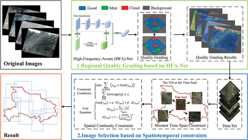
The flowchart of the presented method is shown in Figure 1. It consists of two main steps, namely, regional quality grading and image selection. In Figure 1, the green box is the architecture of the regional quality grading. The quality of images is set to four levels, namely, good (blue), mist (green), cloud (red), and background (gray). The quality of each image is graded by blocks using HFA-Net. Subsequently, adjacent blocks with the same quality level are dynamically clustered using the region growing algorithm (Sahoo et al. 2015) and the quality grading results are obtained. The blue box is the architecture of the image selection. In this step, the inputs are image subsets obtained based on the results of regional quality grading. Then, the UCS algorithm is used to find the shortest time span, and the spatial continuity constraint is used to find the data with better quality and larger area. Specifically, the shortest time span is determined based on the selected TOI (as the time seed). Then, the data are selected from the quality grading results to construct a candidate dataset based on the shortest-time-span constraint. Finally, the candidate dataset is optimized through the spatial continuity constraint to obtain the image selection results.

Figure 1. Flowchart of the presented spatiotemporal imagery selection method.

2.1. Regional quality grading based on HFA-Net

Cloud cover has a significant impact on remote sensing images. To reduce the impact of clouds and improve the utilization rate of data, the region quality grading algorithm based on HFA-Net network model is proposed. Images are graded by blocks, and each block is classified into a different quality level. Then, adjacent blocks with the same quality level are dynamically clustered into larger regions for subsequent experiments.

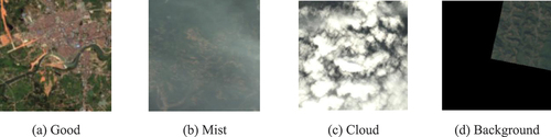
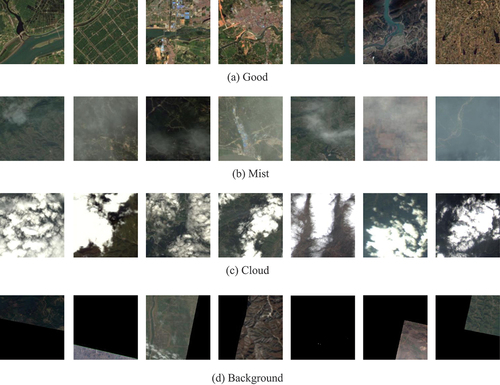
In order to select the data for full coverage image generation, the quality of images is classified into four quality levels (as shown in Figure 2). When the land surface is clearly visible and no cloud covering, the quality level is Good. When the land surface is relatively clear but obscured by thin clouds, the quality level is Mist. When parts of the land surface are completely covered by thick clouds and ground objects are invisible, the quality level is Cloud. When the image contains background pixels, it is categorized into Background. The fact is that images of different quality levels all have both high-frequency features (Luo et al. 2021) and low-frequency features (Li et al. 2022). However, in convolutional neural networks, high-frequency features are gradually blurred with convolution operations and down-sampling. Therefore, in this paper, high-frequency features are extracted to enhance the difference between images of different quality levels, thereby improving the quality grading performance.

Figure 2. Example diagrams for the categories. (a) Represents the ‘Good’ level; (b) represents the ‘Mist’ level; (c) represents the ‘Cloud’ level; (d) represents the ‘Background’ level.

In the paper, HFA-Net is proposed as a new network model for image quality grading, constructed based on improvements made to the Swin-Transformer. The Swin-Transformer is employed as one of the submodules within HFA-Net. Specifically, HFA-Net comprises three distinct modules: the Swin-Transformer module, the HFM, and the FFM. Within the HFA-Net framework, the Swin-Transformer serves as the backbone for extracting features, the HFM is used to obtain high-frequency features, and the FFM is employed for fusing the extracted features. In the field of remote sensing image quality grading, traditional methods rely on manually crafted features, which may overlook many feature variations. Additionally, they encounter challenges when processing large high-resolution images due to computational demands. However, the Swin-Transformer (Liu et al. 2021) has the capacity to address these issues. It utilizes a phased windowed self-attention mechanism to effectively capture features at different scales and resolutions in remote sensing images, thereby enhancing grading accuracy. Furthermore, the end-to-end nature of the Swin-Transformer enhances its own generalization capability. Therefore, the Swin-Transformer is used as the backbone of HFA-Net. Then, HFA-Net introduces the HFM and the FFM to make full use of different features. High-frequency features are important for image quality grading. Inspired by the previous research (Zhang et al. 2022), a trainable Laplacian operator has been introduced to extract high-frequency features.

In the field of deep learning, shallow-layer (Venetsanos et al. 2003) refers to the segment of a neural network with fewer layers. A neural network believed to have just one hidden layer (or none) is called a shallow neural network. Features extracted by shallow networks are termed shallow-layer features, containing more positional and detailed information. Deep-layer (Montavon, Samek, and Müller 2018) refers to the section of a neural network with multiple layers. A neural network with two or more hidden layers is considered a deep neural network. Features extracted by deep networks are called deep-layer features, containing more high-level semantic information. Specifically, four layers of features can be obtained from the Swin-Transformer backbone. The features of the first (shallow) and last (deep) layers of the backbone are input into the HFM to obtain two complementary high-frequency features. Then, shallow-layer high-frequency features and deep-layer high-frequency features are concatenated together as the final high-frequency features. Finally, the high-frequency features and the last-layer features of Swin-Transformer are fused in FFM and the quality grading results can be obtained. The structure of the HFA-Net network model is shown in Figure 3.

Figure 3. Structure of the HFA-Net network model.

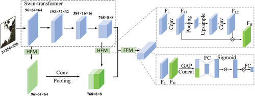
Features of Swin-Transformer ($F_L$) are taken as the input of HFM. First, a 1 $\times$ 1 convolutional layer is employed to obtain the original low frequency features $F_{L1}$. Then, a pooling layer is used to obtain low-resolution features. After up-sampling and passing through a 1 $\times$ 1 convolutional layer, the $F_{L2}$ with recovered resolution is obtained. Finally, high-frequency features are got by the subtraction between $F_{L1}$ and $F_{L2}$ (Equation (1)(1) $F_H=F_{L1}-F_{L2}$(1) ). This design ensures the high-frequency features extraction in a trainable manner.

(1) $F_H=F_{L1}-F_{L2}$(1)

High-frequency features and low-frequency features play different roles in the assessment of image quality. Inspired by the researches (Hu, Shen, and Sun 2018), a FFM (as shown in Figure 3) is introduced to better incorporate high-frequency features. First, high-frequency features $F_H$ and low-frequency features $F_L$ are operated with Global Average Pooling (GAP), and then concatenated in the channel direction. Afterward, the weights of each channel can be obtained by Fully Connected (FC) layers and the sigmoid function. The weights are multiplied and summed with the concatenated features. Finally, a FC layer is used to make the output channels equal to the number of quality grading classes. In this way, both high-frequency and low-frequency features are effectively leveraged.

To select the most suitable network model for quality grading, HFA-Net is evaluated on GaoFen-1 (GF-1) satellite remote sensing images by comparing with other commonly used network models for image classification. These models include AlexNet (Christian and Rottensteiner 2020), VGG-19 (Simonyan and Zisserman 2014), WideResNet (WRN)-101-2 (Zagoruyko and Komodakis 2016), ResNet-50 (He et al. 2016), DenseNet-169 (Gao et al. 2017), ResNeXt-101 (Xie et al. 2017), Res2Net (Gao et al. 2021), and Swin-Transformer (Liu et al. 2021). HFA-Net is trained by Adam optimizer (${\rho }_1=0.9$, ${\rho }_2=0.999$, weight decay $=$ 0.0005). The initial learning rate is set to 1e-3 and divided by ten every 30 epochs. The batch size is set to 32, and the training epoch is set to 100. The model is implemented by PyTorch. The Overall Accuracy (OA) (Prins and Niekerk 2021) is used to quantify the grading results. The metric of OA is defined as follows.

(2) $\begin{array}{c}OA=\frac{{\sum }_{k=1}^N{x}_{kk}}{{\sum }_{i=1}^N{\sum }_{j=1}^N{x}_{ij}}\end{array}$(2)

where ${\sum }_{k=1}^N{x}_{kk}$ represents the total number of correctly graded samples, ${\sum }_{i=1}^N{\sum }_{j=1}^N{x}_{ij}$ represents the total number of samples.

The accuracy results of different models are shown in Figure 4, where the abscissa represents the accuracy and the ordinate represents the model’s name.

Figure 4. Accuracy comparison of different models.

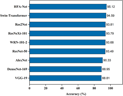
As shown in Figure 4, HFA-Net network model achieves better performance on the dataset. Furthermore, ablation studies of HFM and FFM are performed. Table 2 shows the quantitative performance of three groups of experiments: (a) quality grading only using Swin-Transformer; (b) quality grading using Swin-Transformer and HFM; (c) quality grading using HFA-Net, which includes Swin-Transformer, HFM and FFM.

Table 2. Quantitative performance of ablation experiments.

Methods	Backbone	Feature schemes	Fusion schemes	OA (%)
(a)	Swin-Transformer	$\times$	$\times$	94.59
(b)	Swin-Transformer	HFM	$\times$	94.96
(c)	Swin-Transformer	HFM	FFM	95.12

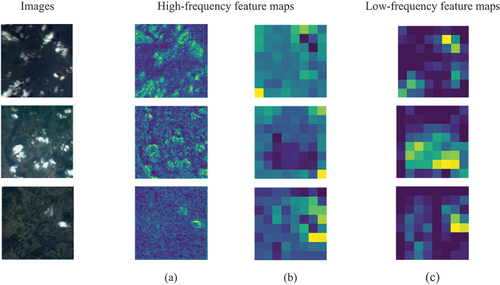
Experiment (b) adopts HFM to utilize high-frequency features compared to experiment (a). OA is improved by close to 0.4%, which proves the effectiveness of extracted high-frequency features. The OA of experiment (c) is improved by nearly 0.6% than that of experiment (a). It indicates that the introduction of high frequency features and the fusion of high and low frequency features can improve the quality grading performance. To intuitively demonstrate the effectiveness of high-frequency features, the low-frequency and high-frequency feature maps are exhibited. High-frequency features are important to capture the diversity within a class and the similarity between classes (Zhang et al. 2022). During the process of extracting low-frequency features, textures cannot be effectively retained through hierarchical filtering and down-sampling operators. In contrast, the extracted high-frequency features place a particular emphasis on texture information, thereby exhibiting more distinct features between the target and the background. As shown in Figure 5, there are two high-frequency and one low-frequency feature maps, with the high-frequency features highlighting the texture.

Figure 5. Comparison of low-frequency and high-frequency feature maps at the ‘cloud’ level. (a) represents the high-frequency features extracted from the first layer of the backbone; (b) represents the high-frequency features extracted from the last layer of the backbone; (c) represents the low-frequency features extracted from the last layer of the backbone.

2.2. Image selection based on spatiotemporal constraints

In this paper, a selection algorithm based on spatiotemporal constraints is proposed. In the selection process, the shortest-time-span constraint is used to shorten the time span of the image selection results. Subsequently, a spatial continuity constraint is used to select data with better quality and larger area to improve the radiometric continuity of the image selection results.

2.2.1. Shortest-time-span constraint

Timeliness is a significant concern in practical applications. Therefore, the shortest-time-span constraint is proposed to improve the timeliness of the select results as much as possible. The constraint aims to determine the shortest time span while prioritizing the data of high quality and ensuring full coverage of the target area. It is carried out through the Spatial Grid Marking (SGM) and the UCS strategy. After the shortest time span is determined, the data imaged within that span are selected to form a candidate dataset for subsequent experiments.

SGM consists of two parts: grid construction and grid marking. For grid construction, the target area is divided into equidistant grids based on the smallest circumscribed rectangle of it. For grid marking, the first step is to traverse images in the dataset in a certain order. Then, each grid is judged whether it is covered. The third step is remarking the grids that meet the conditions and recording the current image. In fact, the entire grids form a state matrix reflecting whether each corresponding grid is covered. If all grids are marked, the target area will be covered fully.

Given that the order of images can significantly impact the results, the UCS strategy (a directional and purposeful search algorithm) is adopted to optimize the selection order. The UCS strategy has high selection efficiency and can obtain results that meet the requirement in a relatively short time. At the same time, this paper has made improvements based on the actual situation: the TOI is taken as the starting point, and the time interval is taken as the path cost.

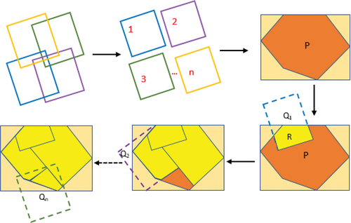
The schematic diagram of data selection based on the constraint is shown in Figure 6. As shown in Figure 6, the TOI is used as a condition to arrange the images in order. Then, the subsequent grid mark processing is performed based on this order of images. The arbitrary polygon $P$ (the brown rectangle) represents the spatial geometric object of the selected area. The enclosing rectangle of $P$ is shown in the orange rectangle. The effective range polygon of the image to be selected is $Q_i$ (the dotted rectangle. $0<i<n+1$, where $n$ is the total number of images of the candidate image set). $R$ (The yellow rectangle) is the intersection area of the selected area polygon $P$ and the image effective range polygon $Q_i$, namely, $R=\left\{X|X\in P,\mathrm{a}\mathrm{n}\mathrm{d}X\in Q_i\right\}$. If the selected area $P$ is all marked finished, the full coverage selection is complete. In other words, the target region is completely covered, the time span of the set $R$ is the shortest time span that satisfies full coverage requirements, and $R$ is the candidate dataset.

Figure 6. Data selection based on the shortest-time-span constraint.

2.2.2. Spatial continuity constraint

Radiometric continuity means that the values of pixels in an image should reflect ground features as continuously as possible, while avoiding fragmented or artificially created edges. To improve the radiometric continuity of image selection results, the spatial continuity constraint is proposed. The spatial continuity constraint means the constraint to select adjacent pixels within an image as many as possible. It consists of two parts: minimizing the cumulative sum of the total path cost and ensuring that the image selection results cover the target area entirely. It is defined as Equation (3)(3) $\begin{array}{c}\left\{\begin{array}{c}min\sum _{⟨p,q⟩\in Q}\left(x_{pq}\times Cost\left(x_{pq}\right)\right)\\ \sum _{q\in Q}\mathrm{C}\mathrm{o}\mathrm{v}\mathrm{e}\mathrm{r}\mathrm{a}\mathrm{g}\mathrm{e}\left(q\right)\ge L\end{array}\right.\end{array}$(3) .

In a directed graph $G=\left(Q,X,A,T\right)$, where $Q=\left\{q_1,q_2,\dots ,q_n\right\}$ is the set of images in the network, $X=\left\{x_{pq};p,q\in Q\right\}$ is the set of edges, $A$ is the spatial attribute function, and $T$ is the time attribute function. The goal of the spatial continuity constraint is to find a path from a starting point to an endpoint within a given full coverage target, and the path has minimal cost. The above constraint conditions can be expressed as follows.

(3) $\begin{array}{c}\left\{\begin{array}{c}min\sum _{⟨p,q⟩\in Q}\left(x_{pq}\times Cost\left(x_{pq}\right)\right)\\ \sum _{q\in Q}\mathrm{C}\mathrm{o}\mathrm{v}\mathrm{e}\mathrm{r}\mathrm{a}\mathrm{g}\mathrm{e}\left(q\right)\ge L\end{array}\right.\end{array}$(3)

where $x_{pq}\times Cost\left(x_{pq}\right)$ is the path cost of $x_{pq}$, $x_{pq}$ is the symbol for whether edge $⟨p,q⟩$ exists in a path, which is a Boolean value, $p$ and $q$ represent images, and $\mathrm{C}\mathrm{o}\mathrm{v}\mathrm{e}\mathrm{r}\mathrm{a}\mathrm{g}\mathrm{e}\left(q\right)$ represents the coverage of image $q$.

In the process of path cost calculation, the temporal and spatial dimensions have been processed simultaneously, considering each image’s temporal and spatial attributes. Therefore, the cost of each image is defined as the sum of the cost in the temporal and spatial dimensions. The cost can be expressed in Equation (4)(4) $\begin{array}{c}\left\{\begin{array}{c}Cost\left(x_{pq}\right)=\alpha \cdot T\left(x_{pq}\right)+\beta \cdot A\left(x_{pq}\right)\\ T\left(x_{pq}\right)=\frac{\left|t_p-t_q\right|}{t_{\mathrm{s}\mathrm{p}\mathrm{a}\mathrm{n}}}\\ A\left(x_{pq}\right)=1-{\left(\frac{are{a}_q}{are{a}_{\mathrm{m}\mathrm{a}\mathrm{x}}}\right)}^n\end{array}\right.\end{array}$(4) .

(4) $\begin{array}{c}\left\{\begin{array}{c}Cost\left(x_{pq}\right)=\alpha \cdot T\left(x_{pq}\right)+\beta \cdot A\left(x_{pq}\right)\\ T\left(x_{pq}\right)=\frac{\left|t_p-t_q\right|}{t_{\mathrm{s}\mathrm{p}\mathrm{a}\mathrm{n}}}\\ A\left(x_{pq}\right)=1-{\left(\frac{are{a}_q}{are{a}_{\mathrm{m}\mathrm{a}\mathrm{x}}}\right)}^n\end{array}\right.\end{array}$(4)

where $T\left(x_{pq}\right)$ is defined as the temporal dimension function, $A\left(x_{pq}\right)$ is defined as the spatial dimension function, and $t_p$ and $t_q$ are the imaging times of $p$ and $q$, respectively. Here, $t_{\mathrm{s}\mathrm{p}\mathrm{a}\mathrm{n}}$ is the shortest time span, $are{a}_{\mathrm{m}\mathrm{a}\mathrm{x}}$ represents the maximum area, and $are{a}_q$ represents the area of image $q$. The smaller the path cost is, the greater the probability of an image being selected. To preferentially select images with larger areas, $A\left(x_{pq}\right)$ is set to be a quadratic function. The dependent variable changes faster when the independent variable increases. Here, $n$ in $A\left(x_{pq}\right)$ is a natural number greater than 1, and it is set to 2 based on experience. The value range of $T\left(x_{pq}\right)$ is set as (0, 1], namely, 0 non-inclusive to 1 inclusive. The value range of $A\left(x_{pq}\right)$ is set to [0, 1), namely, 0 inclusive to 1 non-inclusive. Additionally, $\alpha$ and $\beta$ are the weights in the temporal dimension and the spatial dimension, respectively. The weight values are all set to 0.5.

In spatial continuity constraint process, a priority queue (Xu et al. 2014) is used to store the node states. A given starting node $p$ is generated first, and then, the cost value $Cost\left(x_{pq}\right)$ between the image $p$ and the image $q$ is calculated to initialize the priority queue. The image with the lowest cost is selected first to judge the constraint conditions. If the conditions are met, it is added to the set $L$ and removed from the queue. Then, the starting node is updated, and the cost value of each node image is recalculated. The loop continues until the end condition of the loop is triggered. Finally, the result set $L$ is output.

3. Experiments

3.1. Experimental data

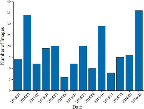
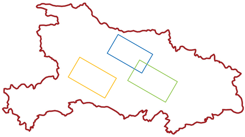
The experimental area is Hubei Province, which is in central China (29°01′53″N ~ 33°6′47″N, 108°21′42″E ~ 116°07′50″E). The total area of it is 185,900 km². In the experiments, data are GF-1 satellite (Li et al. 2021) remote sensing images with a resolution of 16 m, and a total of 251 images (17,849 $\times$ 15,883) (as shown in Figure 7) were used. The specific imaging time distribution of the data is shown in Figure 8.

Figure 7. GF-1 data of Hubei Province from January 2015 to March 2016.

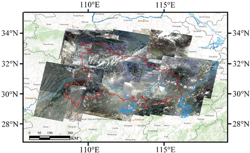
Figure 8. Imaging time distribution of data.

3.2. Regional quality grading experiments

A dataset that contained four types, including Good, Mist, Cloud, and Background, was constructed for HFA-Net training. To ensure representativeness, the dataset includes images from different latitudes in China. It comprises 50,000 images (256 $\times$ 256) clipped from the 251 radiometrically corrected GF-1 images. The numbers of Good, Mist, Cloud, and Background are 24,600, 11,850, 11,095 and 2455, respectively. Some representative images are shown in Figure 9. The ratio of training set to validation set is 4:1.

Figure 9. Some examples of annotated dataset. (a) represents the ‘Good’ level; (b) represents the ‘Mist’ level; (c) represents the ‘Cloud’ level; (d) represents the ‘Background’ level.

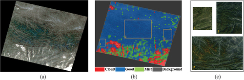
Then the trained HFA-Net was used to rate the 251 GF-1 images. A result example is shown in Figure 10. Figure 10(a) shows the original image and Figure 10(b) displays the grading result. In the grading display, red represents the cloud-covered area in the image, green represents the mist area, blue represents the good area, and gray represents the background area. According to the grading results, adjacent blocks with the same quality level in the image were dynamically clustered into larger regions. Then, regions were extracted as regular rectangles, which is good for matching during the grid marking process. These regions with better quality (as shown in Figure 10(c)) were extracted for the subsequent experiments.

Figure 10. (a) Original image. (b) Region quality grading result. (c) Some examples of ‘Good’ regions.

3.3. Image selection experiments

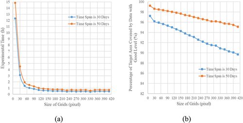
To explore the impact of grid size on the image selection performance, experiments were conducted using grids of various sizes. Experimental results are shown in Figure 11. In Figure 11(a), the abscissa represents the size of grids (the unit is pixel), and the ordinate represents the experimental time (the unit is hour). In Figure 11(b), The abscissa is the same as that of Figure 11(a), and the ordinate represents the percentage of target area covered by data with “Good” level. The time span in the experiments is set to 30 days for the first time and to 50 days for the second time. In the same time span, smaller grid sizes require more time to process, but result in a larger coverage ratio of data with “Good” level. Therefore, to achieve a balance between time efficiency and coverage ratio, the size of grids is set to 100 $\times$ 100 in this manuscript.

Figure 11. Experimental results. (a) Relationship between the size of grids and the experimental time; (b) relationship between the size of grids and the percentage of target area covered by data with ‘Good’ level.

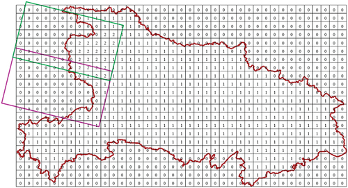
In the image selection experiments, the smallest bounding rectangle of Hubei Province was obtained and divided at equal intervals. In Figure 12, the grid values in and out of Hubei Province were marked as 1 and 0, respectively. If the grid is within the valid range of the image and has a value of 1, its value is re-marked to 2 and the current image was retained. By analogy, full coverage selection was accomplished when all grids with a value of 1 were marked as 2, and the image set retained in the process was the result.

Figure 12. Schematic diagram of image overlay grid marking.

In the step of finding the shortest time span, the UCS strategy was adopted to consider the user’s requirements for TOI. It used the TOI as the starting point of the search, utilized the imaging time interval as the path consumption, and then searched forward (backward) based on path cost from small to large. For example, when the TOI is 1 February 2016, then it would serve as the time seed. The shortest time span that meets the full coverage of the whole region was found to be 53 days. Then, images in the shortest time span range were optimally selected by considering the spatial continuity constraint. As shown in Figure 13, the crimson area is the administrative region of Hubei Province, and the polygons represented by other colors are the valid range polygons of the images. The image (blue rectangle) was processed at first because it has a minimal cost value. The next image (green rectangle) processed had the second smallest cost value. The results when the stop condition triggers (full coverage of Hubei Province) were the image selection results.

Figure 13. Schematic diagram of the spatial continuity constraint algorithm.

3.4. Experimental results and analysis

To verify the performance of the presented method, the results of the presented method were compared with the Method based on Improved Coverage-oriented Retrieval algorithm (MICR) (Yan et al. 2022), Retrieval Method based on Grid Compensation (RMGC) (Rao, 2019), and Pixel-based Time-series Synthesis Method (PTSM) (Roy et al. 2010). Comparison experiments were conducted at four randomly selected TOIs (1 June 2015, 1 September 2015, 1 December 2015, 1 January 2016). Then, statistical analyses about the experimental results were carried out both in qualitative and quantitative aspects.

Some assessment indices (FD, LP, TE, and BIQME) were used to evaluate the quality of results in the aspect of quantitative analysis (as shown in Table 3). FD refers to the definition of images, which is represented by the average gradient of images. FD can be defined using Equation (5)(5) $\begin{array}{rl}& FD=\frac{1}{mn}\sum _{i=1}^m\sum _{j=1}^n\hspace{0.17em}\\ & \sqrt{\left\{{\left[R\left(i,j\right)-R\left(i,j+1\right)\right]}^2+{\left[R\left(i,j\right)-R\left(i+1,j\right)\right]}^2\right\}/2}\end{array}$(5) . LP represents the Laplacian gradient function, which is one of the evaluation indicators of the image clarity. It is defined as in Equation (6)(6) $\begin{array}{rl}& LP=\frac{1}{mn}\sum _{\left(x,y\right)}\left(g\left(x-1,y\right)+g\left(x+1,y\right)\right.\\ & \left.+g\left(x,y-1\right)+g\left(x,y+1\right)-4g\left(x,y\right)\right)\end{array}$(6) . TE represents the Tenengrad gradient function, which is a common image definition evaluation function based on the gradient. It is defined using Equation (7)(7) $\text{!!matrix{ {{TE} = {1 over {mn}}mathop sum limits\_{i = 1}^m mathop sum limits\_{j = 1}^n sqrt {{boldsymbol G\_x}*Ileft({i,j} right) + {{boldsymbol G\_y}*Ileft({i,j} right)}} ,{{boldsymbol G\_x} break;;;;;;;,,,= left[{matrix{ { - 1} \& 0 \& 1 cr { - 2} \& 0 \& 2 cr { - 1} \& 0 \& 1 cr } } right], {{boldsymbol G\_y}} = left[{matrix{ 1 \& 2 \& 1 cr 0 \& 0 \& 0 cr { - 1} \& { - 2} \& { - 1} cr } } right]} cr }}$(7) . BIQME is a comprehensive evaluation index of the brightness, colorfulness, sharpness, and contrast of images (Gu et al. 2018).

(5) $\begin{array}{rl}& FD=\frac{1}{mn}\sum _{i=1}^m\sum _{j=1}^n\hspace{0.17em}\\ & \sqrt{\left\{{\left[R\left(i,j\right)-R\left(i,j+1\right)\right]}^2+{\left[R\left(i,j\right)-R\left(i+1,j\right)\right]}^2\right\}/2}\end{array}$(5)

(6) $\begin{array}{rl}& LP=\frac{1}{mn}\sum _{\left(x,y\right)}\left(g\left(x-1,y\right)+g\left(x+1,y\right)\right.\\ & \left.+g\left(x,y-1\right)+g\left(x,y+1\right)-4g\left(x,y\right)\right)\end{array}$(6)

(7) $\text{!!matrix{ {{TE} = {1 over {mn}}mathop sum limits\_{i = 1}^m mathop sum limits\_{j = 1}^n sqrt {{boldsymbol G\_x}*Ileft({i,j} right) + {{boldsymbol G\_y}*Ileft({i,j} right)}} ,{{boldsymbol G\_x} break;;;;;;;,,,= left[{matrix{ { - 1} \& 0 \& 1 cr { - 2} \& 0 \& 2 cr { - 1} \& 0 \& 1 cr } } right], {{boldsymbol G\_y}} = left[{matrix{ 1 \& 2 \& 1 cr 0 \& 0 \& 0 cr { - 1} \& { - 2} \& { - 1} cr } } right]} cr }}$(7)

Table 3. Assessment indices for the quality of images.

Index	Full Name	Formula or Reference	Note
FD	Figureure definition	Equation (5)(5) $\begin{array}{rl}& FD=\frac{1}{mn}\sum _{i=1}^m\sum _{j=1}^n\hspace{0.17em}\\ & \sqrt{\left\{{\left[R\left(i,j\right)-R\left(i,j+1\right)\right]}^2+{\left[R\left(i,j\right)-R\left(i+1,j\right)\right]}^2\right\}/2}\end{array}$(5)	The higher the better
LP	Laplacian gradient function	Equation (6)(6) $\begin{array}{rl}& LP=\frac{1}{mn}\sum _{\left(x,y\right)}\left(g\left(x-1,y\right)+g\left(x+1,y\right)\right.\\ & \left.+g\left(x,y-1\right)+g\left(x,y+1\right)-4g\left(x,y\right)\right)\end{array}$(6)	The higher the better
TE	Tenengrad gradient function	Equation (7)(7) $\text{!!matrix{ {{TE} = {1 over {mn}}mathop sum limits\_{i = 1}^m mathop sum limits\_{j = 1}^n sqrt {{boldsymbol G\_x}*Ileft({i,j} right) + {{boldsymbol G\_y}*Ileft({i,j} right)}} ,{{boldsymbol G\_x} break;;;;;;;,,,= left[{matrix{ { - 1} \& 0 \& 1 cr { - 2} \& 0 \& 2 cr { - 1} \& 0 \& 1 cr } } right], {{boldsymbol G\_y}} = left[{matrix{ 1 \& 2 \& 1 cr 0 \& 0 \& 0 cr { - 1} \& { - 2} \& { - 1} cr } } right]} cr }}$(7)	The higher the better
BIQME	Blind image quality measure of enhanced images	Gu et al. (2018)	The higher the better

3.4.1. Effectiveness of the proposed method

The time spans of results from MICR, RMGC, and the presented method at different TOIs are shown in Figure 14. The abscissa represents the imaging time of the image, and the ordinate represents the number of images selected around the TOI. The shorter the abscissa span, the shorter the time span of the image selection results.

Figure 14. Comparison of the timeliness of experimental results at different TOIs. (a) The TOI is “01 June 2015”; (b) the TOI is “01 September 2015”; (c) the TOI is “01 December 2015”; (d) the TOI is “01 January 2016”.

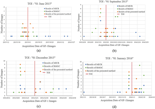
In terms of time span, the time spans obtained by the presented method all are the shortest in the four selected TOIs (red lines shown in Figure 14). Specifically, the time span for MICR results varies between 131 days, which is the shortest time span, and 389 days, which is the longest. For RMGC results, the shortest time span is 86 days, and the longest is 133 days. The presented method has a time span ranging from 53 days, which is the shortest, to 73 days, which is the longest. Compared to the MICR and RMGC methods, the proposed method reduces the averages by 76.1% and 38.7%, respectively. This is due to the effective use of cloudless areas in the images by the presented method, which shortens the time span required for full coverage image generation.

The experimental area is Hubei Province where many areas are cloudy areas. Moreover, partial GF-1 images from January 2015 to March 2016 are used in this paper due to the reason of data acquisition. It is foreseeable that if more satellites are available (such as the use of satellite constellations (Pontani and Teofilatto, 2022)) and more data can be obtained through a multi-satellite combination mode, the method proposed in this paper can further improve the timeliness.

3.4.2. Quality analysis of the results

Image selection results of MICR, RMGC, PTSM, and the presented method at selected TOIs are shown in Figure 15. Figure 15(a) shows that all the results of MICR still have visible clouds. Furthermore, the colors of the different images are significantly different, which seriously affects the subsequent application. This is because remote sensing images often cover large areas and few of them are entirely cloud-free. Since the RMGC only selects images based on a predetermined latitude and longitude range, it cannot actively avoid areas with cloud coverage. As a result, some images still contain varying degrees of cloud coverage (as shown in Figure 15(b)). Moreover, several results appear too many fragments. Figure 15(c) shows that some results of PTSM also contain areas with varying degrees of cloud coverage. Additionally, PTSM cannot answer how long the time span is required to be the shortest for the user to generate a full coverage composite image of the area at the TOI.

Figure 15. Experimental results of different methods at four TOIs. (a)-(d) From left to right are the results of MICR, RMGC, PTSM, and the presented method, respectively; A-D from top to bottom are the TOIs that are“01 June 2015”, “01 September 2015”, “01 December 2015”, and “01 January 2016”, respectively; I-Ⅴ are the marked numbers of selected regions.

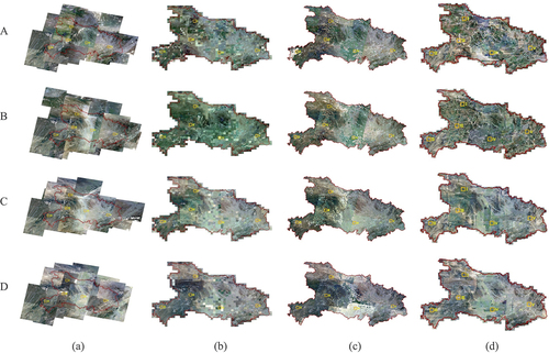
In contrast, there were hardly any clouds in the results of the presented method (as shown in Figure 15(d)). The presented method adopts a region quality grading algorithm that fully utilizes the cloudless coverage area in images to eliminate the influence of clouds. Thus, not only was the utilization rate of the image improved, but the quality of the composite image was also improved. The data are dynamically merged and extracted to construct the candidate dataset, which ensures the continuity of ground features in the final full coverage image.

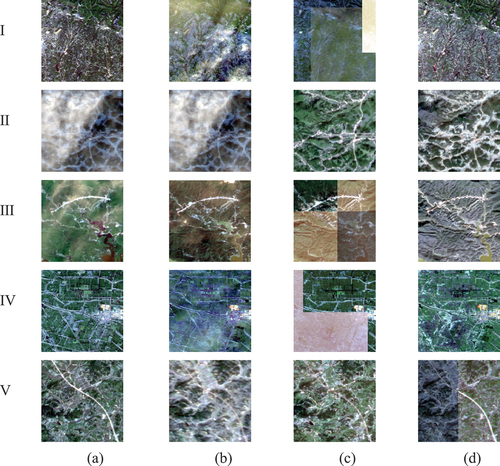
In the aspect of qualitative analysis, five regions (five marked orange rectangles by No. I-Ⅴ in Figure 15) from the results were randomly selected for visual comparison. Therefore, blocks were extracted from the results at four TOIs of four methods. Some examples of the blocks are shown in Figure 16. It can be observed that there are clouds in many blocks for the results of MICR, RMGC, and PTSM. For instance, in Figure 16(a), several blocks may not meet many application requirements due to cloud cover. In contrast, the results obtained from the presented method (Figure 16(d)) are more satisfactory.

Figure 16. Some examples of blocks obtained for visual comparison. (a)–(d) From left to right are the results of MICR, RMGC, PTSM, and the presented method, respectively; I–Ⅴ from top to bottom are five selected regions.

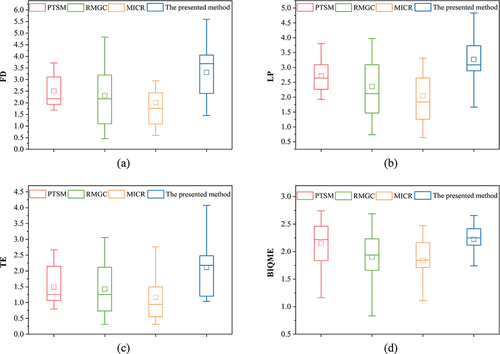
In the aspect of quantitative analysis, assessment indices are used to evaluate the quality of each selected region from the results at four TOIs for each method. At the same time, residual cloud amount is used to further evaluate the effectiveness for four methods. Figure 17 shows the box plots of assessment indices. The abscissa in the plot represents the method, and the ordinate represents the index value. The upper and lower limits of the box represent the first and third quartiles of the statistical data, respectively. The median of the assessment indices is presented as a line in the box, and the average of the assessment indices is presented as a square in the box. The higher the assessment indices are, the better the quality of the region is. Figure 17 shows the statistical distribution of the assessment indices on selected regions for four methods. As shown in Figure 17(a–c), the statistical results of the presented method in the assessment indices, including TE, FD, and LP, are higher than those of the other methods. As shown in Figure 17(d), the median and the third quartile of the statistical results of the presented method in the BIQME are also close to the highest values.

Figure 17. Box plots of the four assessment indices. (a)–(d) Are the statistical results of regional data under FD, LP, TE, and BIQME, respectively.

Clouds can obscure ground objects, and it is hard to obtain effective coverage of the land surface using cloudy images. Hence, to further evaluate the performance of the presented method, the residual cloud amounts of different methods at four TOIs are as shown in Figure 18. In Figure 18, yellow represents clouds. They were manually produced based on the results, and the lower the proportion of clouds, the better the quality of the results.

Figure 18. Cloud amounts of different methods at the different TOIs. (a)–(d) Represent the results of MICR, RMGC, PTSM, and the presented method, respectively; A–D represent the TOIs that are “01 June 2015”, “01 September 2015”, “01 December 2015”, and “ 01 January 2016”, respectively.

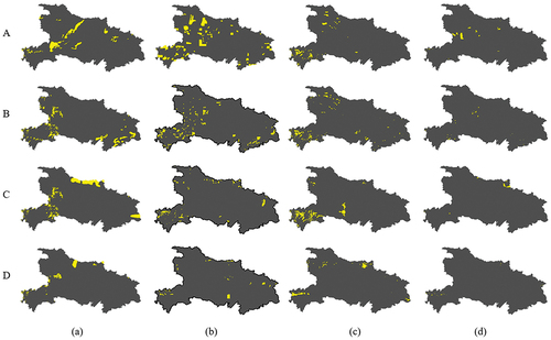
In terms of residual cloud amounts, the results obtained from the presented method are all lowest at four TOIs, which is also evident from the visualization results. Statistical results in Table 4 further confirm the effectiveness of the presented method. Specifically, the residual cloud amounts for the MICR, RMGC, PTSM, and proposed methods range from 5.28% to 1.91%, 7.51% to 1.01%, 2.84% to 1.38%, and 0.69% to 0.15%, respectively. Compared to the MICR, RMGC, and PTSM methods, the proposed method reduces the residual cloud amount by an average of 91.2%, 89.8%, and 83.4%, respectively. Consequently, the selection results obtained with the proposed method can be used for subsequent full coverage composite image generation.

Table 4. The proportion of clouds in the results of different methods at four TOIs (in pixels).

		Total pixels (60712)
TOI	Statistics	MICR	RMGC	PTSM	The presented method
1 June 2015	cloud	2562	4560	1244	419
	proportion of cloud (%)	4.22	7.51	2.05	0.69
1 September 2015	cloud	2719	2025	1223	132
	proportion of cloud (%)	4.49	3.34	2.01	0.22
1 December 2015	cloud	3206	969	1727	188
	proportion of cloud (%)	5.28	1.60	2.84	0.31
1 January 2016	cloud	1162	654	839	93
	proportion of cloud (%)	1.91	1.01	1.38	0.15

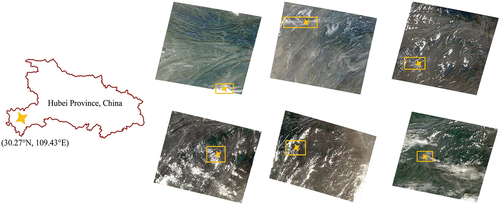
Although the presented method achieved the lowest residual cloud amount, it still cannot completely avoid cloud coverage. There are two possible reasons for this. One reason is that there are already clouds present in the same area of the existing data. For instance, as shown in Figure 19, all existing images in the area near the coordinates (30.27°N, 109.43°E) have cloud coverage. Another reason is that the accuracy of the region quality grading has not reached 100%, so there is a possibility that the quality of some regions has been graded incorrectly.

Figure 19. GF-1 images covering a same region.

4. Conclusions

In this paper, a new method of spatiotemporal imagery selection for full coverage image generation over a large area with HFA-Net based quality grading is proposed. A series of experiments were conducted on GF-1 satellite data covering Hubei Province. The results of the presented method, with a minimum imaging time span of only 53 days and residual cloud cover as low as 0.15%, were significantly better than those obtained using the comparative method. The experimental results demonstrate that the presented method can effectively utilize cloudless and high-quality regions in images, thereby improving the utilization rate of remote sensing data and shortening the time span of the image selection results. Furthermore, if more images are available, the timeliness of image selection results can be further improved, and the capacity of the earth observation system can be further exploited.

There is still room for the refinement of the image selection process for full coverage image generation. The result of the image selection is related to the result of quality grading, which means that the more accurate the quality grading result is, the better the selected result. Moreover, the data used in this paper are radiation-corrected data; however, there may still be radiometric inconsistencies due to factors such as view angle, atmospheric conditions, etc. In the next steps, further improvements will be considered to enhance the effectiveness of absolute radiometric correction (Claverie et al. 2018). For the remaining radiometric inconsistencies among different images, a relative radiometric correction method will be considered for processing (Roy et al. 2008; Vicente-Serrano et al. 2008). These issues will be addressed in the future work.

Acknowledgments

The authors would like to thank Supercomputing Center of Wuhan University for computational support and China Center for Resources Satellite Data and Application for providing experimental data.

Disclosure statement

No potential conflict of interest was reported by the author(s).

Data availability statement

The GF-1 data used can be queried and downloaded from the website of China Centre for Resources Satellite Data and Application (https://data.cresda.cn).

Additional information

Funding

This work is supported by the National Natural Science Foundation of China [grant numbers 41971422 and 42090010], and the Fundamental Research Funds for the Central Universities, China [grant number 2042022dx0001].

Notes on contributors

Jun Pan

Jun Pan received the B.Eng. degree in geographic information science and the M.Sc. and Ph.D. degrees in photogrammetry and remote sensing from Wuhan University, Wuhan, China, in 2002, 2005, and 2008, respectively. Since 2008, he has been a Professor with the State Key Laboratory of Information Engineering in Surveying, Mapping, and Remote Sensing, Wuhan University. His research interests are deep learning and intelligent mosaic of high-resolution remote sensing images.

Liangyu Chen

Liangyu Chen received the M.Sc. degree in surveying and mapping from China University of Geosciences, Wuhan, China, in 2019. He is currently pursuing the Ph.D. degree with the State Key Laboratory of Information Engineering in Surveying, Mapping, and Remote Sensing, Wuhan University. His research interests are cloud detection and the intelligent mosaic of high-resolution remote sensing images.

Qidi Shu

Qidi Shu received the M.Sc. degree in the State Key Laboratory of Information Engineering in Surveying, Mapping, and Remote Sensing, Wuhan University, in 2023. His research interest is change detection.

Qiang Zhao

Qiang Zhao received the M.Sc. degree in the State Key Laboratory of Information Engineering in Surveying, Mapping, and Remote Sensing, Wuhan University, in 2020. His research interest is data screening.

Jin Yang

Jin Yang received the M.Sc. degree in the State Key Laboratory of Information Engineering in Surveying, Mapping, and Remote Sensing, Wuhan University, in 2021. His research interest is deep learning.

Shuying Jin

Shuying Jin received the B.Eng. and Ph.D. degrees in photogrammetry and remote sensing from Wuhan University, in 1996 and 2007, respectively. Since 2009, she has been an associate professor in the State Key Laboratory of Information Engineering in Surveying, Mapping and Remote Sensing, Wuhan University. Her research interest is geometric processing of remote sensing images.

References

- Chen, B., L. Chen, B. Huang, R. Michishita, and B. Xu. 2018. “Dynamic Monitoring of the Poyang Lake Wetland by Integrating Landsat and MODIS Observations.” ISPRS Journal of Photogrammetry & Remote Sensing 139:75–87. https://doi.org/10.1016/j.isprsjprs.2018.02.021.
- Chen, L. Y., J. Pan, and Z. Zhang. 2023. “A Novel Cloud Detection Method Based on Segmentation Prior and Multiple Features for Sentinel-2 Images.” International Journal of Remote Sensing 44 (16): 5101–5120. https://doi.org/10.1080/01431161.2023.2243022.
- Christian, H., and F. Rottensteiner. 2020. “Deep Learning for Geometric and Semantic Tasks in Photogrammetry and Remote Sensing.” Geo-Spatial Information Science 23 (1): 10–19. https://doi.org/10.1080/10095020.2020.1718003.
- Chu, B., D. L. Jiang, and B. Cheng. 2014. “Large Scale Mosaic Using Parallel Computing for Remote Sensed Images.” Applied Mechanics & Materials 556-562:4746–4749. https://doi.org/10.4028/www.scientific.net/AMM.556-562.4746.
- Claverie, M., J. Ju, J. G. Masek, J. L. Dungan, E. F. Vermote, J. Roger, S. V. Skakun, and C. Justice. 2018. “The Harmonized Landsat and Sentinel-2 Surface Reflectance Data Set.” Remote Sensing of Environment 219:145–161. https://doi.org/10.1016/j.rse.2018.09.002.
- Eken, S., and A. Sayar. 2021. “A MapReduce-Based Distributed and Scalable Framework for Stitching of Satellite Mosaic Images.” Arabian Journal of Geosciences 14:1863. https://doi.org/10.1007/s12517-021-07500-w.
- Gao, H., L. Zhuang, M. Laurens, and Q. W. Kilian. 2017. “Densely Connected Convolutional Networks.” Paper presented at the 2017 IEEE Conference on Computer Vision and Pattern Recognition (CVPR), 2261–2269, Hawaii, July 21–26.
- Gao, S. H., M. M. Cheng, K. Zhao, X. Y. Zhang, M. H. Yang, and T. Philip. 2021. “Res2Net: A New Multi-Scale Backbone Architecture.” IEEE Transactions on Pattern Analysis & Machine Intelligence 43 (2): 652–662. https://doi.org/10.1109/TPAMI.2019.2938758.
- Geng, J., W. Gan, J. Xu, R. Yang, and S. Wang. 2020. “Support Vector Machine Regression (SVR)-Based Nonlinear Modeling of Radiometric Transforming Relation for the Coarse-Resolution Data-Referenced Relative Radiometric Normalization RRN.” Geo-Spatial Information Science 23 (3): 237–247. https://doi.org/10.1080/10095020.2020.1785958.
- Gu, K., D. Tao, J. F. Qiao, and W. S. Lin. 2018. “Learning a No-Reference Quality Assessment Model of Enhanced Images with Big Data.” IEEE Transactions on Neural Networks and Learning Systems 29 (4): 1301–1313. https://doi.org/10.1109/TNNLS.2017.2649101.
- He, K., X. Zhang, S. Ren, and J. Sun. 2016. “Deep Residual Learning for Image Recognition.” Paper presented at the 2016 IEEE Conference on Computer Vision and Pattern Recognition (CVPR), 770–778, Las Vegas, June 26–July 1.
- Hsu, C., and Y. Tsan. 2004. “Mosaics of Video Sequences with Moving Objects.” Signal Processing: Image Communication 19 (1): 81–98. https://doi.org/10.1016/j.image.2003.10.001.
- Hu, J., L. Shen, and G. Sun. 2018. “Squeeze-and-Excitation Networks.” Paper presented at the 2018 IEEE/CVF Conference on Computer Vision and Pattern Recognition, 7132–7141, Salt Lake City, June 18–22.
- King, M. D., S. Platnick, W. P. Menzel, and P. A. Hubanks. 2013. “Spatial and Temporal Distribution of Clouds Observed by MODIS Onboard the Terra and Aqua Satellites.” IEEE Transactions on Geoscience & Remote Sensing 51 (7): 3826–3852. https://doi.org/10.1109/TGRS.2012.2227333.
- Lai, J., X. Luo, T. Yu, and P. Jia. 2013. “Remote Sensing Data Organization Model Based on Cloud Computing.” Computer Science 40 (7): 80–83. http://www.jsjkx.com/CN/Y2013/V40/I7/80.
- Li, D., M. Wang, and J. Jiang. 2021. “China’s High-Resolution Optical Remote Sensing Satellites and Their Mapping Applications.” Geo-Spatial Information Science 24 (1): 85–94. https://doi.org/10.1080/10095020.2020.1838957.
- Li, F., S. You, H. Wei, E. Wei, and L. Chen. 2017. “An Optimal Dataset Screening Model for Remote-Sensing Imagery Regional Coverage.” Radio Engineering 47 (10): 45–48. https://doi.org/10.3969/j.issn.1003-3106.2017.10.10.
- Li, Z., X. Zhao, C. Zhao, M. Tang, and J. Wang. 2022. “Transfering Low-Frequency Features for Domain Adaptation.” Paper presented at the 2022 IEEE International Conference on Multimedia and Expo (ICME), 1–6, Taipei, July 18–22.
- Liu, S., H. Su, G. Cao, S. Wang, and Q. Guan. 2019. “Learning from Data: A Post Classification Method for Annual Land Cover Analysis in Urban Areas.” Isprs Journal of Photogrammetry & Remote Sensing 154:202–215. https://doi.org/10.1016/j.isprsjprs.2019.06.006.
- Liu, T., P. Li, L. Zhang, and X. Chen. 2008. “Multi-Spectral Remote Sensing Image Retrieval Based on Semantic Extraction.” Paper presented at the International Conference on Earth Observation Data Processing and Analysis (ICEODPA), 267–274, Wuhan, December 28–30.
- Liu, Z., Y. Lin, Y. Cao, H. Hu, Y. Wei, Z. Zhang, S. Lin, and B. Guo. 2021. “Swin Transformer: Hierarchical Vision Transformer Using Shifted Windows.” arXiv: 2103.14030. https://doi.org/10.48550/arXiv.2103.14030.
- Luo, Y., Y. Zhang, J. Yan, and W. Liu. 2021. “Generalizing Face Forgery Detection with High-Frequency Features.” Paper presented at the 2021 IEEE/CVF conference on computer vision and pattern recognition, 16317–16326, Online, June 19–25.
- Mansour, A. G., M. S. Eid, and E. E. Elbeltagi. 2022. “Construction Facilities Location Selection for Urban Linear Infrastructure Maintenance Projects Using Uniform Cost Search Method.” Soft Computing 26:1403–1415. https://doi.org/10.1007/s00500-021-06408-7.
- Miao, L., X. Li, L. Zhou, Q. Wen, Z. Jin, Z. Xiong, G. Jin, and L. Hu. 2010. “Fast Approach for Querying Coverage of Multi-Source RS Data and Its Realization Based on ENVI/IDL.” Remote Sensing Technology and Application 25 (4): 502–509. https://doi.org/10.11873/j.issn.1004-0323.2010.4.502.
- Michele, M., F. Dominique, R. Felix, A. Clement, and K. Anja. 2019. “Near Real-Time Vegetation Anomaly Detection with MODIS NDVI: Timeliness Vs. Accuracy and Effect of Anomaly Computation Options.” Remote Sensing of Environment 221:508–521. https://doi.org/10.1016/j.rse.2018.11.041.
- Montavon, G., W. Samek, and K. R. Müller. 2018. “Methods for Interpreting and Understanding Deep Neural Networks.” Digital Signal Processing 73:1–15. https://doi.org/10.1016/j.dsp.2017.10.011.
- NASA’s GeoCover 2000 Landsat Product Promotes Geo-Commerce Globally. 2016. Accessed January 1, 2023. https://landsat.gsfc.nasa.gov/.
- Pontani, M., and P. Teofilatto. 2022. “Deployment Strategies of a Satellite Constellation for Polar Ice Monitoring.” Acta Astronautica 193:346–356. https://doi.org/10.1016/j.actaastro.2021.12.008.
- Prins, A. J., and A. V. Niekerk. 2021. “Crop Type Mapping Using LiDar, Sentinel-2 and Aerial Imagery with Machine Learning Algorithms.” Geo-Spatial Information Science 24 (2): 215–227. https://doi.org/10.1080/10095020.2020.1782776.
- Rao, H. 2019. “A Method of Retrieving Remote Sensing Image Data with Grid Compensation.” China Computer & Communication 6:136–141.
- Roy, D. P., J. Ju, K. Kline, P. L. Scaramuzza, V. Kovalskyy, M. Hansen, T. R. Loveland, E. Vermote, and C. Zhang. 2010. “Web-Enabled Landsat Data (WELD): Landsat ETM+ Composited Mosaics of the Conterminous United States.” Remote Sensing of Environment 114 (1): 35–49. https://doi.org/10.1016/j.rse.2009.08.011.
- Roy, D. P., J. Ju, P. Lewis, C. Schaaf, F. Gao, M. Hansen, and E. Lindquist. 2008. “Multi-Temporal MODIS–Landsat Data Fusion for Relative Radiometric Normalization, Gap Filling, and Prediction of Landsat Data.” Remote Sensing of Environment 112 (6): 3112–3130. https://doi.org/10.1016/j.rse.2008.03.009.
- Roy, D. P., H. K. Zhang, J. Ju, J. L. Gomez-Dans, P. E. Lewis, C. B. Schaaf, Q. Sun, J. Li, H. Huang, and V. Kovalskyy. 2016. “A General Method to Normalize Landsat Reflectance Data to Nadir BRDF Adjusted Reflectance.” Remote Sensing of Environment 176:255–271. https://doi.org/10.1016/j.rse.2016.01.023.
- Sahoo, A. K., G. Kumar, G. Mishra, and R. Misra. 2015. “A New Approach for Parallel Region Growing Algorithm in Image Segmentation Using MATLAB on GPU Architecture.” Paper presented at the 2015 IEEE International Conference on Computer Graphics, Vision and Information Security (CGVIS), 279–283, Bhubaneshwar, November 2–3.
- Simonyan, K., and A. Zisserman. 2014. “Very Deep Convolutional Networks for Large-Scale Image Recognition.” arXiv preprint arXiv: 1409.1556. https://doi.org/10.48550/arXiv.1409.1556.
- Tariq, A., J. Yan, A. S. Gagnon, M. R. Khan, and F. Mumtaz. 2022. “Mapping of Cropland, Cropping Patterns and Crop Types by Combining Optical Remote Sensing Images with Decision Tree Classifier and Random Forest.” Geo-Spatial Information Science 1–19. https://doi.org/10.1080/10095020.2022.2100287.
- Theodomir, M., H. Sebastian, H. Jan, and B. Yifang. 2022. “Monitoring Urbanization and Environmental Impact in Kigali, Rwanda Using Sentinel-2 MSI Data and Ecosystem Service Bundles.” International Journal of Applied Earth Observation and Geoinformation 109 (102775). https://doi.org/10.1016/j.jag.2022.102775.
- Venetsanos, A. G., J. G. Bartzis, J. Würtz, and D. D. Papailiou. 2003. “DISPLAY-2: A Two-Dimensional Shallow Layer Model for Dense Gas Dispersion Including Complex Features.” Journal of Hazardous Materials 99 (2): 111–144. https://doi.org/10.1016/S0304-3894(03)00011-6.
- Vicente-Serrano, S. M., F. Pérez-Cabello, and T. Lasanta. 2008. “Assessment of Radiometric Correction Techniques in Analyzing Vegetation Variability and Change Using Time Series of Landsat Images.” Remote Sensing of Environment 112 (10): 3916–3934. https://doi.org/10.1016/j.rse.2008.06.011.
- Wang, Y., M. Wang, Y. Zhu, and X. Long. 2022. “Low Frequency Error Analysis and Calibration for Multiple Star Sensors System of GaoFen7 Satellite.” Geo-Spatial Information Science 1–13. https://doi.org/10.1080/10095020.2022.2100284.
- Wexler, Y., E. Shechtman, and M. Irani. 2007. “Space-Time Completion of Video.” IEEE Transactions on Pattern Analysis & Machine Intelligence 29 (3): 463–476. https://doi.org/10.1109/TPAMI.2007.60.
- Xie, S., R. Girshick, P. Dollar, Z. Tu, and K. He. 2017. “Aggregated Residual Transformations for Deep Neural Networks.” Paper presented at the 2017 IEEE Conference on Computer Vision and Pattern Recognition (CVPR), 5987–5995. Hawaii, July 21–26.
- Xu, Y., K. Li, J. Hu, and K. Li. 2014. “A Genetic Algorithm for Task Scheduling on Heterogeneous Computing Systems Using Multiple Priority Queues.” Information Sciences 270:255–287. https://doi.org/10.1016/j.ins.2014.02.122.
- Xue, T., M. Diao, J. Li, and S. Zou. 2013. “Approach to Storing, Retrieving and Accessing Mass Spatial Data in Resources and Environments Remote Sensing.” Remote Sensing for Land & Resources 25 (2): 168–173. https://doi.org/10.6046/gtzyyg.2013.02.28.
- Yan, X., S. Liu, W. Liu, and Q. Dai. 2022. “An Improved Coverage-Oriented Retrieval Algorithm for Large-Area Remote Sensing Data.” International Journal of Digital Earth 15 (1): 606–625. https://doi.org/10.1080/17538947.2022.2030816.
- Yuan, W., X. Yuan, Y. Cai, and R. Shibasaki. 2023. “Fully Automatic DOM Generation Method Based on Optical Flow Field Dense Image Matching.” Geo-Spatial Information Science 26 (2): 242–256. https://doi.org/10.1080/10095020.2022.2159886.
- Zagoruyko, S., and N. Komodakis. 2016. “Wide Residual Networks.” arXiv preprint arXiv: 1605.07146. https://doi.org/10.48550/arXiv.1605.07146.
- Zhang, W., L. Jiao, F. Liu, J. Liu, and Z. Cui. 2022. “LHNet: Laplacian Convolutional Block for Remote Sensing Image Scene Classification.” In IEEE Transactions on Geoscience and Remote Sensing, 1–13. https://doi.org/10.1109/TGRS.2022.3192321.
- Zhang, Z., Q. Yuan, Z. Li, F. Sun, and L. Zhang. 2021. “Combined Deep Prior with Low-Rank Tensor SVD for Thick Cloud Removal in Multitemporal Images.” Isprs Journal of Photogrammetry & Remote Sensing 177:161–173. https://doi.org/10.1016/j.isprsjprs.2021.04.021.
- Zuo, X., M. Xiong, X. Huang, W. Zang, and D. Shang. 2018. “A Full Coverage Retrieval Mode and Method for Remote Sensing Tile Data.” Journal of Henan University (Natural Science) 48 (3): 299–308. https://doi.org/10.15991/j.cnki.411100.2018.03.006.