Modeling information flow from multispectral remote sensing images to land use and land cover maps for understanding classification mechanism

ABSTRACT

Information on Land Use and Land Cover Map (LULCM) is essential for environment and socioeconomic applications. Such maps are generally derived from Multispectral Remote Sensing Images (MRSI) via classification. The classification process can be described as information flow from images to maps through a trained classifier. Characterizing the information flow is essential for understanding the classification mechanism, providing solutions that address such theoretical issues as “what is the maximum number of classes that can be classified from a given MRSI?” and “how much information gain can be obtained?” Consequently, two interesting questions naturally arise, i.e. (i) How can we characterize the information flow? and (ii) What is the mathematical form of the information flow? To answer these two questions, this study first hypothesizes that thermodynamic entropy is the appropriate measure of information for both MRSI and LULCM. This hypothesis is then supported by kinetic-theory-based experiments. Thereafter, upon such an entropy, a generalized Jarzynski equation is formulated to mathematically model the information flow, which contains such parameters as thermodynamic entropy of MRSI, thermodynamic entropy of LULCM, weighted F1-score (classification accuracy), and total number of classes. This generalized Jarzynski equation has been successfully validated by hypothesis-driven experiments where 694 Sentinel-2 images are classified into 10 classes by four classical classifiers. This study provides a way for linking thermodynamic laws and concepts to the characterization and understanding of information flow in land cover classification, opening a new door for constructing domain knowledge.

KEYWORDS:

• Multispectral Remote Sensing Image (MRSI)
• Land Use and Land Cover Map (LULCM)
• classification mechanism
• information flow
• statistical thermodynamics
• the law of energy conservation

View correction statement:

Correction

1. Introduction

Land Use and Land Cover Map (LULCM) is of importance for various environmental and socioeconomic applications such as forest management (Quan et al. 2023; White et al. 2022), urban planning (Zhong et al. 2023; Zhou et al. 2023), environmental management (Kim, Jeong, and Kim 2021; Wang et al. 2022), and agriculture monitoring (Benami et al. 2021; Weiss, Jacob, and Duveiller 2020). The generation of such maps is normally achieved by classifying MRSI that concern geographical objects and/or phenomena at various scales (spatial, spectral, and temporal) and record energy with the reflectance measurements of objects (Chen et al. 2015). MRSI classification is a complicated process that involves many factors (Lu and Weng 2007; Prudente et al. 2022; Long and Singh 2013), including the complexity of landscape in the study area, selection of training samples, selection of images, image preprocessing, feature extraction, selection and design of classifiers, post-classification, and accuracy assessment. Despite these complicated factors, MRSI classification has been captivating attention from researchers and practitioners, particularly along with the emergence of multi-modal remote sensing data (e.g. Unmanned Aerial Vehicle (UAV)) and advanced classification approaches ranging from traditional ones (e.g. Support Vector Machine (SVM) and Random Forest (RF)) to deep learning-based techniques (e.g. Convolutional Neural Networks (CNN)).

From the side of information, efforts on promoting Multispectral Remote Sensing Images (MRSI) classification falls into two categories: (i) information extraction and (ii) information flow modeling. For the former, researchers are mainly concerned with how an image can be accurately classified and/or segmented for given classes. Great efforts have been focused on extraction of features, design and optimization of classifiers (Ma et al. 2019; Marinoni, Iannelli, and Gamba 2017; Tuia et al. 2011; Zhong, Ma, and Zhang 2014; Li et al. 2022). As a result, spatial-temporal information of geographical objects and phenomena is then extracted from MRSI with accuracy via valid operators (e.g. convolution, clustering, pooling, and scaling) and their effective assemble and combinations. For the latter, a holistic understanding can help quantify the variation of causality in unsupervised and/or supervised classification. It is also useful for providing solutions to some theoretical issues in MRSI processing chain, e.g., (i) determination of the maximum number of classes that can be classified for a given MRSI, (ii) characterization of the amount of information essential to users that can be acquired from MRSI, and (iii) evaluation of the performance of a classifier on the new data without ground truth. However, the efforts on the information flow modeling are relatively little. Knopfli (1983) made one of the first attempts, considering that MRSI classification is a kind of process that information is transmitted from map makers to users, which can be explained by Shannon’s information theory (Shannon 1948; Shannon and Weaver 1972). Nonetheless, such an effort failed short of finding a practical and holistic solution for directly understanding information flow from MRSI to LULCM, because Shannon entropy is only capable of describing the spectral configuration of images/maps but not their spatial configuration (Cheng and Li 2021a, 2021b). Fortunately, a feasible method for computing configurational entropy has been developed (Gao, Zhang, and Li 2017) and thus Knopfli’s failed effort can be continued now. That is, this study aims to mathematically model the information flow from MRSI to LULCM with thermodynamic entropy and the law of energy conservation.

The remaining of this paper is organized as follows. After this introduction, a line of thought is first introduced. Second, the appropriateness of thermodynamic entropy for measuring the information content of MRSI and LULCM is discussed. Third, the Jarzynski equation is generalized to model the information flow from MRSI to LULCM. Fourth, the experimental validation of such a model is reported. Finally, a discussion and some conclusions are made.

2. Information flow from MSRI to LULCM: a line of thought

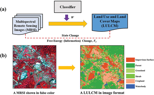
This study considers the state change from MRSI to LULCM with statistical thermodynamics. Theoretically speaking, MRSI classification can be considered as a thermodynamic process that involves the information flow and loss.

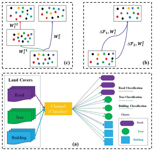
Figure 1(a) shows that MRSI classification via a channel (a classifier) is represented as a kind of process where the same land covers (microstates) distributed in different image regions can be classified into various classes (macrostates) due to different paths. The state change from microstates to a macrostate is accompanied with the information flow. Such a change is similar to two examples of thermodynamic processes that involve along with an ensemble of trajectories and free energy change. Figure 1(b) demonstrates that a thermodynamic ensemble is changed to the same final state on different paths where ∆${\mathcal{F}}_1$ and ∆${\mathcal{F}}_2$ represent the energy (information) change, $W_1$ and $W_2$ denote the thermodynamic work acting on the system, and $\mathrm{\Delta }{\mathcal{F}}_1$ is equal to $\mathrm{\Delta }{\mathcal{F}}_2$, though $W_1$ is not the same as $W_2$ (Maldague 2004). Figure 1(c) illustrates the behavior changes of a thermodynamic system with the same work ($W_t^2$= $W_t^{11}$+$W_t^{12}$) but different energy (information) change derived by different paths (Parrondo, Horowitz, and Sagawa 2015).

Figure 1. Schematic diagram of a linkage between MRSI classification and thermodynamics processes.

None of astounding models, however, have been developed to characterize the information flow toward MRSI classification, though central organizing theories or principles (e.g. the laws of thermodynamics, fluctuation theorems) are available. Note that the first law of thermodynamics (also known as the law of energy conservation) states that the total energy of a thermodynamic system is constant, though it can be changed from one form to others (Joule 1850; Wheeler 1999), providing us with well-established rules and concepts to characterize the information flow.

Based on the first law of thermodynamics, a powerful quantitative measure that characterizes a macrostate and its microstates should be needed to model the information flow. As information and energy are linearly interconvertible (Stonier 1996; Szilard 1929; Toyabe et al. 2010), the authors claim that thermodynamic entropy (Boltzmann 1872; Gressman and Strain 2010) should be considered here. As a quantitative measure that characterizes the “disorder” of a thermodynamic system from a given macrostate to multiple microstates, thermodynamic entropy captures information of both composition and configuration. However, outside of thermodynamics, one of the two key concepts—macrostate— is difficult to define and the other concept—number of microstates—is not easy to quantify. Fortunately, this problem has been solved, leading to a set of computation methods for numerical and nominal raster data (Cushman 2016; Gao and Li 2019; Gao, Zhang, and Li 2017), which will be introduced in Section 3.2.

With such development, it is now believed by the authors that we are able to carry out an investigation into the information flow from MRSI to LULCM and then establish some theoretical models for characterizing it.

3. Thermodynamic entropy for characterizing the information flow from MRSI to LULCM

3.1 Thermodynamic ensembles and configurations of MRSI and LULCM: a linkage

In physics, thermodynamics is commonly considered as the discipline concerned with energy transformation and the changes in the states of matter (Guggenheim 1967). As one of branch of thermodynamics, statistical thermodynamics aims to develop methods for characterizing the effect and phenomena of heat and work upon a system, e.g. the motion of molecules and corresponding configurations (Fowler and Guggenheim 1949).

Note that the analogy between images and thermodynamic ensembles has already been made. Indeed, some researchers have found thermodynamic features of MRSI (Geman and Geman 1984; Naveh 1987), for which the entropy per cell is approximated as a function of energy. Furthermore, Stephens et al. (2013) estimated entropy for image patches of different sizes and found that the thermodynamic entropy was highly consistent with the thermodynamic limit (logarithmic). In their study, thermodynamic features can be seen that the thermodynamic entropy fluctuates around the maximum theoretical value, which is associated with the most probable state (i.e. a perfectly random pattern). Nevertheless, such distribution varies among differently sized patches (for more details, readers can refer to Stephens et al. 2013). This also indicates that the image patch size should be modeled in the estimation of the thermodynamic entropy of MRSI. To this end, Section 3.2 will introduce the thermodynamic entropies of MRSI and LULCM followed by Section 3.3 that illustrates the verification of their thermodynamic features.

3.2 Thermodynamic entropy for information content of MRSI and LULCM

3.2.1 Thermodynamic entropy of MRSI

As an essential concept in statistical thermodynamics, the thermodynamic entropy (also called Boltzmann entropy) is defined as follows:

(1) $\begin{array}{c}S=k_b\times log{W}_b\end{array}$(1)

where $k_b$ is Boltzmann constant (1.38 × ${10}^{23}$ J/K), and $W_b$ represents the number of all possible microstates for a given macrostate (Boltzmann 1872).

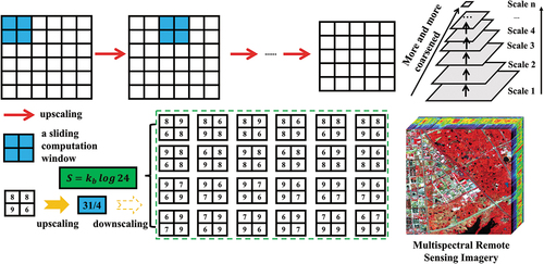
Gao et al. (2017) made an important advance in proposing a conceptualization and computational method for thermodynamic entropy of numerical raster data. To simulate thermodynamic cases as far as possible, a 2 × 2 sliding window is taken as the minimum computation unit (i.e. the minimum thermodynamic ensemble) wherein four cells are considered as gas molecules. The macrostate is then defined as the “upscaling” result (the mean of cell values) upon the i-th 2 × 2 patch; the corresponding microstates, $W_b^i$, are all possible permutation patterns of decomposition results. Furthermore, the thermodynamic entropy ($S_R$) for a 2 × 2 image is defined by

(2) $\begin{array}{c}{S}_R=\sum _{i=1}^M{W}_b^i\end{array}$(2)

where M denotes the total number of 2 × 2 patches.

Figure 2 shows a case for calculating thermodynamic entropy. By using the “upscaling”, the entropy of an image can be quantified as the sum of the $S_R$ across all scales.

Figure 2. Schematic diagram of calculating thermodynamic entropy of MRSI by the resampling-based method where $k_b$ is set to be 1 as suggested by Cushman (2016).

Given the thermodynamic entropy of a composite thermodynamic ensemble is additive over the constituent sub-ensembles (Landauer 1991; Toyabe et al. 2010), the relative thermodynamic entropy of MRSI, is then defined as follows:

(3) $\begin{array}{c}{S}_{MRSI}=\sum _{\alpha }{S}_R\left(N_1^{\alpha },N_2^{\alpha },\dots ,N_r^{\alpha }\right)\end{array}$(3)

where $\alpha$ represents the $\alpha$-th band, $N_r^{\alpha }$ represent all pixels within the r-th sub-ensemble (i.e. 2 × 2 image patch). Further discussion of the appropriateness of this equation is given in Section 3.4.

3.2.2 Thermodynamic entropy of LULCM

The quantitative measures for a thermodynamic system in the research of statistical thermodynamics should remain consistent as far as possible (Toyabe et al. 2010). Therefore, for LULCM, the aforementioned method of calculating thermodynamic entropy of MRSI has been generalized by Gao and Li (2019). Concretely, by using Equation (1)(1) $\begin{array}{c}S=k_b\times log{W}_b\end{array}$(1) , the thermodynamic entropy of a LULCM, $S_{LULCM}$, can be computed by

(4) $\begin{array}{c}{S}_{LULCM}=\sum _{i=1}^{I}log{W}_b^i\end{array}$(4)

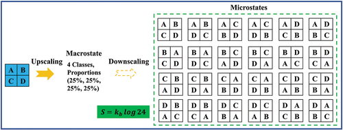
where $W_b^i$ is the number of microstates for i-th patch are all possible permutation patterns derived from the macrostate (i.e. the percentages and the total number of classes), as illustrated in Figure 3.

Figure 3. A case of calculating thermodynamic entropy of a LULCM. A, B, C and D represent four various land cover classes.

The thermodynamic entropy calculated by Gao et al. (2017) and Gao and Li (2019) are called “relative thermodynamic entropy”. One may note that the multiscale information of images is more appealing. To this end, they defined “absolute thermodynamic entropy” of images and maps as the sum of relative thermodynamic entropies computed from the original level to a single cell by using a 2 × 2 sliding window.

Indeed, as mentioned in Section 3.1, the patch size is an essential factor for estimating information content of images and maps. Furthermore, the total number of patches for an image or a map is determined by the way of multiscale representation, which is varied across different rules. Thus, to examine the reliability of the computation methods based on a 2 × 2 sliding window, we should use different multiscale representation rules to help compute the absolute thermodynamic entropy.

3.3 Verification of thermodynamic entropy for characterizing thermodynamic features

Before introducing the experiments of verifying thermodynamic entropy, two essential points should be critically considered. The first one is that thermodynamic entropy should demonstrate the consistency, i.e. thermodynamic entropy values of MRSI and LULCM exhibit a sideway trend during such a process from the “non-equilibrium” state (the most homogenous one) to the “equilibrium” state (the most heterogenous one). The second one is that the consistency should be invariant in various multi-scale representations, indicating absolute thermodynamic entropy (i.e. the sum of relative thermodynamic entropy across all spatial scales) should also show a sideway trend.

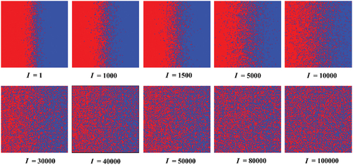
This study carried out experiments for examining the appropriateness of thermodynamic entropy according to Gao and Li (2019). According to the second law of thermodynamics, a closed thermodynamic ensemble spontaneously evolves from the “non-equilibrium” state to the “equilibrium” state. To this end, this study generated 100, 000 simulated cases with a kinetic theory-based approach (Gao and Li 2019), of which 10 cases can be seen in Figure 4 where the values of red and blue pixels are 2 and 4, respectively. Intuitively, the configuration of a simulated case is becoming increasingly random with the increase of iterations, indicating the increase in thermodynamic entropy value.

Figure 4. The configuration of landscape gradients is changed with the increasing iterations of mixing (I).

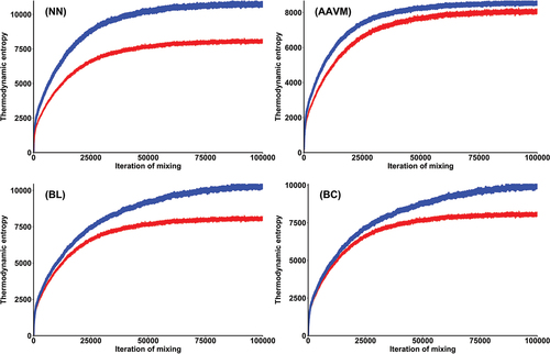
The key to inferring spatial information across spatial scales is the measurement of dominant spatial features, patterns, and processes of a variable (Wang, Gertner, and Anderson 2004). Therefore, four typical upscaling techniques are employed, i.e. Nearest Neighbor (NN), Arithmetic Average Variability Weighted (AAVW) (Wang, Gertner, and Anderson 2004), Bilinear (BL), Bicubic (BC), to generate a series of cases from fine to coarse spatial resolutions.

Figure 5 demonstrates the variation of thermodynamic entropy by different upscaling methods, indicating consistency with the second law of thermodynamics (Carnot 1943) as both the relative and multi-scale thermodynamic entropy increase along with the iterations and remain relatively stable after reaching the maximum value. In the “equilibrium” state (i.e. iteration of mixing ranged from 80,000 to 100,000), the values of thermodynamic entropy fluctuate around the maximum one. Note that various upscaling methods have different performances in estimating the multiscale information of images.

Figure 5. Variation of the relative and absolute thermodynamic entropy of simulated images computed by different upscaling methods with the 100,000 iterations of mixing. “Blue” denotes the absolute thermodynamic entropy. “Red” represents the relative thermodynamic entropy.

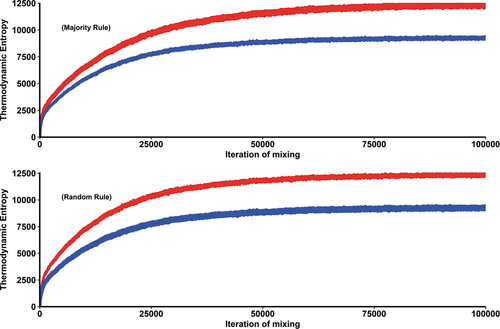
Regarding the multiscale representation of maps, two widely used rules, i.e. majority and random (He, Ventura, and Mladenoff 2002), are utilized. It is worth noting that Figure 6 demonstrates that the behavior of thermodynamic entropy is the same as Figure 5.

Figure 6. Variation of the relative and absolute thermodynamic entropy for simulated LULCM derived from different upscaling methods with the iteration of mixing. “Red” denotes $S_{LULCM}^M$, the multi-scale thermodynamic entropy. “Blue” represents $S_{LULCM}$, the relative thermodynamic entropy.

The experimental results show that the 2 × 2 sliding-window-based computation methods for thermodynamic entropy are reliable for describing the thermodynamic features, providing the operational quantitative measurement of information of MRSI and LULCM. It is thus reliable to employ thermodynamic entropy as a tool to model the information flow from MRSI to LULCM. Note that the use of relative or absolute thermodynamic entropy is subject to practical applications. Considering the hierarchical representation of raster data, absolute thermodynamic entropy quantifies multiscale spatial information (Gao, Zhang, and Li 2017), providing tools for investigating information across multiple spatial scales. This study investigates the information of MRSI and LULCM at original spatial scale and thus relative thermodynamic entropy is considered as the mathematic measure in the following sections.

3.4 Inferring information of MRSI via thermodynamic entropy

In thermodynamics modeling, connections between thermodynamic ensembles are critically considered (Chandler 1987; Toyabe et al. 2010). In turn, one may note that the estimation of information of MRSI by Equation (3)(3) $\begin{array}{c}{S}_{MRSI}=\sum _{\alpha }{S}_R\left(N_1^{\alpha },N_2^{\alpha },\dots ,N_r^{\alpha }\right)\end{array}$(3) ignores the spectral correlation. Therefore, the relative thermodynamic entropy of MRSI can be further estimated with two ways after decorrelation. One is the mean of relative thermodynamic entropy of MRSI with G bands, i.e. $S_{MMRSI}$, as follows:

(5) $\begin{array}{c}{S}_{MMSRI}=\sum _{\mathrm{g}=1}^G\frac{S_{MRSI}^g}{G}\end{array}$(5)

The other one is the weighted relative thermodynamic entropy of MRSI, i.e.

(6) $\begin{array}{c}{S}_{WMRSI}=\sum _{g=1}^G{W}_g\times S_{MRSI}^g\end{array}$(6)

where $S_{MRSI}^g$ denotes the relative thermodynamic entropy of the g^th component and ${\mathrm{W}}_g$ represents contribution ratio.

In this study, unless otherwise stated, Equation (3)(3) $\begin{array}{c}{S}_{MRSI}=\sum _{\alpha }{S}_R\left(N_1^{\alpha },N_2^{\alpha },\dots ,N_r^{\alpha }\right)\end{array}$(3) is mainly employed to quantify the information of MRSI, whereas the use of Equations (5)(5) $\begin{array}{c}{S}_{MMSRI}=\sum _{\mathrm{g}=1}^G\frac{S_{MRSI}^g}{G}\end{array}$(5) and (6(6) $\begin{array}{c}{S}_{WMRSI}=\sum _{g=1}^G{W}_g\times S_{MRSI}^g\end{array}$(6) ) are also discussed in the following sections. Two classical decorrelation techniques are employed, i.e. Principal Component Analysis (PCA) (Fukunaga 1990) and Independent Component Analysis (ICA) (Hyvärinen, Karhunen, and Oja 2001; Jutten and Herault 1991). Further discussion of the effect of decorrelation is given in Section 6.

4. A generalized Jarzynski equation for information flow from MRSI to LULCM

4.1 Jarzynski equation for the first law of thermodynamics

According to the first law of thermodynamics, the free energy difference $\mathrm{\Delta }\mathcal{F}$ between two states A and B can be expressed with

(7) $\begin{array}{c}\mathrm{\Delta }\mathcal{F}\le W_t\end{array}$(7)

where the $W_t$ is thermodynamic work acting on the thermodynamic system.

The equality holds for a quasi-static process case. Such a case means that all intermediates are in thermodynamic equilibrium in the process from state A to state B. Such a process can be described by the Jarzynski equation (Jarzynski 1997), which states:

(8) $\begin{array}{c}{e}^{-\frac{\mathrm{\Delta }\mathcal{F}}{k_{b}T}}=\stackrel{‾}{e^{-\frac{W_t}{k_{b}T}}}\end{array}$(8)

$k_b$ and T hold the same meanings as in Equation (1)(1) $\begin{array}{c}S=k_b\times log{W}_b\end{array}$(1) , $W_t$ depends upon the specific initial microstates of the system, and $\stackrel{‾}{}$ means the average value. Note that the Jarzynski equation is always valid no matter how the thermodynamic process happens. By using Jensen’s inequality (Chandler 1987) in statistical mechanics, Equation (8)(8) $\begin{array}{c}{e}^{-\frac{\mathrm{\Delta }\mathcal{F}}{k_{b}T}}=\stackrel{‾}{e^{-\frac{W_t}{k_{b}T}}}\end{array}$(8) can be rewritten as

(9) $\begin{array}{c}\mathrm{\Delta }\mathcal{F}\le \overline{W_t}\end{array}$(9)

4.2 The transformation of MRSI into LULCM: two thermodynamics-based hypotheses

From the perspective of statistical thermodynamics, the state change of raster data can be considered an irreversible process as shown in Figure 7. In this study, two symbols, i.e. W and $F_c$, are employed to distinguish them from the $W_t$ and $\mathrm{\Delta }\mathcal{F}$ mentioned in Equation (9)(9) $\begin{array}{c}\mathrm{\Delta }\mathcal{F}\le \overline{W_t}\end{array}$(9) used in physics. As one can imagine, the work by the classifiers enables the MRSI to be converted into LULCM, along with the energy flow.

Figure 7. The schematic representation of transforming MRSI into LULCM as a thermodynamic process. (a). MRSI classification where W means the work acting upon MRSI by a classifier. (b) Raster data type is changed from numerical to nominal. The same land cover and land use distributed in different image parts is grouped into one class in the raster map.

Therefore, two hypotheses are made as follows:

1. The information flow from MRSI to LULCM can be described by thermodynamic entropy. The relationship between $S_{MRSI}$ and $S_{LULCM}$ are nonlinear, as shown in Figure 8(a).

   Figure 8. Schematic representation of two hypotheses raised in this study. $S_{MRSI}$ in (a) quantitively measures a MRSI from homogeneous to heterogeneous. $S_{LULCM}$ denotes the thermodynamic entropy value of maps derived from a MRSI.

   

2. The information flow is consistent with the law of energy conservation. The range of $F_c$ is the same as that of W, as illustrated in Figure 8(b). Moreover, a linear model can be built to characterize the information flow.

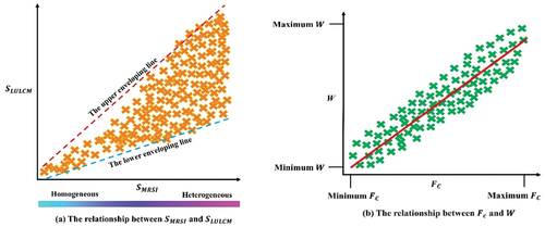
The first hypothesis can be easily illustrated by scatter plots. As mentioned in Section 3.3, the thermodynamic entropy of MRSI and LULCM is both thermodynamically consistent, it thus can be expected that the range between upper and lower enveloping lines of the $S_{LULCM}$ “predicted” by $S_{MRSI}$ will be increasingly large. Indeed, it is easy to be understood with two points. That is, (i) for a given classification scheme, LULCM derived from MRSI can be varied, which depends on the complexity of landscape in the study area and the classification performance of classifiers and (ii) The maximum theoretical thermodynamic entropy value exists for both LULCM and MRSI, whereas $S_{LULCM}$ and $S_{MRSI}$ values fluctuate around those theoretical ones, as illustrated in Figures 5 and 6.

To test the second hypothesis, we need to define the $F_c$ and W with $S_{MRSI}$ and $S_{LULCM}$ as well as other metrics for quantifying the working performance of a classifier, which will be introduced in Section 4.3.

4.3 Thermodynamic-entropy-based generalization of Jarzynski equation

Regarding the transformation of MRSI into LULCM, Equation (9)(9) $\begin{array}{c}\mathrm{\Delta }\mathcal{F}\le \overline{W_t}\end{array}$(9) can be generalized in accordance with Figure 7 as follows:

(10) $\begin{array}{c}ln{F}_c\le lnW\end{array}$(10)

where the logarithmic function is designed for quantifying information content as suggested by Toyabe et al. (2010). To simplify the equations, the natural logarithmic functions in the formula are hereafter omitted.

Since the transformation of images into maps is irreversible, Equation (10)(10) $\begin{array}{c}ln{F}_c\le lnW\end{array}$(10) is thus represented as

(11) $\begin{array}{c}W=F_c+W_L\end{array}$(11)

where $W_L$ represents the lost work depending on the process path as shown in Figure 1(a).

To distinguish the free energy difference in physics, $F_c$ for MRSI classification is defined as effective information and it can be represented as the information (entropy) difference before and after transformation. Here, we take a 2 × 2 image patch (imp) as the minimum computation unit which aims to approach the definition of thermodynamic ensemble. Thus, $F_c$ is defined as the sum of information change, $\mathrm{\Delta }I$, over 2 × 2 patch mapping (pm) from a MRSI (numerical data) to a LULCM (nominal data), which reads

(12) $\begin{array}{rl}{F}_c=& \int \mathrm{\Delta }I\left(pm\right)d\left(pm\right)\\ =& \int \mathrm{\Delta }I\left(S_{imp}^{nu},S_{imp}^{no}\right)d\left(S_{imp}^{nu},S_{imp}^{no}\right)\\ =& S_{MRSI}-S_{LULCM}& (12)\end{array}$(12)

where $S_{imp}^{nu}$ and $S_{imp}^{no}$ represent thermodynamic entropy of numerical data and that of nominal data, respectively; $S_{MRSI}$ and $S_{LULCM}$ hold the same meaning in Equations (3)(3) $\begin{array}{c}{S}_{MRSI}=\sum _{\alpha }{S}_R\left(N_1^{\alpha },N_2^{\alpha },\dots ,N_r^{\alpha }\right)\end{array}$(3) and (4(4) $\begin{array}{c}{S}_{LULCM}=\sum _{i=1}^{I}log{W}_b^i\end{array}$(4) ).

In order to consider the practical case of land cover classification, Equation (12)(12) $\begin{array}{rl}{F}_c=& \int \mathrm{\Delta }I\left(pm\right)d\left(pm\right)\\ =& \int \mathrm{\Delta }I\left(S_{imp}^{nu},S_{imp}^{no}\right)d\left(S_{imp}^{nu},S_{imp}^{no}\right)\\ =& S_{MRSI}-S_{LULCM}& (12)\end{array}$(12) is further written as

(13) $\begin{array}{c}{F}_c=\frac{1}{R\times C}\times \left(S_{MRSI}-\frac{S_{LULCM}}{T_{LC}}\right)\end{array}$(13)

where $T_{LC}$ is the total number of land cover classes, R and C represent the rows and columns of MRSI, respectively. In particular, the item, $T_{LC}$ considers the variability of land cover classification scheme; the item, $R\times C$ considers the image size and aims to scale the information from whole image to pixel.

The W acting on an MRSI is defined as

(14) $\begin{array}{c}W=\int f\left(S_{imp}^{nu}\right)d{S}_{imp}^{nu}\end{array}$(14)

where $S_{imp}^{nu}$ holds the same meaning in Equation (12)(12) $\begin{array}{rl}{F}_c=& \int \mathrm{\Delta }I\left(pm\right)d\left(pm\right)\\ =& \int \mathrm{\Delta }I\left(S_{imp}^{nu},S_{imp}^{no}\right)d\left(S_{imp}^{nu},S_{imp}^{no}\right)\\ =& S_{MRSI}-S_{LULCM}& (12)\end{array}$(12) . This equation represents the sum of work by a classifier acting on each 2 × 2 image patch and it can be approximately represented as

(15) $\begin{array}{c}W=\sum _{k=1}^K{W}_k\end{array}$(15)

where K represents the total number of 2 × 2 image patches, $W_k$ is the valid work acting on a 2 × 2 image patch by a classifier.

Thus, regarding the transformation of MRSI into LULCM, Equation (15)(15) $\begin{array}{c}W=\sum _{k=1}^K{W}_k\end{array}$(15) can be rewritten as the product of the thermodynamic entropy of a MRSI, $S_{MRSI}$,and, “(information) conversion efficiency”, $\eta$, as follows:

(16) $\begin{array}{c}W=\frac{1}{R\times C}\times S_{MRSI}\times \eta \end{array}$(16)

where $\eta$ is generalized as the classification performance of a classifier, R and C hold the same meaning as in Equation (13)(13) $\begin{array}{c}{F}_c=\frac{1}{R\times C}\times \left(S_{MRSI}-\frac{S_{LULCM}}{T_{LC}}\right)\end{array}$(13) . This can be easily understood that a classifier works on the MRSI and assigns each pixel with a label as shown in Figure 7. An excellent classifier can transfer MRSI into LULCM which approaches the ground truth as far as possible. The higher the $\eta$, the more excellent performance of a classifier. In this study, the weighted F1-score is selected as $\eta$ since it is a reliable performance measure for a classifier (Congalton 1991; He and Garcia 2009; Heydari and Mountrakis 2018).

5. Experimental validation

5.1 Classification experiment

The experimental multispectral images are Sentinel-2A optical image data provided by the Open Access Hub of ESA (https://scihub.copernicus.eu/dhus/#/home). All images (see Figure 9) are of zero-cloud coverage and being acquired for two regions. The image data is composed of six bands with 20 m GSD (Ground Sampling Distance), 3 bands with 60 m GSD and 4 bands with 10 m GSD. Two shortwave infrared bands were upsampled to 10 m via the nearest neighbor method, while those bands with 60 m spatial resolution are discarded as they are not designed for the classification.

Figure 9. Locations of two regions for collecting data. (a) Study areas with east China layout (b) Eight 512×512 MRSIs shown in a false-color manner. The acquisition date of sites a and B are,15 Nov 2019 and 30 Dec 2020, respectively.

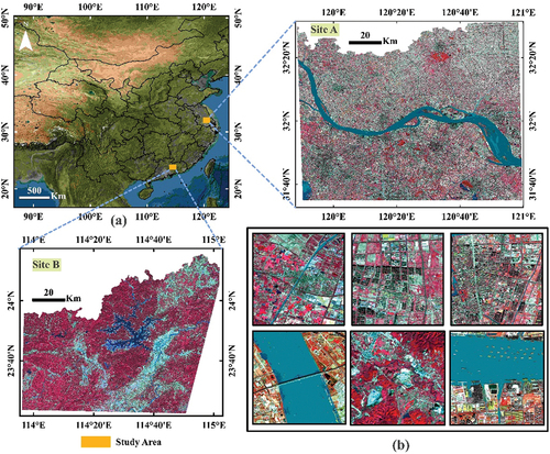
Each of big images was clipped with a 512 × 512 non-overlapping sliding window from the top-left to the right-bottom. A total of 694 images of size 512 × 512 were finally reserved, some of which can be seen in Figure 9(b). The classification scheme used for this study is derived from (Chen et al. 2015), while building shadow is considered in the study area.

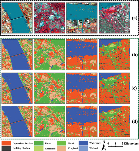
This study employed four pixel-level-based classifiers (Khatami, Mountrakis, and Stehman 2016) including SVM RF and Maximum Likelihood Classification (MLC) (Khatami, Mountrakis, and Stehman 2016; Strahler 1980), k-Nearest Neighbors (KNN) (Franco-Lopez, Ek, and Bauer 2001). These classifiers are highly established, robust, and computationally efficient, exhibiting exceptional performance in classifying medium-resolution multispectral images while utilizing spatial information at the original data scale. To achieve outstanding classification results with experimental images, we employed Object-based Post-classification Refinement (OBPR). This technique enhances the pixel-based classification results with integration of geographic objects delineated from the images using the multiresolution segmentation algorithm embedded in eCognition (Benz et al. 2004, Blaschke 2010). We performed multi-scale segmentation on four spectral bands (i.e. visible R, G, B and Near-infrared) as they provide the highest spatial resolution (10 m). The suitable segmentation parameters were determined through a heuristic process. For each 512 × 512 image, we performed the collection of samples based on the guideline from (Mather 2004). The samples were split into 20% for training, and 80% for validation. Indeed, we collected test data for each 512 × 512 images to calculate classification accuracy metrics. In doing so, we reserved the one having a higher overall classification accuracy. Finally, we found that all classifiers had an average of 90% overall classification accuracy. Figure 10 demonstrates some of them derived from using the Random Forest classifier.

Figure 10. LULCMs derived from MRSI via Random Forest and various decorrelation techniques. The first row: original images in the false-color scheme. The second row: the maps derived from original images. The third row: the LULCM derived from ICA. The fourth row: the maps derived from PCA.

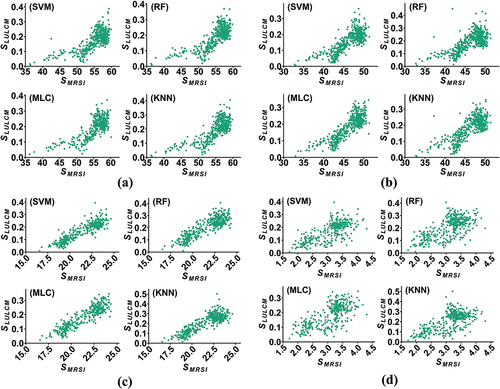
5.2 A nonlinear relationship is found

Figure 11(a) portrays a positive and nonlinear relationship between $S_{MRSI}$ and $S_{LULCM}$ and thus verifies the first hypothesis. This can be easily understood for two given facts, i.e., (i) a heterogenous LULCM (i.e. high $S_{LULCM}$ values) is usually derived from a complicated MRSI (i.e. high $S_{MRSI}$ value) and (ii) given the same classification scheme, the resulting LULCM derived from the same MRSI varies based on the performance of the classifiers used. When MRSI becomes increasingly complicated, $S_{LULCM}$ fluctuates within a range, indicating the upper and lower limits. In addition, we can find that the range of $S_{MRSI}$ is stretched and becomes increasingly smaller as shown in Figures 11(b–d). This shows that the thermodynamic entropy computed by Equation (6)(6) $\begin{array}{c}{S}_{WMRSI}=\sum _{g=1}^G{W}_g\times S_{MRSI}^g\end{array}$(6) is smaller than that calculated by Equation (3)(3) $\begin{array}{c}{S}_{MRSI}=\sum _{\alpha }{S}_R\left(N_1^{\alpha },N_2^{\alpha },\dots ,N_r^{\alpha }\right)\end{array}$(3) . It is worth noting that the relationships shown in Figures 11(c,d) are more linear than these shown in Figures 11(a,b). It indicates that Equation (6)(6) $\begin{array}{c}{S}_{WMRSI}=\sum _{g=1}^G{W}_g\times S_{MRSI}^g\end{array}$(6) could better enhance the mathematical modeling of the information flow.

Figure 11. Scatter plots of $S_{MRSI}$ against $S_{LULCM}$ derived from four classifiers. $S_{MRSI}$ is the thermodynamic entropy of MRSI with or without decorrelation. (a): The original images; (b): ICA is performed on original MRSI; (c): PCA is performed on original MRSI; (d): the weighted thermodynamic entropy in Equation (6)(6) $\begin{array}{c}{S}_{WMRSI}=\sum _{g=1}^G{W}_g\times S_{MRSI}^g\end{array}$(6) is employed to represent $S_{MRSI}$ after performing PCA.

5.3 “Information conservation” is found

Figure 12 demonstrates scatter plots of $F_c$ against W and the fitted models by using the generalized Jarzynski formula. Surprisingly, the mathematic interval of $F_c$ and W values are almost the same. As illustrated in Figure 12(a), the linear models for $F_c$ and W seem excellent as all adjusted R² values are high (i.e. larger than 0.74). Such results significantly support our second hypothesis.

Figure 12. Scatter plots of W against F_c and the fitted thermodynamic-entropy-based Jarzynski models derived from four classifiers. (a) MRSI is not decorrelated; (b) MRSI is decorrelated with ICA; (c) MRSI is decorrelated by PCA, while the information content is not estimated with weights; (d) MRSI is decorrelated by PCA and the information content is the weighted one.

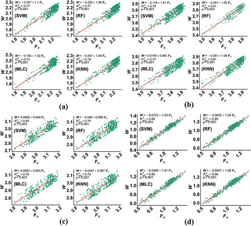
To better facilitate the modeling of energy flow, decorrelation of MRSI is also considered. Concretely, when ICA was employed to decorrelate images, $S_{MRSI}$ in Equation (12)(12) $\begin{array}{rl}{F}_c=& \int \mathrm{\Delta }I\left(pm\right)d\left(pm\right)\\ =& \int \mathrm{\Delta }I\left(S_{imp}^{nu},S_{imp}^{no}\right)d\left(S_{imp}^{nu},S_{imp}^{no}\right)\\ =& S_{MRSI}-S_{LULCM}& (12)\end{array}$(12) is replaced with the one calculated by Equation (5)(5) $\begin{array}{c}{S}_{MMSRI}=\sum _{\mathrm{g}=1}^G\frac{S_{MRSI}^g}{G}\end{array}$(5) . Figure 12(b) shows a similar relationship between $S_{MRSI}$ and $S_{LULCM}$. However, we find that $R_{adj}^2$ values in Figure 12(b) are higher than Figure 12(a), though the range of $F_c$ and W is almost the same.

When PCA is employed to decorrelate the MRSI and the thermodynamic entropy calculated by Equation (6)(6) $\begin{array}{c}{S}_{WMRSI}=\sum _{g=1}^G{W}_g\times S_{MRSI}^g\end{array}$(6) is still used to calculate $F_c$, the performances of the generalized Jarzynski equation in Figure 12(c) are not obviously different from Figure 12(b). This can be attributed to the energy (information) of MRSI represented by $S_{MMRSI}$. Nevertheless, when weighted $S_{MRSI}$ in Equation (7)(7) $\begin{array}{c}\mathrm{\Delta }\mathcal{F}\le W_t\end{array}$(7) is employed to represent the energy (information), the range of $F_c$ becomes narrow. This also indicates that the weighted thermodynamic entropy can well represent the information content of MRSI, thus playing an important role in modeling energy (information) flow. Furthermore, as shown by Figure 12(d), we can find that $R_{adj}^2$ values of the fitted models are the highest (i.e. 0.95), and the generalized Jarzynski equation achieves the best performance. Moreover, in Figure 12(d), we can find that the range of $F_c$ and W derived from three classifiers (i.e. RF, MLC, KNN) are the same. This indicates that “a form of energy (information) conversation” indeed exists in the information flow from MRSI to LULCM.

6. Discussion

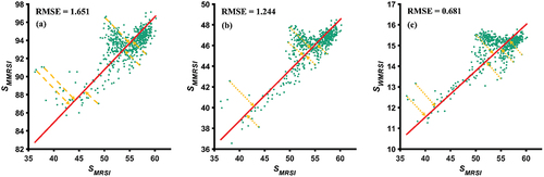
The discussion can be divided into three scenarios. The first scenario is about the information content estimation of a MRSI with thermodynamic entropy. Note that it is inconvenient to perform decorrelation before calculating thermodynamic entropy. Figure 13 addresses this concern, demonstrating a linear relationship between $S_{MRSI}$ and $S_{WMRSI}$ and $S_{MMRSI}$. Hence, we are able to directly use the $S_{MRSI}$ in Equation (3)(3) $\begin{array}{c}{S}_{MRSI}=\sum _{\alpha }{S}_R\left(N_1^{\alpha },N_2^{\alpha },\dots ,N_r^{\alpha }\right)\end{array}$(3) to quantify the information of MRSI without performing decorrelation. 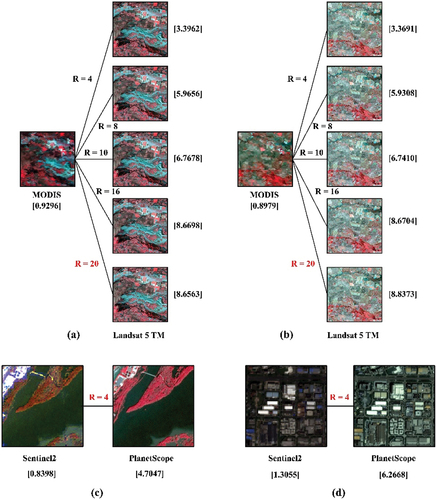This also indicates that the performance of generalized Jarzynski equation shown in Equation (10)(10) $\begin{array}{c}ln{F}_c\le lnW\end{array}$(10) will not be weakened. In addition, by capturing composition and configurational information, thermodynamic entropy can effectively distinguish the information content of MRSI with varying data ranges and different numbers of spectral bands. Consequently, it is anticipated that information flow modeling using thermodynamic entropy can also be extended to diverse sensors (e.g. PlanetScope, Landsat, and MODIS). For example, for the same geographic region, the information content of a MODIS image directly estimated by thermodynamic entropy is far smaller than that of a Landsat 8 image, while their difference may be modeled with the spatial resolution ratio. With information flow modeling, it might be possible to provide a solution for determining the optimal resolution ratio in tasks like spatial-temporal remote sensing image fusion.

Figure 13. The scatter plot of $S_{MRSI}$ against $S_{WMRSI}$, $S_{WMRSI}$ and the fitted models. $S_{WMRSI}$ in (a) and (b) Represent the thermodynamic entropy of MRSI after performing ICA and PCA on images respectively. $S_{WMRSI}$ in (c) Denotes the weighted $S_{MRSI}$ after performing PCA on MRSI.

Figures 14(a,b) illustrate the disparity in information between MODIS and Landsat 5 TM (Emelyanova et al. 2013). As Landsat images become coarser, $S_{MRSI}$ increases. It is noteworthy that the information content of a coarse image should be R (the spatial resolution ratio) times that of a fine one. For example, in Figure 14(a), information content of MODIS should be at least 18.592 (i.e. 0.9296 × 20) bits per pixel. Figures 14(c,d) employ high-resolution images (specifically PlanetScope) to further exemplify the discrepancy in information content with $S_{MRSI}$ as a proxy.

Figure 14. Examples of information content differences represented by $S_{MRSI}$ across three satellite sensors. The $S_{MRSI}$ values are indicated within brackets. The spatial ratio is denoted by R. $S_{MRSI}$ is calculated using bands specifically chosen for land cover classification.

The second scenario is the investigation of information flow across various scales. The utilization of multi-scale information of MRSI plays an essential role in generating high-resolution LULCM (Hua et al. 2021; Ji, Wei, and Lu 2018; Zhao et al. 2023). Fortunately, based on the theoretical and experimental analysis shown in Sections 3 and 4, we are now able to develop an absolute-thermodynamic-entropy-based model to characterize information flow across multiple spatial scales, providing domain knowledge for spatial-temporal remote sensing image fusion (Peng et al. 2021; Shao et al. 2022). In this regard, fluctuation theorems (Crooks 1999) and non-equilibrium thermodynamics can serve as excellent guidelines.

The third scenario is the generality of the thermodynamic-entropy-based Jarzynski equation. Indeed, such generality is highly influenced by the “energy (information) conversion efficiency”, $\eta$. However, there is a tradeoff between the $\eta$ and classifiers and classification schemes (Debats et al. 2016; Dronova et al. 2012), thus influencing the performance of the Jarzynski equation. Therefore, more research is required to address these considerations.

7. Conclusion

Characterizing information flow from MRSI to LULCM is essential for understanding the classification mechanism, providing a foundation of understanding pattern-process relationships and the variation of causality in land cover classification. In this work, we aim to model the information flow with thermodynamic entropy and the law of energy conservation. This study first introduced thermodynamic features of MRSI followed by the description of thermodynamic entropy for MRSI and LULCM. Thereafter, a generalized Jarzynski equation was proposed with thermodynamic entropy to describe the information flow. Six hundred and ninety-four Sentinel-2A MRSI are classified into 10 classes. The experimental results demonstrate three points:

1. the information and thermodynamic features of MRSI and LULCM can be well quantified by thermodynamic entropy.

2. the information flow from MRSI to LULCM is consistent with the law of energy conservation and

3. the information flow from MRSI to LULCM can be described by the generalized Jarzynski equation, which takes the mathematical formula as $W=F_c+W_L$ that contains parameters including the total number of classes, weighted F1-score, and thermodynamic entropies of MRSI and LULCM.

To the best of our knowledge, this study is the first one exploring the use of thermodynamic laws for modeling the transformation of MRSI into LULCM. Compared with previous research concerned with thermodynamic entropy of images, this study involves the definition and modeling of thermodynamic work as well as information flow. Furthermore, it is anticipated that the application of thermodynamic laws and thermodynamic entropy will offer valuable insights into the classification mechanism of MRSI, such as (i) construction of a closed-loop deep-learning-based classification framework, (ii) determination of the optimal number of land cover classes for a given MRSI, and (iii) no-reference quality assessment and reality verification of LULCM at a large spatial-temporal scale.

Disclosure statement

No potential conflict of interest was reported by the author(s).

Data availability statement

Data will be made available upon reasonable request.

Additional information

Funding

This research was supported by the National Natural Science Foundation of China [grant number 41930104] and by the Research Grants Council of Hong Kong [grant number PolyU 152219/18E].

Notes on contributors

Xinghua Cheng

Xinghua Cheng received the MSc degree from The Hong Kong Polytechnic University. He worked as a full-time research assistant at Southwest Jiaotong University from 2022 to 2023. His research interests are information theory, Boltzmann entropy, and remote sensing image processing.

Zhilin Li

Zhilin Li is currently a full professor at Southwest Jiaotong University. He worked as assistant professor, associate professor, full professor, and chair professor at The Hong Kong Polytechnic University from 1996 to 2020, as lecturer at Curtin University from 1994 to 1995, as research fellow/associate at Berlin University of Technology, Southampton University, and Newcastle University from 1990 to 1993. He received his PhD from Glasgow University in 1990. His research interests are geo-information science, cartography and remote sensing image processing.

References

- Benami, E., Z. N. Jin, M. R. Carter, A. Ghosh, R. J. Hijmans, A. Hobbs, B. Kenduiywo, and D. B. Lobell. 2021. “Uniting Remote Sensing, Crop Modelling and Economics for Agricultural Risk Management.” Nature Reviews Earth and Environment 2 (2): 140–159. https://doi.org/10.1038/s43017-020-00122-y.
- Benz, U. C., P. Hofmann, G. Willhauck, I. Lingenfelder, and M. Heynen. 2004. “Multi-Resolution, Object-Oriented Fuzzy Analysis of Remote Sensing Data for GIS-Ready Information.” ISPRS Journal of Photogrammetry and Remote Sensing 58 (3–4): 239–258. https://doi.org/10.1016/j.isprsjprs.2003.10.002.
- Blaschke, T. 2010. “Object Based Image Analysis for Remote Sensing.” ISPRS Journal of Photogrammetry and Remote Sensing 65 (1): 2–16. https://doi.org/10.1016/j.isprsjprs.2009.06.004.
- Boltzmann, L. 1872. “Weitere Studien über das Wärmegleichgewicht unter Gasmolekülen” [Further studies on the thermal equilibrium of gas molecules]. Sitzungsberichte Akademie der Wissenschaften 66: 275–370.
- Carnot, S. 1943. Reflections on the Motive Power of Heat. New York: America Society of Mechanical Engineers.
- Chandler, D. 1987. Introduction to Modern Statistical Mechanics. 1st ed. New York: Oxford University Press, Inc.
- Chen, J., J. Chen, A. P. Liao, X. Cao, L. J. Chen, X. H. Chen, C. H. He, et al. 2015. “Global Land Cover Mapping at 30 M Resolution: A POK-Based Operational Approach.” Isprs Journal of Photogrammetry & Remote Sensing 103: 7–27. https://doi.org/10.1016/j.isprsjprs.2014.09.002.
- Cheng, X. H., and Z. L. Li. 2021a. “Predicting the Lossless Compression Ratio of Remote Sensing Images with Configurational Entropy.” IEEE Journal of Selected Topics in Applied Earth Observations and Remote Sensing 14: 11936–11953. https://doi.org/10.1109/JSTARS.2021.3123650.
- Cheng, X. H., and Z. L. Li. 2021b. “Using Boltzmann Entropy to Measure Scrambling Degree of Grayscale Images.” Paper presented at the Proceedings of the IEEE 5th International Conference on Cryptography, Security and Privacy (CSP), Zhuhai, China, January 8-10. 181–185.
- Congalton, R. 1991. “A Review of Assessing the Accuracy of Classifications of Remotely Sensed Data.” Remote Sensing of Environment 37 (1): 35–46. https://doi.org/10.1016/0034-4257(91)90048-B.
- Crooks, G. E. 1999. “Entropy Production Fluctuation Theorem and the Nonequilibrium Work Relation for Free Energy Differences.” Physical Review E 60 (3): 2721–2726. https://doi.org/10.1103/PhysRevE.60.2721.
- Cushman, S. A. 2016. “Calculating the configurational entropy of a landscape mosaic.” Landscape Ecology 31 (3): 481–489. https://doi.org/10.1007/s10980-015-0305-2.
- Debats, S. R., D. Luo, L. D. Estes, T. J. Fuchs, and K. K. Caylor. 2016. “A Generalized Computer Vision Approach to Mapping Crop Fields in Heterogeneous Agricultural Landscapes.” Remote Sensing of Environment 179: 210–221. https://doi.org/10.1016/j.rse.2016.03.010.
- Dronova, I., P. Gong, N. E. Clinton, L. Wang, W. Fu, S. Qi, and Y. Liu. 2012. “Landscape Analysis of Wetland Plant Functional Types: The Effects of Image Segmentation Scale, Vegetation Classes and Classification Methods.” Remote Sensing of Environment 127: 357–369. https://doi.org/10.1016/j.rse.2012.09.018.
- Emelyanova, I. V., T. R. McVicar, T. G. Van Niel, L. T. Li, and A. I. Van Dijk. 2013. “Assessing the Accuracy of Blending Landsat–MODIS Surface Reflectances in Two Landscapes with Contrasting Spatial and Temporal Dynamics: A Framework for Algorithm Selection.” Remote Sensing of Environment 133: 193–209. https://doi.org/10.1016/j.rse.2013.02.007.
- Fowler, R., and E. A. Guggenheim. 1949. Statistical Thermodynamics. 1st ed. Cambridge: Cambridge University Press.
- Franco-Lopez, H., A. R. Ek, and M. E. Bauer. 2001. “Estimation and Mapping of Forest Stand Density, Volume, and Cover Type Using the K-Nearest Neighbors Method.” Remote Sensing of Environment 77 (3): 251–274. https://doi.org/10.1016/S0034-4257(01)00209-7.
- Fukunaga, K. 1990. Introduction to Statistical Pattern Recognition. Edited by W. Rheinboldt. 2nd San Diego, CA: Academic.
- Gao, P., and Z. Li. 2019. “Computation of the Boltzmann Entropy of a Landscape: A Review and a Generalization.” Landscape Ecology 34 (9): 2183–2196. https://doi.org/10.1007/s10980-019-00814-x.
- Gao, P., H. Zhang, and Z. Li. 2017. “A Hierarchy-Based Solution to Calculate the Configurational Entropy of Landscape Gradients.” Landscape Ecology 32 (6): 1133–1146. https://doi.org/10.1007/s10980-017-0515-x.
- Geman, S., and D. Geman. 1984. “Stochastic Relaxation, Gibbs Distributions, and the Bayesian Restoration of Images.” IEEE Transactions on Pattern Analysis and Machine Intelligence 6 (6): 721–741. https://doi.org/10.1109/TPAMI.1984.4767596.
- Gressman, P. T., and R. M. Strain. 2010. “Global Classical Solutions of the Boltzmann Equation with Long-Range Interactions.” Proceedings of the National Academy of Sciences of the United States of America 107 (13): 5744–5749. https://doi.org/10.1073/pnas.1001185107.
- Guggenheim, E. A. 1967. Thermodynamics. An Advanced Treatment for Chemists and Physicists. 5th ed. New York: Wiley.
- He, H., and E. A. Garcia. 2009. “Learning from Imbalanced Data.” IEEE Transactions on Knowledge and Data Engineering 21 (9): 1263–1284. https://doi.org/10.1109/TKDE.2008.239.
- He, H. S., S. J. Ventura, and D. J. Mladenoff. 2002. “Effects of Spatial Aggregation Approaches on Classified Satellite Imagery.” International Journal of Geographical Information Science 16 (1): 93–109. https://doi.org/10.1080/13658810110075978.
- Heydari, S. S., and G. Mountrakis. 2018. “Effect of Classifier Selection, Reference Sample Size, Reference Class Distribution and Scene Heterogeneity in Per-Pixel Classification Accuracy Using 26 Landsat Sites.” Remote Sens Environment 204: 648–658. https://doi.org/10.1016/j.rse.2017.09.035.
- Hua, Y. S., L. C. Mou, J. Z. Lin, K. Heidler, and X. X. Zhu. 2021. “Aerial Scene Understanding in the Wild: Multi-Scene Recognition via Prototype-Based Memory Networks.” ISPRS Journal of Photogrammetry and Remote Sensing 177: 89–102. https://doi.org/10.1016/j.isprsjprs.2021.04.006.
- Hyvärinen, A., J. Karhunen, and E. Oja. 2001. Independent Component Analysis. 1st ed. Hoboken, NJ, USA: Wiley.
- Jarzynski, C. 1997. “Nonequilibrium Equality for Free Energy Differences.” Physical Review Letters 78 (14): 2690–2693. https://doi.org/10.1103/PhysRevLett.78.2690.
- Ji, S., S. Wei, and M. Lu. 2018. “Fully Convolutional Networks for Multisource Building Extraction from an Open Aerial and Satellite Imagery Data Set.” IEEE Transactions on Geoscience and Remote Sensing 57 (1): 574–586. https://doi.org/10.1109/TGRS.2018.2858817.
- Joule, J. P. 1850. “On the Mechanical Equivalent of Heat.” Philosophical Transactions of the Royal Society 140: 61–82. https://doi.org/10.1098/rstl.1850.0004.
- Jutten, C., and J. Herault. 1991. “Blind Separation of Sources, Part I: An Adaptive Algorithm Based on Neuromimetic Architecture.” Signal Processing 24 (1): 1–10. https://doi.org/10.1016/0165-1684(91)90079-X.
- Khatami, R., G. Mountrakis, and S. V. Stehman. 2016. “A Meta-Analysis of Remote Sensing Research on Supervised Pixel-Based Land-Cover Image Classification Processes: General Guidelines for Practitioners and Future Research.” Remote Sens Environment 177: 89–100. https://doi.org/10.1016/j.rse.2016.02.028.
- Kim, M. H., D. Y. Jeong, and Y. G. Kim. 2021. “Local Climate Zone Classification Using a Multi-Scale, Multi-Level Attention Network.” ISPRS Journal of Photogrammetry and Remote Sensing 181: 345–366. https://doi.org/10.1016/j.isprsjprs.2021.09.015.
- Knopfli, R. 1983. “Coummunication Theory and Generalization.” In Communication and Design in Contemporary Cartography, edited by D. R. Taloyr, 177–218. New York and Chichester: John Wiley & Sons.
- Landauer, R. 1991. “Information is Physical.” Physics Today 44 (5): 23–29. https://doi.org/10.1063/1.881299.
- Li, R., S. Zheng, C. Duan, L. Wang, and C. Zhang. 2022. “Land Cover Classification from Remote Sensing Images Based on Multi-Scale Fully Convolutional Network.” Geo-Spatial Information Science 25 (2): 278–294. https://doi.org/10.1080/10095020.2021.2017237.
- Long, D., and V. P. Singh. 2013. “An Entropy-Based Multispectral Image Classification Algorithm.” IEEE Transactions on Geoscience and Remote Sensing 51 (12): 5225–5238. https://doi.org/10.1109/TGRS.2013.2272560.
- Lu, D., and Q. Weng. 2007. “A Survey of Image Classification Methods and Techniques for Improving Classification Performance.” International Journal of Remote Sensing 28 (5): 823–870. https://doi.org/10.1080/01431160600746456.
- Maldague, M. 2004. “Le deuxie`me principe de la thermodynamique et la gestion de la biosphe`re. Application a` l’environnement et au de´veloppement.” In Traite´ de gestion de l’environnement tropical. Les Classiques des Sciences Sociales, edited by M. Eraift, 10.11–10.21. Saguenay: Les Classiques des Sciences Sociales.
- Ma, L., Y. Liu, X. Zhang, Y. Ye, G. Yin, and B. A. Johnson. 2019. “Deep Learning in Remote Sensing Applications: A Meta-Analysis and Review.” ISPRS Journal of Photogrammetry and Remote Sensing 152: 166–177. https://doi.org/10.1016/j.isprsjprs.2019.04.015.
- Marinoni, A., G. C. Iannelli, and P. Gamba. 2017. “An Information Theory-Based Scheme for Efficient Classification of Remote Sensing Data.” IEEE Transactions on Geoscience and Remote Sensing 55 (10): 5864–5876. https://doi.org/10.1109/TGRS.2017.2716187.
- Mather, P. M.2004. Computer Processing of Remotely-Sensed Images: An Introduction. 3rd ed. Chichester, UK: Wiley.
- Naveh, Z. 1987. “Biocybernetic and Thermodynamic Perspectives of Landscape Functions and Land Use Patterns.” Landscape Ecology 1 (2): 75–83. https://doi.org/10.1007/BF00156229.
- Parrondo, J. M., J. M. Horowitz, and T. Sagawa. 2015. “Thermodynamics of Information.” Nature Physics 11 (2): 131–139. https://doi.org/10.1038/nphys3230.
- Peng, Y. D., W. S. Li, X. B. Luo, J. Du, Y. Gan, and X. B. Gao. 2021. “Integrated Fusion Framework Based on Semicoupled Sparse Tensor Factorization for Spatio-Temporal–spectral Fusion of Remote Sensing Images.” Information Fusion 65: 21–36. https://doi.org/10.1016/j.inffus.2020.08.013.
- Prudente, V. H. R., S. Skakun, L. V. Oldoni, H. A. Xaud, M. R. Xaud, M. Adami, and I. D. Sanches. 2022. “Multisensor approach to land use and land cover mapping in Brazilian Amazon.” Isprs Journal of Photogrammetry & Remote Sensing 189: 95–109. https://doi.org/10.1016/j.isprsjprs.2022.04.025.
- Quan, Y., M. Li, Y. Hao, J. Liu, and B. Wang. 2023. “Tree Species Classification in a Typical Natural Secondary Forest Using UAV-Borne LiDar and Hyperspectral Data.” GIScience & Remote Sensing 60 (1): 2171706. https://doi.org/10.1080/15481603.2023.2171706.
- Shannon, C. E. 1948. “A Mathematical Theory of Communication.” Bell Labs Technical Journal 27 (3): 379–656. https://doi.org/10.1002/j.1538-7305.1948.tb01338.x.
- Shannon, C. E., and W. Weaver. 1972. The Mathematical Theory of Communication. 1st ed. Urbana, Illinois, USA: University of Illinois Press.
- Shao, P., Y. Q. Yi, Z. W. Liu, T. Dong, and D. Ren. 2022. “Novel Multiscale Decision Fusion Approach to Unsupervised Change Detection for High-Resolution Images.” IEEE Geoscience and Remote Sensing Letters 19: 1–5. https://doi.org/10.1109/LGRS.2022.3140307.
- Stephens, G. J., T. Mora, G. Tkačik, and W. Bialek. 2013. “Statistical Thermodynamics of Natural Images.” Physical Review Letters 110 (1): 018701. https://doi.org/10.1103/PhysRevLett.110.018701.
- Stonier, T. 1996. “Information as a Basic Property of the Universe.” Biosystems 38 (2–3): 135–140. https://doi.org/10.1016/0303-2647(96)88368-7.
- Strahler, A. H. 1980. “The Use of Prior Probabilities in Maximum-Likelihood Classification of Remotely Sensed Data.” Remote Sensing Environment 10 (2): 135–163. https://doi.org/10.1016/0034-4257(80)90011-5.
- Szilard, L. 1929. “Über die Entropieverminderung in einem thermodynamischen System bei Eingriffen intelligenter Wesen.” Zeitschrift für Physik 53 (11–12): 840–856. https://doi.org/10.1007/BF01341281.
- Toyabe, S., T. Sagawa, M. Ueda, E. Muneyuki, and M. Sano. 2010. “Experimental Demonstration of Information-To-Energy Conversion and Validation of the Generalized Jarzynski Equality.” Nature Physics 6 (12): 988–992. https://doi.org/10.1038/nphys1821.
- Tuia, D., M. Volpi, L. Copa, M. Kanevski, and J. Munoz-Mari. 2011. “A Survey of Active Learning Algorithms for Supervised Remote Sensing Image Classification.” IEEE Journal of Selected Topics in Signal Processing 5 (3): 606–617. https://doi.org/10.1109/JSTSP.2011.2139193.
- Wang, G., G. Gertner, and A. B. Anderson. 2004. “Up-Scaling Methods Based on Variability-Weighting and Simulation for Inferring Spatial Information Across Scales.” International Journal of Remote Sensing 25 (22): 4961–4979. https://doi.org/10.1080/01431160410001680428.
- Wang, Q., K. S. Song, X. M. Xiao, P. A. Jacinthe, Z. D. Wen, F. R. Zhao, H. Tau, et al. 2022. “Mapping Water Clarity in North American Lakes and Reservoirs Using Landsat Images on the GEE Platform with the RGRB Model.” Isprs Journal of Photogrammetry & Remote Sensing 194: 39–57. https://doi.org/10.1016/j.isprsjprs.2022.09.014.
- Weiss, M., F. Jacob, and G. Duveiller. 2020. “Remote Sensing for Agricultural Applications: A Meta-Review.” Remote Sensing of Environment 236: 111402. https://doi.org/10.1016/j.rse.2019.111402.
- Wheeler, J. A. 1999. “Information, Physics, Quantum: The Search for Links.” In Feynman and Computation: Exploring the Limits of Computers, edited by A. J. G. Hey, 309–336. Reading, MA: Perseus Books.
- White, J. C., T. Hermosilla, M. A. Wulder, and N. C. Coops. 2022. “Mapping, Validating, and Interpreting Spatio-Temporal Trends in Post-Disturbance Forest Recovery.” Remote Sensing of Environment 271: 112904. https://doi.org/10.1016/j.rse.2022.112904.
- Zhao, Y. L., C. Y. Diao, C. K. Augspurger, and Z. J. Yang. 2023. “Monitoring Spring Leaf Phenology of Individual Trees in a Temperate Forest Fragment with Multi-Scale Satellite Time Series.” Remote Sensing of Environment 297: 113790. https://doi.org/10.1016/j.rse.2023.113790.
- Zhong, Y., A. Ma, and L. Zhang. 2014. “An Adaptive Memetic Fuzzy Clustering Algorithm with Spatial Information for Remote Sensing Imagery.” IEEE Journal of Selected Topics in Applied Earth Observations and Remote Sensing 7 (4): 1235–1248. https://doi.org/10.1109/JSTARS.2014.2303634.
- Zhong, Y. F., B. W. Yan, J. J. Yi, R. Y. Yang, M. Z. Xu, Y. Su, Z. D. Zheng, and L. P. Zhang. 2023. “Global Urban High-Resolution Land-Use Mapping: From Benchmarks to Multi-Megacity Applications.” Remote Sensing of Environment 298: 113758. https://doi.org/10.1016/j.rse.2023.113758.
- Zhou, W., C. Persello, M. M. Li, and A. Stein. 2023. “Building Use and Mixed-Use Classification with a Transformer-Based Network Fusing Satellite Images and Geospatial Textual Information.” Remote Sensing of Environment 297: 113767. https://doi.org/10.1016/j.rse.2023.113767.