Dual-environment feature fusion-based method for estimating building-scale population distributions

ABSTRACT

Information on the population distribution at the building scale can help governments make supplemental decisions to address complex urban management issues. However, the discontinuity and strong spatial heterogeneity of research units at the building scale make it challenging to fuse multi-source geographic data, which causes significant errors in population estimation. To address this problem, this study proposes a method for population estimation at the building scale based on Dual-Environment Feature Fusion (DEFF). The dual environments of buildings were constructed by splitting the physical boundaries and extracting features suitable for the dual-environment scale from multi-source geographic data to describe the complex environmental features of buildings. Meanwhile, Data Quality Weighting based Technique for Order of Preference by Similarity to Ideal Solution (DQW-TOPSIS) method was proposed to assign appropriate weights to the features of the external environment for better feature fusion. Finally, a regression model was established using dual-environment features for building-scale population estimation. The experimental areas chosen for this study were Jianghan and Wuchang Districts, both located in Wuhan City, China. The estimated results of the DEFF were compared with those of the ablation experiments, as well as three publicly accessible population datasets, specifically LandScan, WorldPop, and GHS-POP, at the community scale. The evaluation results showed that DEFF had an $R^2$ of approximately 0.8, Mean Absolute Error (MAE) of approximately 1200, Root Mean Square Error (RMSE) of approximately 1700, and both Mean Absolute Percentage Error (MAPE) and Symmetric Mean Absolute Percentage Error (SMAPE) of approximately 26%, indicating an improved performance and verifying the validity of the proposed method for fine-scale population estimation.

KEYWORDS:

• Building scale
• multi-source data fusion
• estimation of population distribution
• dual environment
• Data Quality Weighting based Technique for Order of Preference by Similarity to Ideal Solution (DQW-TOPSIS)

1. Introduction

Precise population data are a fundamental component of effective urban administration and strategic planning. Population distribution data with precise spatial and temporal resolutions are being increasingly employed in several domains of urban development management, including disaster assessment, traffic planning, and resource allocation (Meng et al. 2021; Zhang et al. 2022). The most reliable and comprehensive information on population distribution often originates from national censuses. However, censuses are updated at long intervals, and the statistical scale of administrative districts is relatively coarse, which can hardly reflect the heterogeneity of population distribution within statistical units (Gui et al. 2022), and thus cannot fulfill the requirements of fine-grained urban management. Therefore, the population density modeling method (Lv et al. 2002), spatial interpolation method (Liu, Kyriakidis, and Goodchild 2008; Lv et al. 2002; Mennis 2009), and statistical modeling methods (Gui et al. 2022; Loh and Shin 1997; Meng et al. 2021; Shang et al. 2021; Wang et al., 2022) have been successively established from the perspectives of geography, economics, and statistics, thus refining the spatial scale of population distribution.

The regular shape and consistent distribution of grid cells facilitate the feature fusion and scale transformation of multisource geospatial data, making it a commonly used unit for population modeling (Li and Peng 2007; Meng et al. 2021; Shang et al. 2021; Wang et al., 2022). However, real-world urban structures exhibit complex morphological features. Geographical entities, such as building patches, are irregular in shape and discretely distributed. Consequently, a grid cell often includes only a part of a geographical entity or can consist of multiple geographic entities, leading to ambiguity in its geographical properties. The utilization of building patches as basic units offers more precise geographic attributes and meets the needs of fine urban management better than grid cells. Therefore, the building scale has become a new trend in the study of scales for population estimation (Lin and Zhang 2017; Balakrishnan 2020; Xia et al. 2021).

There have been numerous methods for estimating building-scale population distributions, such as directly extracted features at the building scale, including statistical modeling (Liu et al. 2021; Meng et al. 2021), spatial interpolation (Shang et al. 2021), meta cellular automata (Min et al. 2019), and gravity models (Yao et al. 2017). However, some of these methods ignore the fact that building scales are discontinuous, which not only results in the loss of valuable data but also complicates the feature fusion step. An alternative strategy involves using dasymetric methods to assign modeling outcomes from the regular grid scale to the building scale, despite the resulting scale mismatch problem. Mei et al. (2022) proposed a Cross-Scale Feature Construction method to reduce the population heterogeneity owing to pixel-level attribute discretization, which provides a new method for constructing population-related features across scales. Generally, extracting features from multi-source geospatial data and fusing them effectively are key issues in estimating building-scale population distribution.

When extracting building-scale features, two types of features can be applied for population estimation: a building’s intrinsic characteristics and its surroundings. The intrinsic characteristics of a building related to its population distribution primarily include its floor, area, and function type (Wang et al. 2021). Obtaining the functional types of buildings directly can be challenging; therefore, land-use data or Points Of Interest (POI) data are commonly used to identify the functional type of a building (Chen, Zhou, and Wu 2020; Cao et al. 2020; Wang et al. 2021). In addition, the external environment surrounding the building influences the occupancy rate of the population to some extent, and it can usually be represented by other geospatial data sources, such as POI data (Zhao et al. 2019), mobile signaling data (Kubíček et al. 2019), and nighttime light data (Han et al. 2019; He, Pan, and Dong 2020; Zhang et al. 2021). Different types of data features must be expressed on optimal scales.

To alleviate the feature fusion scale problem that affects building-scale population estimation, we introduced the concept of dual environments for buildings. The dual environment includes both the internal and external environments of the building. The boundary of the internal environment corresponds to the building shape, whereas the boundary of the external environment is defined by the Traffic Analysis Zone (TAZ) to which the building belongs. The features representing the dual environments of the building were extracted on dual scales. Thus, we can consider the collective influence of both buildings and their surroundings on the population distribution. We chose Jianghan and Wuchang Districts in Wuhan City, China, as our research areas. We then developed a building-scale population distribution estimation method based on Dual-Environment Feature Fusion (DEFF). Specifically, to provide a suitable spatial scale for multi-source geographical data feature extraction, the internal and external physical environment boundaries of the buildings were constructed. Considering the influence of a building’s function on its population capacity, we identified the building’s function based on the dual environment and degree of public awareness (Chi et al. 2016) and calculated the population capacity of the inner environment using the building’s floor and area features. In addition, considering that the external environment of a building reflects the population’s intention to live to some extent, we calculated the population capacity of the building’s external environment using the proposed Data Quality Weighting based Technique for Order of Preference by Similarity to Ideal Solution (DQW-TOPSIS) method. Finally, a linear regression model was constructed based on dual-environment features to obtain the building-scale population distribution.

This study offers the following innovations and contributions.

1. Concept of dual environments: We introduced the concept of dual environments for buildings. The internal environment captures the intrinsic features of a building, whereas the external environment addresses information loss when features are directly extracted from multi-source data at the building scale. Dual environments also provide an appropriate feature-representation scale for multisource data fusion.

2. Building function type identification: We proposed a hierarchical process for identifying the building function types. Utilizing building, TAZ, and land use data at different levels, we identified building function types based on the public awareness of POI types. This approach can enhance the effectiveness of the features for building-scale population modeling.

3. Enhanced TOPSIS method: We enhanced the TOPSIS method by incorporating the DQW. This enhancement allowed us to set reasonable fusion weights for external environmental features based on data quality, thereby improving the fusion of multi-source data features.”

2. Methodology

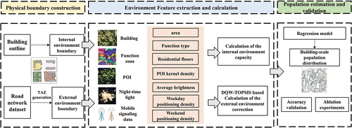
Buildings exist in a variety of natural and artificial environments. The features of these external environments interact with those of the buildings themselves, thereby influencing population distribution at the building scale. Accordingly, we propose the DEFF method. The overall building-scale population distribution estimation method based on the DEFF is shown in Figure 1 and comprises four main steps: constructing the dual environmental physical boundaries of buildings, calculating the population capacity of the internal environment, calculating population corrections based on the external environment, and estimating the population distribution.

Figure 1. Workflow of the proposed DEEF method.

1) Construction of dual-environment physical boundaries for buildings

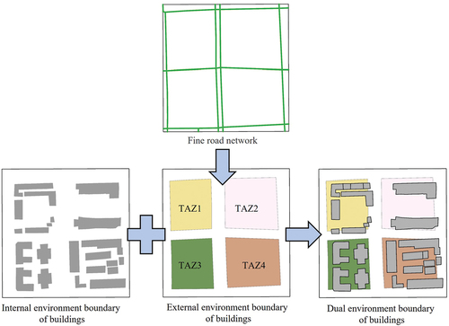
Several factors influence the building population, extending beyond the building itself to the surrounding environment. To comprehensively evaluate the combined influence of a building and its surroundings on the population distribution, we established internal and external environmental boundaries for the building. The internal boundary corresponded to the contour of the building patch, whereas the external boundary was aligned with the Traffic Analysis Zone (TAZ). The TAZ boundary was constructed using fine-scale road network data, which provides a suitable spatial scale for feature calculation when integrating multi-source geospatial data at the building scale.

2) Calculation of the population capacity of the internal environment

The shape, function type, volume, and other features of a building are closely related to its population capacity (Metzger et al. 2022). To quantify this influence of a building’s internal environment, we introduced a metric known as “population capacity.” It is computed from three features of the building’s internal environment: the number of floors, total area, and building function type. In addition, we devised a progressive process to identify residential buildings.”

3) Calculation of population corrections based on the external environment

The external environment of a building affects its population. Assuming two residential buildings with the same floors and areas-one in the center of the city and one in the suburbs – it is conceivable that the population occupancy rate of the former building will be higher than that of the latter because the external environments of the two buildings are different. Therefore, we extracted the features of POI, mobile phone signaling, and nighttime lighting data at the TAZ scale to describe the external environment of each building. We then applied the DQW-TOPSIS method to calculate the population correction for the external environment.

4) Estimation of population distribution

Using the population capacity of the internal environment of a building as the main factor and the population correction quantity of the external environment as a supplementary factor, a linear regression method was established to construct a building-scale population distribution model.

2.1. Construction of dual environment physical boundaries of buildings

In the modeling process, we defined a building’s dual environment with internal and external boundaries. The internal environmental boundary of a building is defined as a contour boundary. Buildings serve as the basic independent units that accommodate the population, offering a finer and more accurate representation of population distribution than grid cells. Factors, such as the functional type, number of floors, area, shape, and other features, significantly influence a building’s population capacity.

However, it is important to acknowledge that buildings do not exist in isolation but rather within diverse natural and man-made contexts. These external environments usually exert a substantial impact on the occupancy rate of residential buildings (Han et al. 2019), thereby influencing the population distribution. Therefore, it is necessary to consider the influence of the external environment on the actual occupancy of a building when estimating the building-scale population. In addition, in the feature extraction process, owing to the fine scale and discontinuity of building units, proper representation of some geospatial data features related to population distribution remains challenging at the building scale. For example, nighttime light data often exhibit a spatial spillover effect, as the actual light emitted by a building usually extends beyond its physical boundaries and affects the surrounding area; thus, the features are better suited for calculations at continuous or larger scales. The same issue arises with other data types, such as the radius of a restaurant’s POI serving more than the building itself. To alleviate the spatial offset of the point data, we employed both coordinate correction techniques and kernel density processing on the point data. In summary, buildings are discrete microscopic units, and calculating features directly at this scale can result in information loss. Considering the limitation of multiscale data fusion and the necessity for external environmental features, our approach introduces external environmental boundaries for buildings for effective geospatial data feature fusion. Several studies have verified that, in comparison to administrative districts, such as streets and communities, urban land parcels split based on road networks offer a more effective representation of the actual construction forms of cities (Yang, Fang, and Yin 2018), and they are commonly used units for urban function division (Chen et al. 2020). Therefore, we defined the external environmental boundary of a building as the boundary of the TAZ in which it is located, and the buildings within the same TAZ share the same external environment. Based on previous studies (Chi et al. 2016; Chen et al. 2022), ArcMap 10.8 desktop software was used to process detailed road network data and obtain the TAZs of our study area. Figure 2 illustrates the process of generating a dual-building environment.

Figure 2. Illustration of building environment generation process.

2.2. Calculation of the internal environment population capacity

Typically, the features of a building are related to its population distribution, including area, number of floors, function type (Dong, Yang, and Cai 2016), and shared common area (Wang et al. 2021). The area and number of floors in a building enable the calculation of its volume, which directly reflects its maximum population capacity. The actual population capacities of buildings vary widely among the different function types (Li, Wang, and Dong 2013). However, building function features, such as area and floor features, cannot be easily identified based on remote sensing images, and additional auxiliary data are usually required. In most studies, land-use and POI data have been used to identify building functions. For example, Wang et al. (2021) reclassified POIs into commercial, residential, and public types, and identified residential buildings using the term frequency-inverse document frequency algorithm. Cao et al. (2020) assigned inverse distance weights to POIs inside buildings and their buffers and calculated the weighted frequency density ratios for different types of POIs to identify building types. However, these studies treated the integrated environmental semantics of POIs on a single buffer zone scale as the functional semantics of buildings, thereby deviating from the actual situation and reducing the accuracy of building classification. To address this issue, in addition to the internal and external physical environment boundaries constructed above, public awareness (Zhao, Li, and Li 2011) can be used to obtain the integrated environmental semantics from the POIs within the dual environments, thus calculating the number of habitable floors in residential and mixed-type buildings. The detailed residential building identification process is illustrated in Figure 3.

Figure 3. Flow chart illustrating the residential building identification process.

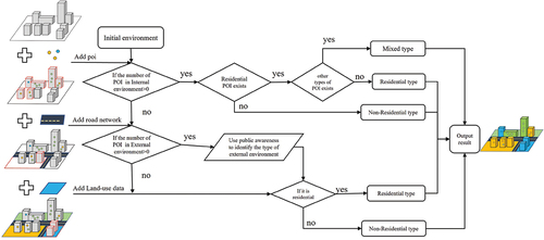
First, we identified the internal environmental semantics of the building itself based on the following criteria: if there were only nonresidential POIs, the building was classified as a nonresidential building; if there were residential and other types of POIs, the building was classified as a mixed-type building. In this case, the actual number of habitable floors $f_{resi}$ was equal to the total number of floors $f_{all}$ reduced by one, i.e. $f_{resi}=f_{all}-1$, as the first floor of a mixed-type building usually contains convenience stores or restaurants; if only residential POIs existed, the building was a residential building.

When there was no POI in a building to aid in identifying its functional semantics, the environmental boundary of the building was extended to the external environmental boundary, because the surrounding environments often exhibited similarities in certain features. Consequently, a building’s environmental function relies on public awareness, which is a commonly employed method for identifying urban functional areas. In accordance with China’s urban land classification standards, urban functional areas are classified into six distinct categories: residential, public administration and service, commercial service, industrial, road transportation facility, greening, and park areas (Hu et al. 2022). We utilized the public awareness of each type of POIs and the mapping tables between POIs and urban functional area types and chose the urban functional area type with the highest percentages as the functional categories of the building environments. In Equation (1)(1) $F{T}_q=\sum _{p\in P_q}{N}_p\times A{w}_p$(1) , $F{T}_q$ represents the statistical frequency of urban functional area type $q$, $P_q$ is the set of POI types belonging to $q$, $N_p$ is the number of POI type $p$, and $A{W}_p$ is the public awareness value of $p$. In Equation (2)(2) $FT=max\left\{F{T}_1,F{T}_2,\cdots ,F{T}_6\right\}$(2) , $FT$ denotes the maximum statistical frequency of the urban functional area type. The urban functional area type tied to $FT$ is a building’s environmental function type. If the corresponding type of $FT$ is residential, the building is classified as residential; otherwise, it is classified as nonresidential.

In cases where there was no POI inside both the internal and external environments of a building, land use data were utilized as a supplementary means of assessment. The classification of a building as residential or nonresidential was determined by its land use category.

Through comprehensive consideration of the three situations outlined above, we achieved an effective classification of buildings. The habitability coefficient ($C_i$) was calculated for each building based on its function types, allowing the quantification of its capacity to house populations. The mapping relationships between the functional types of buildings and their habitability coefficients are listed in Table 1.

(1) $F{T}_q=\sum _{p\in P_q}{N}_p\times A{w}_p$(1)

(2) $FT=max\left\{F{T}_1,F{T}_2,\cdots ,F{T}_6\right\}$(2)

Table 1. Building type and habitability coefficient mapping relationships.

Building type	Habitability coefficient $C_i$
Residential building	1
Mixed-use building	$\frac{f_{all}-1}{f_{all}}$
Non-residential building	0

The next step was to establish the population capacity index of the building’s internal environment using Equation (3)(3) $E\mathrm{\_}i{n}_i=C_i\times f_{all}\times a$(3) to combine the building’s three features: number of floors, area, and habitability coefficient $C_i$:

(3) $E\mathrm{\_}i{n}_i=C_i\times f_{all}\times a$(3)

where $E\mathrm{\_}i{n}_i$ represents the internal environment population capacity of the $i\text{-}\mathrm{t}\mathrm{h}$ building, $C_i$ represents the habitability coefficient, $f_{all}$ represents the total number of floors in the $i\text{-}\mathrm{t}\mathrm{h}$ building, $f_{resi}$ represents the number of residential floors in the $i\text{-}\mathrm{t}\mathrm{h}$ building, and $a$ represents the cover area of the building.

Equation (3)(3) $E\mathrm{\_}i{n}_i=C_i\times f_{all}\times a$(3) indicates that the population capacity of a building’s internal environment was determined by distinct rules based on the building type.

For residential buildings, the habitability coefficient was set to 1, and the population capacity was calculated as the product of the number of floors and the building area.

In the case of mixed-use buildings, the habitability coefficient was defined as the ratio of residential floors to the total number of floors, and the population capacity was computed as the product of the number of residential floors and the building area.

For nonresidential buildings, the habitability coefficient was set to 0, resulting in a population capacity of 0.

2.3. Calculating population corrections for external environments

In addition to the intrinsic characteristics of buildings, the external environment of a building influences its population (Li et al. 2021). The external environment of a building can usually be reflected by geospatial big data, such as POI data, mobile phone signaling data, and nighttime light data. Several studies have shown that areas with denser POIs tend to have a higher frequency of population activity, and the active mobile phone data collected can describe the real-time population distribution (Mileu, Queirós, and Morgado 2022). The intensity of nighttime lights can also serve as an indicator of the housing vacancy rate, thereby improving the accuracy of population distribution estimation and the actual population distribution to some extent (Han et al. 2019; He, Pan, and Dong 2020).

Given these considerations, we utilized four features to characterize the external environments of buildings: total nighttime light brightness value, total POI kernel density, and total nighttime mobile signaling data on both weekdays and weekends. The choice of scale for constructing these features has been extensively explored in existing research. Drawing upon insights from prior studies and considering the characteristics of our collected data, we processed all the features to the 100-m scale and aggregated them to the TAZ scale for our modeling. Based on the basic TOPSIS method (Lai, Liu, and Hwang 1994), we proposed DQW-TOPSIS, a new method for evaluating a building’s external environment. The external environment of a building can be evaluated by assessing the proximity of its feature values of the external environment to the optimal feature values. Unlike the original TOPSIS method, which treats all features equally, our proposed DQW-TOPSIS method assigns weights to external environmental features based on data quality. This weighting scheme enhanced the fusion of data from various sources and contributed to a more accurate assessment. The fundamental steps of this method are illustrated in Figure 4.

Figure 4. Flow chart illustrating the residential building identification process.

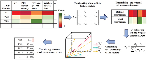
(1) Construction of the standardized feature matrix

First, each external environment was expressed using $m$ features. Then, a normalized weight matrix with $n$ rows and $m$ columns was constructed from the feature vectors of $n$ external environment. The $m$ features in this study were total nighttime light brightness, total POI kernel density, total nighttime mobile signaling on weekdays, and total nighttime mobile signaling on weekends, that is, $m=4$.

(2) Determination of the optimal and worst environment vectors

The optimal environment vector ${\mathit{Z}}^{\mathbf{+}}$ was defined as a vector in which each environment feature was assigned its highest value, while the worst environment vector was defined as a vector ${\mathit{Z}}^{\mathbf{-}}$ in which each environment feature was assigned its minimum value.

(3) Construction of weights of features based on DQW

The effectiveness of data–feature fusion is often constrained by data quality. Therefore, it is necessary to adjust the weights in accordance with the quality of the data (Wang et al., 2022). However, the conventional TOPSIS method assumes that all the feature weights are equally important. Therefore, we introduced a step called DQW, which assigns weights to external environmental features based on data quality. The data quality was measured based on the informativeness and reliability of the data. The informativeness of a data feature is described by its internal variance in external environments, as denoted by Equations (5)(5) ${\sigma }_{ij}=\sum _{i=1}^n\frac{{\sum }_{p=1}^q{\left(v_{ijp}-\bar{v}\right)}^2}{q}$(5) and (6(6) $r_j=\frac{n\left(\mathrm{\Sigma }{x}_i{y}_i\right)-\left(\mathrm{\Sigma }{x}_i\right)\left(\mathrm{\Sigma }{y}_i\right)}{\begin{array}{c}\sqrt{\left[n\mathrm{\Sigma }{x}_i^2-{\left(\mathrm{\Sigma }{x}_i\right)}^2\right]\left[n\mathrm{\Sigma }{y}_i^2-{\left(\mathrm{\Sigma }{y}_i\right)}^2\right]}\end{array}}$(6) ):

(4) ${\sigma }_j=\sum _{i=1}^n{\sigma }_{ij}$(4)

(5) ${\sigma }_{ij}=\sum _{i=1}^n\frac{{\sum }_{p=1}^q{\left(v_{ijp}-\bar{v}\right)}^2}{q}$(5)

where ${\sigma }_j$ represents the informativeness of the $j\text{-}\mathrm{t}\mathrm{h}$ external environment feature, ${\sigma }_{ij}$ represents the variance of the $j\text{-}\mathrm{t}\mathrm{h}$ feature in the $i\text{-}\mathrm{t}\mathrm{h}$ external environment, $v_{ijp}$ represents the value of the $j\text{-}\mathrm{t}\mathrm{h}$ feature in the $p\text{-}\mathrm{t}\mathrm{h}$ pixel of the $i\text{-}\mathrm{t}\mathrm{h}$ building environment, and $\bar{v}$ is the mean value of$\hspace{0.17em}$ the $j\text{-}\mathrm{t}\mathrm{h}$ feature in the $i\text{-}\mathrm{t}\mathrm{h}$ building environment.

The reliability of a data feature is described by the Pearson’s correlation coefficient (r) between itself and the population, as shown in Equation (6)(6) $r_j=\frac{n\left(\mathrm{\Sigma }{x}_i{y}_i\right)-\left(\mathrm{\Sigma }{x}_i\right)\left(\mathrm{\Sigma }{y}_i\right)}{\begin{array}{c}\sqrt{\left[n\mathrm{\Sigma }{x}_i^2-{\left(\mathrm{\Sigma }{x}_i\right)}^2\right]\left[n\mathrm{\Sigma }{y}_i^2-{\left(\mathrm{\Sigma }{y}_i\right)}^2\right]}\end{array}}$(6) .

(6) $r_j=\frac{n\left(\mathrm{\Sigma }{x}_i{y}_i\right)-\left(\mathrm{\Sigma }{x}_i\right)\left(\mathrm{\Sigma }{y}_i\right)}{\begin{array}{c}\sqrt{\left[n\mathrm{\Sigma }{x}_i^2-{\left(\mathrm{\Sigma }{x}_i\right)}^2\right]\left[n\mathrm{\Sigma }{y}_i^2-{\left(\mathrm{\Sigma }{y}_i\right)}^2\right]}\end{array}}$(6)

where $r_j$ represents the reliability of the $j\text{-}\mathrm{t}\mathrm{h}$ external environmental features and $x_i$ represents the sum of the $j\text{-}\mathrm{t}\mathrm{h}$ feature values in the $i\text{-}\mathrm{t}\mathrm{h}$ community, where $y_i$ is the real population of this community.

By combining ${\sigma }_j$ and $r_j$, the fusion weight of the $j\text{-}\mathrm{t}\mathrm{h}$ feature can be calculated using Equation (7)(7) $w_j=\frac{{\sigma }_j\times r_j}{{\sum }_{j=1}^n{\sigma }_j\times r_j}$(7) .

(7) $w_j=\frac{{\sigma }_j\times r_j}{{\sum }_{j=1}^n{\sigma }_j\times r_j}$(7)

(4) Calculation of the distances between environment vectors and the ideal or worst environmental vectors

Euclidean distance was employed to assess the similarity between the feature vectors of the external environment and the vectors representing the optimal or worst environment. The distance between the $i\text{-}\mathrm{t}\mathrm{h}$ $\left(i=1,2,\cdots ,n\right)$ external environment vector and optimal environment vector is denoted by $D_i^{+}$ in Equation (8)(8) $D_i^{+}=\sqrt{\sum _{j=1}^m{w}_j{\left(Z_j^{+}-z_{ij}\right)}^2}$(8) . Similarly, the distance between the $i\text{-}\mathrm{t}\mathrm{h}$ $\left(i=1,2,\cdots ,n\right)$ external environment vector and the worst environment vector is denoted as $D_i^{-}$ in Equation (9)(9) $D_i^{-}=\sqrt{\sum _{j=1}^m{w}_j{\left(Z_j^{-}-z_{ij}\right)}^2}$(9) .

(8) $D_i^{+}=\sqrt{\sum _{j=1}^m{w}_j{\left(Z_j^{+}-z_{ij}\right)}^2}$(8)

(9) $D_i^{-}=\sqrt{\sum _{j=1}^m{w}_j{\left(Z_j^{-}-z_{ij}\right)}^2}$(9)

(5) Calculation of the external environment population correction

The calculated $D_i^{+}$ and $D_i^{-}$ in previous step were used to obtain the external environment population correction for the buildings within the $i\text{-}\mathrm{t}\mathrm{h}$ external environment, as shown in Equation (10)(10) $E\mathrm{\_}ou{t}_i=\frac{D_i^{-}}{D_i^{+}+D_i^{-}}$(10) .

(10) $E\mathrm{\_}ou{t}_i=\frac{D_i^{-}}{D_i^{+}+D_i^{-}}$(10)

From Equation (10)(10) $E\mathrm{\_}ou{t}_i=\frac{D_i^{-}}{D_i^{+}+D_i^{-}}$(10) , it can be readily inferred that $0\le E\mathrm{\_}ou{t}_i\le 1$, and the smaller $D_i^{+}$ is, the larger $E\mathrm{\_}ou{t}_i$ is.

2.4. Estimating the population distribution

To comprehensively consider the effects of the building’s internal environment discussed in Section 2.2 and external environment discussed in Section 2.3 on the population distribution, multiple linear regression method was employed. The least-squares method was used to solve the regression coefficient of the model based on the premise that the sum of the squares of the residuals between the estimated and real populations was minimized. The DEFF regression model is given by Equation (11)(11) $po{p}_k=a\times {\sum }_{i=0}^{n}E\mathrm{\_}i{n}_i+b\times {\sum }_{i=0}^{n}E\mathrm{\_}ou{t}_i$(11) :

(11) $po{p}_k=a\times {\sum }_{i=0}^{n}E\mathrm{\_}i{n}_i+b\times {\sum }_{i=0}^{n}E\mathrm{\_}ou{t}_i$(11)

where $po{p}_k$ is the estimated population of the $k\text{-}\mathrm{t}\mathrm{h}$ community; $E\mathrm{\_}i{n}_i$ is the internal environment population capacity of the $i\text{-}\mathrm{t}\mathrm{h}$ $\left(i=1,2,\cdots ,n\right)$ building in the $k\text{-}\mathrm{t}\mathrm{h}$ community, which is calculated using Equations (1)(1) $F{T}_q=\sum _{p\in P_q}{N}_p\times A{w}_p$(1) –(3(3) $E\mathrm{\_}i{n}_i=C_i\times f_{all}\times a$(3) ); $\hspace{0.17em}E\mathrm{\_}ou{t}_i$ is the population correction for the external environment of the $i\text{-}\mathrm{t}\mathrm{h}$ building, which is derived using Equations (4)(4) ${\sigma }_j=\sum _{i=1}^n{\sigma }_{ij}$(4) –(10(10) $E\mathrm{\_}ou{t}_i=\frac{D_i^{-}}{D_i^{+}+D_i^{-}}$(10) ); and $a$ and $b$ are the regression coefficients.

To verify the effects of the building’s internal and external environmental features, the building function identification method, and the DQW-TOPSIS module of our population estimation model, DEFF, we modified the model parameters in DEFF and performed ablation experiments.

DEFF1: considers only the internal population capacity of a building. Therefore, b in (11) is equal to zero.

DEFF2: considers only the external environmental features of the buildings. Therefore, a in (11) is equal to zero.

DEFF3: considers both the internal and external environmental features of buildings but ignores the function types of buildings, that is, it allows $C_i$ in Equation (3)(3) $E\mathrm{\_}i{n}_i=C_i\times f_{all}\times a$(3) to always be 1.

DEFF4: considers both the internal and external environment features of buildings but uses the original TOPSIS method to calculate the external environment population correction. Therefore, each feature of the building’s external environment was weighed equally.

In addition, to verify that our model provides appropriate scales for feature extraction and the effectiveness of the DQW-TOPSIS method for feature fusion, we constructed two baselines based on the linear regression method for comparison.

LR(building): Existing studies on building-scale population distributions usually extract features directly at the building scale (Shang et al. 2021). To demonstrate the effectiveness of extracting population-related features at the dual-environment scale, we extracted all features at the building scale and did not use DQW-TOPSIS for feature fusion; instead, we directly used these features as independent variables in a multiple linear regression model, which is denoted as LR(building).

LR(TAZ): To verify the effectiveness of the DQW-TOPSIS method when fusing external environmental features, we extracted all external environmental features at the TAZ scale like DEFF, but did not use DQW-TOPSIS for feature fusion; instead, we directly used these features as independent variables in the multiple linear regression model, which is denoted as LR(TAZ).

3. Study area and data sources

3.1. Study area

As a polycentric city, each block in Wuhan in Hubei province has its own development features and directions according to local conditions. Jianghan and Wuchang Districts are located in the center of the left and right banks of the main axis of the Yangtze River, respectively, and are part of the center of Wuhan City. The geographical location of the study area is shown in Figure 5.

Figure 5. Overview of the study area Jianghan District and Wuchang District in Wuhan. (a) Location of Wuhan in Hubei Province. (b) Location of Jianghan District and Wuchang District in Wuhan. (c) Building units represent the study area.

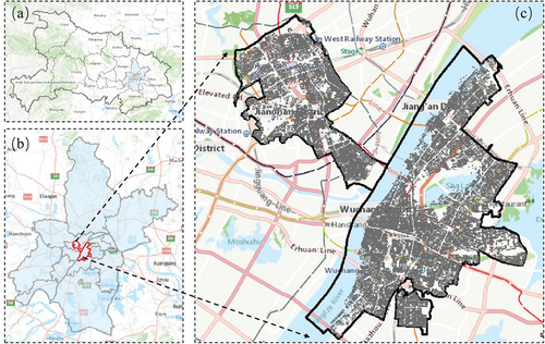
Jianghan District covers an area of 28.29 km², with a resident population of 683,492 in 2015. In 2021, the annual GDP of the district reached 143.8 billion yuan, and the economic density, population density, and output per unit area ranked first among all of the urban areas in Wuhan. Jianghan District has a well-developed commercial and financial industry, and a cultural tourism industry based on its characteristic history and culture of Jianghan District has been formed. Wuchang District has a long history and culture, a beautiful natural environment, rich tourism resources, solid scientific and educational facilities, and comprehensive economic strength. At present, the urbanization rate in Wuchang District is 100%, the jurisdictional area is 107.76 km², and the resident population was approximately 1,199,200 in 2015; thus, the population density is high.

Experiments were conducted on 107 communities in Jianghan District and 191 communities in Wuchang District, China. Jianghan and Wuchang Districts have comprehensive urban functions, including old urban areas, commercial urban areas, green landscapes, medical service areas, and cultural and educational areas, which are representative of complex urban population models. In addition, to further ensure the generality of the model, the natural breaks method was used to divide the communities into high, medium, and low types by population size when dividing the training and test sets; the division ratio of the training and test sets was 3:1.

3.2. Data sources

The multi-source geospatial data used in our experiments are shown in Table 2 and can be divided into real data, auxiliary modeling data, and validation data. Census data used as real data are the most authoritative sources of population data in China. The auxiliary modeling data included POI, building, road network, mobile signaling, land use, and nighttime light data. WorldPop (Lloyd et al. 2020), GHS-POP (Freire et al. 2016), and LandScan data (Bright, Rose, and Urban 2016) were used for validation.

Table 2. Type, source, and year of the experimental data.

Data type	Data Name	Data source	Year
Real data	Census population data	Wuhan Statistical Yearbook, Wuhan Community Demographic Census	2015
Auxiliary data	Point-of-interest data	Gaode Map (https://www.amap.com/)	2015
	Building data	Wuhan Land Use and Urban Spatial Planning Research Center	2016
	Road network	Gaode Map (https://www.amap.com/)	2018
	Cellular signaling data	http://wayz.ai/	2018
	Land-use data	Wuhan Land Use and Urban Spatial Planning Research Center	2020
	Luojia1–01 nighttime Lighting data	http://59.175.109.173:8888/app/login.html	2015
Reference data	Worldpop data	WorldPop Mainland China dataset for 2015 (http://www.worldpop.org.uk/)	2015
	GHS-pop data	Global Human Settlement Layer (https://ghsl.jrc.ec.europa.eu/)	2015
	LandScan data	Oak Ridge National Laboratory (https://landscan.ornl.gov/)	2015

4. Experimental results

4.1. Evaluation metrics

We used the proposed DEFF method to estimate the building-scale population of the Jianghan and Wuchang Districts in Wuhan. However, the real building-scale population data were difficult to obtain for the evaluation; therefore, the estimated building-scale population was aggregated to obtain the estimated population of communities. The estimated community-scale population was evaluated using real community population data. The evaluation metrics included the Mean Absolute Error (MAE), Root Mean Square Error (RMSE), Mean Absolute Percentage Error (MAPE), Symmetric Mean Absolute Percentage Error (SMAPE), and coefficient of determination ($R^2$). Except for $R^2$, smaller values of these metrics indicated better model performance. These metrics were calculated using Equations(12)(12) $MAE=\frac{1}{n}{\sum }_{i=1}^n\left|y_i-f_i\right|$(12) –(16(16) $R^2={\sum }_{i=1}^n\frac{{\left(y_i-f_i\right)}^2}{{\left(y_i-\bar{y}\right)}^2}$(16) ):

(12) $MAE=\frac{1}{n}{\sum }_{i=1}^n\left|y_i-f_i\right|$(12)

(13) $RMSE=\sqrt{\frac{1}{n}{\sum }_{i=1}^n{\left|y_i-f_i\right|}^2}$(13)

(14) $MAPE=\frac{100\mathrm{\%}}{n}{\sum }_{i=1}^n\frac{\left|y_i-f_i\right|}{y_i}$(14)

(15) $SMAPE=\frac{100\mathrm{\%}}{n}{\sum }_{i=1}^n\frac{2\times \left|y_i-f_i\right|}{\left|y_i\right|+\left|f_i\right|}$(15)

(16) $R^2={\sum }_{i=1}^n\frac{{\left(y_i-f_i\right)}^2}{{\left(y_i-\bar{y}\right)}^2}$(16)

where $n$ is the number of communities belonging to the test set, $y_i$ is the real population of the community $i$, and $f_i$ is the estimated population of the community $i$.

4.2. Ablation experiments and population distribution visualization

Experiments were conducted in 107 communities in Jianghan District and 191 communities in Wuchang District, and all models mentioned in 2.4 were evaluated using the selected metrics, as shown in Tables 3 and 4.

Table 3. Accuracy of each DEFF population model in Jianghan District. The symbol ↑ in the table indicates that the higher the indicator, the better the model; the symbol ↓ indicates the opposite.

Jianghan District	MAE↓	RMSE↓	MAPE(%)↓	SMAPE(%)↓	$R^2$↑
DEFF1	1306.651	1911.591	27.882	33.001	0.8177
DEFF2	3177.01	4154.533	55.538	80.359	0.4814
DEFF3	1239.053	1642.559	39.0789	29.709	0.8575
DEFF4	1292.028	1717.58	44.102	30.571	0.8362
LR(TAZ)	1261.24	2032.335	28.774	35.068	0.826
LR(building)	2155.74	3110.303	42.014	39.977	0.6769
DEFF	1125.192	1535.198	25.454	29.216	0.8895

Table 4. Accuracy of each DEFF population model in Wuchang District. The symbol ↑ in the table indicates that the higher the indicator, the better the model; the symbol ↓ indicates the opposite.

Wuchang District	MAE↓	RMSE↓	MAPE(%)↓	SMAPE(%)↓	$R^2$↑
DEFF1	1591.979	2200.306	29.078	30.226	0.721
DEFF2	1939.726	2732.820	34.916	39.026	0.6078
DEFF3	1538.45	2241.755	28.067	29.593	0.7027
DEFF4	1427.73	1985.554	26.735	28.114	0.7621
LR(TAZ)	1536.24	2100.335	28.774	31.068	0.734
LR(building)	2201.510	2910.362	32.936	38.957	0.5412
DEFF	1357.996	1906.254	25.076	26.744	0.7858

First, the performance of the DEFF models with different settings was evaluated. Compared with DEFF1, which is based only on the internal environment features, the MAE of DEFF decreased by approximately 200, while the RMSE decreased by approximately 500–600, MAPE and SMAPE decreased by 2–4%, and $R^2$ increased by approximately 0.05. Similarly, compared with DEFF2, which is based only on the external environment of the building, the MAE of DEFF decreased by 600–2000, RMSE decreased by 800–2500, MAPE and SMAPE decreased by 9–50%, and $R^2$ increased by 0.2–0.4. These comparison results show that our DEFF, which is based on both internal and external environments, can significantly improve the performance of population distribution estimation. In addition, DEFF1 showed a better performance than DEFF2, thereby indicating that the internal environmental features of buildings had a greater impact on population distribution.

Compared with DEFF3, which ignores the function types of buildings, the MAE of DEFF decreased by approximately 150, RMSE decreased by approximately 100–300, MAPE and SMAPE decreased by 3–14%, and $R^2$ increased by approximately 0.03–0.08. These results show that building function type information is important for building scale population estimation and verifying the rationality of our proposed residential building identification process.

Compared with DEFF4, which uses the original TOPSIS method to calculate the external environment population correction, the MAE of DEFF decreased by approximately 100, RMSE decreased by approximately 100–150, MAPE and SMAPE decreased by 1–19%, and $R^2$ increased by approximately 0.02–0.05. These results demonstrate that the proposed DQW method further enhances the ability of TOPSIS to fuse external environmental features. In summary, the above comparison results verify that the DEFF improves the performance of building-scale population estimation by delineating internal and external environments, incorporating the process of building function identification, and improving the TOPSIS method based on DQW to provide effective weights for external environmental features.

Second, the validity of the dual-environment scales for feature extraction and the effectiveness of DQW-TOPSIS for external environmental feature fusion were confirmed in the following two experiments.

Compared with LR(TAZ), which extracts all features at the building scale, the MAE of LR(building) increased by approximately 500–900, while the RMSE decreased by approximately 100–300, MAPE and SMAPE decreased by 3–14%, and $R^2$ increased by approximately 0.03–0.08. Overall, the performance of LR(TAZ) was better than that of LR(building), indicating that extracting environmental features at the TAZ scale was more effective for population modeling than at the building scale, partly because it reduces the loss in the extraction of multi-source data features at the discrete scale, that is, the building scale.

Compared to LR(TAZ), which extracts all external environmental features at the TAZ scale like DEFF but does not use DQW-TOPSIS for feature fusion, the MAE of DEFF decreased by approximately 100, while RMSE decreased by approximately 200–500, MAPE and SMAPE decreased by 3–9%, and $R^2$ increased by approximately 0.05. The superior performance of DEFF over LR(TAZ) suggests that the combination of multiple regression models and the feature fusion method DQW-TOPSIS can better integrate the external environmental features of buildings.

Finally, an optimal model for estimating the population distribution in each district was obtained, as shown in Table 5. Visualization was performed and four representative regions were selected for comparison with remote sensing images, and the results are shown in Figure 6.

Figure 6. Population estimation results of DEFF method at the building scale. (a)-(d) Comparison of the real remote sensing imageries with the estimated population results at the building scale in four typical communities.

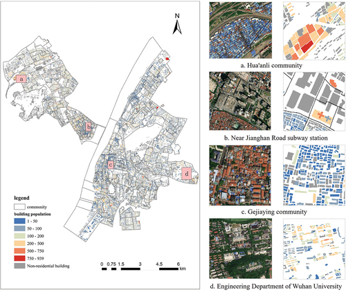
Table 5. Optimal model for estimating the population distribution by district.

Region	Optimal model
Jianghan District	$po{p}_{com}=19.1312{\sum }_{i=0}^{n}E\mathrm{\_}i{n}_i+1084.9561{\sum }_{i=0}^{n}E\mathrm{\_}ou{t}_i$
Wuchang District	$po{p}_{com}=11.8158{\sum }_{i=0}^{n}E\mathrm{\_}i{n}_i+5357.42{\sum }_{i=0}^{n}E\mathrm{\_}ou{t}_i$

In general, the population distribution in the two districts of Wuhan was relatively uniform, mainly because of its polycentric urban functional structure. To further verify the rationality of the DEFF model for estimating the population at the building scale, we visualized the estimated results of the Hu’anli community, vicinity of the Jianghan Road subway station, Gejiaying community, and engineering department of Wuhan University, which represent four typical urban functional areas: urban villages, commercial areas, cultural and educational areas, and general residential areas. Figure 6(a) shows that the population density of the Hu’anli community in Jianghan District is high due to its location near the industrial park, attracting a large number of laborers. The low population living near the subway station in Jianghan District is due to the fact that this area is a large commercial district with most of the buildings being nonresidential and most of the population being distributed among high-rise business residences. However, there are also residential buildings in the lower left corner of Figure 6(b), where the population density is low because this part belongs to the old residential area of Jianghan District, with lower residential floors.

The Gejiaying neighborhood in Wuchang District in Figure 6(c) has a population distribution similar to that of the bottom-left part of Figure 6(b), which is also an older residential area. Wuhan University in Wuchang District houses a large number of faculty, staff, students, and community residents. The population numbers of some of the buildings near its engineering department in Figure 6(d) are significantly higher than those of the surrounding buildings because the population density of these buildings, which are student dormitories, is significantly higher than that of other non-dormitory buildings located nearby.

These visualizations validated the ability of the DEFF to model building-scale population distributions and the necessity of considering the function types of buildings.

4.3. Comparison with other public population datasets

Finding existing works or datasets that are consistent with the extent of our study area and modeling data for comparative analysis remain challenging; therefore, we seek to use general datasets, such as LandScan, WorldPop, and GHS-Pop, for comparative validation, which is also a common evaluation method for population modeling studies (Gui et al. 2022). As shown in Figure 7, compared with the LandScan, WorldPop, and GHS-POP datasets, the proposed DEFF model obtained significantly more accurate building-scale population estimations.

Figure 7. Comparison of the accuracy of various datasets. (a) and (b) Show the comparison of accuracy among our method, LandScan, WorldPop, and GHS-POP at the community level. (c) and (d) Show the comparison of accuracy among our method, LandScan, WorldPop, and GHS-POP at the street level.

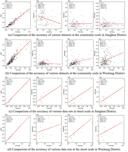
In terms of fitting accuracy, the scattered points obtained with the DEFF model were compact and distributed evenly on both sides of the fitted line. The average fitting accuracy was approximately 78–90% at the community scale and up to 98% at the street scale, which was 60–75% higher than that of existing datasets.

At the community scale, the average values of MAE and RMSE of DEFF decreased by more than 50%, and the average values of MAPE and SMAPE remained stable at 25–30%. At the street scale, the MAE and RMSE values of DEFF decreased by at least 80%, and the MAPE and SMAPE decreased by at least 25% in both Jianghan and Wuchang Districts, thereby demonstrating the validity and stability of our DEFF model.

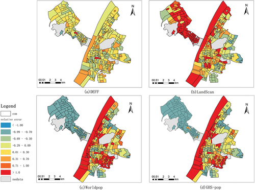
The relative errors of the four datasets were visualized on a community scale. According to the spatial distribution of the relative error shown in Figure 8, the numbers of communities that overestimated and underestimated DEFF were similar, whereas LandScan, WorldPop, and GHS-POP clearly overestimated and underestimated many areas. In the Jianghan and Wuchang districts, LandScan clearly overestimated the number of communities distributed along the Yangtze River. LandScan uses an asymmetric method with a wide range of estimation and coarse-scale features, which could explain the overestimation in urban areas and underestimation in suburban areas. The WorldPop and GHS-POP datasets, which used finer-scale modeling units and features than the LandScan dataset, underestimated the communities in Jianghan District but clearly overestimated the communities distributed along the Yangtze River in Wuchang District. The DEFF model overestimated some university areas because the residential buildings in these areas were dormitory buildings, and the population density was much higher than that in ordinary residential areas. Therefore, the accuracy of the model can be improved by further subdividing the building types.

Figure 8. Comparison of population distribution errors among our method, LandScan, WorldPop, and GHS-POP at the street level.

5. Conclusions and discussion

Building-scale population distribution is important for urban planning and resource allocation. However, most prior studies on building-scale population distribution have only integrated the features of buildings at a single scale (e.g. building scale) and ignored the fact that different spatial features have different optimal representation scales or units. In this study, we propose a method for population estimation based on DEFF. In this method, the internal and external environmental boundaries of buildings were constructed to provide suitable spatial scales for multi-source geographic data feature representation. In addition, we propose a building function-type identification process based on public awareness of POI types to provide effective features for building-scale population modeling. Moreover, the TOPSIS method was improved based on the DQW to yield appropriate fusion weights for external environmental features.

The ablation experiments conducted in this study provided conclusive evidence regarding the soundness and essentiality of each module in our method. In addition, the comparison experiments showed that the results of the DEFF method at the community scale had an $R^2$ of approximately 0.8, an MAE of approximately 1200, an RMSE of approximately 1700, and both MAPE and SMAPE of approximately 26%, indicating better performance than the existing LandScan, WorldPop, and GHS-POP datasets and verifying the validity of our DEFF method for building-scale population estimation.

However, this study has some limitations. The types of residential buildings were not further subdivided, whereas the population densities in residential buildings of types, such as school dormitories, shanty towns, and villages varied widely. In addition, the external environments (i.e. traffic analysis zones) of buildings were constructed from the road network alone, which resulted in large variations in the sizes of the external environments of different buildings, thus amplifying the variation in the external environment features of different buildings and reducing the overall quality of the external environment features. Moreover, it is particularly difficult to obtain multisource spatial data for the same year, which limits the performance of the proposed method. Future research could focus on the following problems: (1) subdividing residential building types to improve the model’s ability to express the differences in population density of different types of residential buildings; (2) considering more factors, such as water networks and areas of interest, when constructing the external environment of the building to reduce the variation in the spatial size of different external environments; and (3) enhancing the application of crowdsourced and open-source data to avoid year inconsistencies in multi-source data.

Disclosure statement

No potential conflict of interest was reported by the authors.

Data availability statement

The data that support the findings of this study are available from the corresponding author, upon reasonable request.

Additional information

Funding

This work is supported by the National Natural Science Foundation of China [Grant numbers U20A2091, 41930107]

Notes on contributors

Guangyu Liu

Guangyu Liu is a master student in the School of Remote Sensing and Information Engineering, Wuhan University. Her research interests are population spatialization and spatiotemporal data analysis.

Rui Li

Rui Li received the M.S. degree in computer application and the PhD degree in communication and information system from Wuhan University, Wuhan, China, in 1999 and 2006, respectively. She is currently a full Professor in the State Key Laboratory of Information Engineering in Surveying, Mapping and Remote Sensing, Wuhan University. Her scientific interests include spatial-temporal computing and big data mining, knowledge graph and semantic computing, web spatial behavior analysis.

Jing Xia

Jing Xia is a PhD student in the State Key Laboratory of Information Engineering in Surveying, Mapping and Remote Sensing, Wuhan University. His research interests are spatial-temporal big data mining and knowledge graphs.

Zhaohui Liu

Zhaohui Liu is a PhD student in the State Key Laboratory of Information Engineering in Surveying, Mapping and Remote Sensing, Wuhan University. His research interests are human mobility analysis and prediction.

Jing Cai

Jing Cai is a PhD student in the State Key Laboratory of Information Engineering in Surveying, Mapping and Remote Sensing, Wuhan University. Her research interests are spatial-temporal data computing and pattern mining.

Huayi Wu

Huayi Wu received the M.S. degree in probability and mathematical statistics and the PhD degree in photogrammetry and remote sensing from Wuhan University, Wuhan, China, in 1991 and 1999, respectively. Is a full Professor in the State Key Laboratory of Information Engineering in Surveying, Mapping and Remote Sensing, Wuhan University. His research interests are high-performance geospatial computing and intelligent geospatial web services.

Mingjun Peng

Mingjun Peng received the M.S. degree in urban planning and the PhD degree in photogrammetry and remote sensing from Wuhan University, Wuhan, China, in 2001 and 2006, respectively. He is a senior engineer in Wuhan Geomatics Institute, and his main research interests are smart city, GIS and spatial-temporal analysis. He has participated in research on some National Key Technologies R&D Program of China, and as the editor of multiple national industry standards.

References

- Balakrishnan, K. 2020. “A Method for Urban Population Density Prediction at 30m Resolution.” Cartography and Geographic Information Science 47 (3): 193–213. https://doi.org/10.1080/15230406.2019.1687014.
- Bright, E., A. Rose, and M. Urban. 2016. LandScan Global 2015. Oak Ridge National Laboratory. https://doi.org/10.48690/1524210.
- Cao, Y., J. Liu, Y. Wang, L. Wang, W. Wu, and F. Su. 2020. “A Study on the Method for Functional Classification of Urban Buildings by Using POI Data.” Journal of Geo-Information Science 22 (6): 1339–1348. https://doi.org/10.12082/dqxxkx.2020.190608.
- Chen, C., A. Qiu, X. Zhao, Y. Zhu, and S. Zhang. 2022. “Urban Functional Area Division Based on AOI Data and Random Forest Method.” Science of Surveying & Mapping 47 (7): 160–168. https://doi.org/10.16251/j.cnki1009-2307.2022.07.021.
- Chen, W., Y. Zhou, and Q. Wu. 2020. “Urban Building Type Mapping Using Geospatial Data: A Case Study of Beijing, China.” Remote Sensing 12 (17): 2805. https://doi.org/10.3390/rs12172805.
- Chen, Z., L. Zhou, W. Yu, L. Wu, and Z. Xie. 2020. “Identification of the Urban Functional Regions Considering the Potential Context of Interest Points.” Acta Geodaetica et Cartographica Sinica 49 (7): 907–920. https://doi.org/10.11947/j.AGCS.2020.20190315.
- Chi, J., L. Jiao, T. Dong, Y. Gu, and Y. Ma. 2016. “Quantitative Identification and Visualization of Urban Functional Area Based on POI Data.” Journal of Geomatics 41 (2): 68–73. https://doi.org/10.14188/j.2095-6045.2016.02.017.
- Dong, N., X. Yang, and H. Cai. 2016. “A Method for Demographic Data Spatialization Based on Residential Space Attributes.” Progress in Geography 35 (11): 1317–1328. https://doi.org/10.18306/dlkxjz.2016.11.002.
- Freire, S., K. MacManus, M. Pesaresi, E. Doxsey-Whitfield, and J. Mills. 2016. “Development of New Open and Free Multi-Temporal Global Population Grids at 250mresolution.” Paper presented at the 19th AGILE Conference on Geographic Information Science, Helsinki, Finland. 250.
- Gui, Z., Y. Mei, H. Wu, and R. Li. 2022. “Urban Population Spatialization by Considering the Heterogeneity on Local Resident Attraction Force of POIs.” Journal of Geo-Information Science 24 (10): 1883–1897. https://doi.org/10.12082/dqxxkx.2022.220384.
- Han, D., X. Yang, H. Cai, X. Xu, Z. Qiao, C. Cheng, N. Dong, D. Huang, and A. Liu. 2019. “Modelling Spatial Distribution of Fine-Scale Populations Based on Residential Properties.” International Journal of Remote Sensing 40 (14): 5287–5300. https://doi.org/10.1080/01431161.2019.1579387.
- He, L., J. Pan, and L. Dong. 2020. “Study on the Spatial Identification of Housing Vacancy.” Remote Sensing Technology and Application 35 (4): 820–831. https://doi.org/10.11873/j.issn.1004-0323.2020.4.0820.
- Hu, Q., R. Li, H. Wu, and Z. Liu. 2022. “Construction of a Refined Population Analysis Unit Based on Urban Forms and Population Aggregation Patterns.” International Journal of Digital Earth 15 (1): 79–107. https://doi.org/10.1080/17538947.2021.2013963.
- Kubíček, P., M. Konečný, Z. Stachoň, J. Shen, L. Herman, T. Řezník, K. Staněk, R. Štampach, and Š. Leitgeb. 2019. “Population distribution modelling at fine spatio-temporal scale based on mobile phone data.” International Journal of Digital Earth 12 (11): 1319–1340. https://doi.org/10.1080/17538947.2018.1548654.
- Lai, Y., T. Liu, and C. Hwang. 1994. “Topsis for MOZDM.” European Journal of Operational Research 76 (3): 486–500. https://doi.org/10.1016/0377-2217(94)90282-8.
- Li, D. and J. Peng. 2007. “Transformation Between Urban Spatial Lnformation Lrregular Grid and Regular Grid.” Geomatics and Information Science of Wuhan University 2007 (2): 95–99. https://doi.org/10.3321/j.issn:1671-8860.2007.02.001.
- Li, S., L. Wang, and N. Dong. 2013. “Simulation of Urban Small-Area Population Space-Time Distribution Based on Building Extraction: Taking Beijing Donghuamen Subdistrict as an Example.” Journal of Geo-Information Science 15 (1): 19–28. https://doi.org/10.3724/SP.J.1047.2013.00019.
- Li, Z., L. Jiao, B. Zhang, G. Xu, and J. Liu. 2021. “Understanding the Pattern and Mechanism of Spatial Concentration of Urban Land Use, Population and Economic Activities: A Case Study in Wuhan, China.” Geo-Spatial Information Science 24 (4): 678–694. https://doi.org/10.1080/10095020.2021.1978276.
- Lin, X., and J. Zhang. 2017. “Object-Based Morphological Building Index for Building Extraction from High Resolution Remote Sensing Lmagery.” Acta Geodaetica et Cartographica Sinica 46 (6): 724–733. https://doi.org/10.11947/j.AGCS.2017.20170068.
- Liu, X., P. Kyriakidis, and M. Goodchild. 2008. “Population Density Estimation Using Regression and Area-To-Point Residual Kriging.” International Journal of Geographical Information Science 22 (4): 431–447. https://doi.org/10.1080/13658810701492225.
- Liu, Z., Z. Gui, H. Wu, K. Qin, J. Wu, Y. Mei, and J. Zhao. 2021. “Fine-Scale Population Spatialization by Synthesizing Building Data and POI Data.” Journal of Geomatics 46 (5): 102–106. https://doi.org/10.14188/j.2095-6045.2019182.
- Lloyd, C. T., H. J. W. Sturrock, D. R. Leasure, W. C. Jochem, A. N. Lázár, and A. J. Tatem. 2020. “Using GIS and Machine Learning to Classify Residential Status of Urban Buildings in Low and Middle Income Settings.” Remote Sensing 12 (23): 3847. https://doi.org/10.3390/rs12233847.
- Loh, W., and Y. Shin. 1997. “Split Selection Methods for Classification Trees.” Statistica Sinica 7 (4): 815–840. https://doi.org/10.1007/s004400050133.
- Lv, A., C. Li, Z. Lin, and Y. Jin. 2002. “Spatial Distribution of Statistical Population Data.” Geomatics and Information Science of Wuhan University 27 (3): 301–305. https://doi.org/10.3969/j.issn.1671-8860.2002.03.014.
- Mei, Y., Z. Gui, J. Wu, D. Peng, R. Li, H. Wu, and Z. Wei. 2022. “Population Spatialization with Pixel-Level Attribute Grading by Considering Scale Mismatch Issue in Regression Modeling.” Geo-Spatial Information Science 25 (3): 365–382. https://doi.org/10.1080/10095020.2021.2021785.
- Meng, Y., R. Li, J. Jiang, S. Wang, and H. Wu. 2021. “Urban Street Scale Population Estimation Based on Building Information.” Geomatics and Information Science of Wuhan University 46 (8): 1194–1200. https://doi.org/10.13203/j.whugis20190343.
- Mennis, J. 2009. “Dasymetric Mapping for Estimating Population in Small Areas.” Geography Compass 3 (2): 727–745. https://doi.org/10.1111/j.1749-8198.2009.00220.x.
- Metzger, N., J. E. Vargas-Muñoz, R. C. Daudt, B. Kellenberger, T. T. Whelan, F. Ofli, M. Imran, K. Schindler, and D. Tuia. 2022. “Fine-Grained Population Mapping from Coarse Census Counts and Open Geodata.” Scientific Reports 12 (1): 20085. https://doi.org/10.1038/s41598-022-24495-w.
- Mileu, N., M. Queirós, and P. Morgado. 2022. “Mapping Population Distribution from Open Address Data: Application to Mainland Portugal.” Journal of Maps 18 (3): 585–593. https://doi.org/10.1080/17445647.2022.2114862.
- Min, Y., Y. Zou, Q. Wang, and P. Rao. 2019. “Study of Urban Population Spatial Distribution Based on CA/MAS.” Modern Surveying and Mapping 42 (2): 7–12. https://doi.org/10.3969/j.issn.1672-4097.2019.02.002.
- Shang, S., S. Du, S. Du, and S. Zhu. 2021. “Estimating building-scale population using multi-source spatial data.” Cities 111:103002. https://doi.org/10.1016/j.cities.2020.103002.
- Wang, L., L. Wang, and M. Cai. 2022. “Research on Dynamic Weight Fusion Method Based on Multi-Source Speed data.B2022.” Acta Scientiarum Naturalium Universitatis Sunyatseni 61 (5): 31–40. https://doi.org/10.13471/j.cnki.acta.snus.2021B019.
- Wang, M., Y. Wang, B. Li, Z. Cai, and M. Kang. 2022. “A Population Spatialization Model at the Building Scale Using Random Forest.” Remote Sensing 14 (8): 1811. https://doi.org/10.3390/rs14081811.
- Wang, S., R. Li, J. Jiang, and M. Yao. 2021. “Fine-Scale Population Estimation Based on Building Classifications: A Case Study in Wuhan.” Future Internet 13 (10): 251. https://doi.org/10.3390/fi13100251.
- Xia, L., X. Zhang, J. Zhang, H. Yang, and T. Chen. 2021. “Building Extraction from Very-High-Resolution Remote Sensing Images Using Semi-Supervised Semantic Edge Detection.” Remote Sensing 13 (11): 2187–2187. https://doi.org/10.3390/RS13112187.
- Yang, X., Z. Fang, and L. Yin. 2018. “Exploring the Relationship Between Urban Spatial Structure and the Stability of Human Convergence-Divergence.” Journal of Geo-Information Science 20 (6): 791–798. https://doi.org/10.12082/dqxxkx.2018.180026.
- Yao, Y., X. Liu, X. Li, J. Zhang, Z. Liang, K. Mai, and Y. Zhang. 2017. “Mapping Fine-Scale Population Distributions at the Building Level by Integrating Multisource Geospatial Big Data.” International Journal of Geographical Information Science 31 (6): 25. https://doi.org/10.1080/13658816.2017.1290252.
- Zhang, D., D. Li, L. Zhou, J. Huang, G. Hang, J. Wang, and Y. Ma. 2021. “High Precision Space Estimation of Housing Vacancy Rate Using High Resolution Image and Luojia-1.” Bulletin of Surveying & Mapping 1:41–46+52. https://doi.org/10.13474/j.cnki.11-2246.2021.0008.
- Zhang, G., S. Poslad, Y. Fan, and X. Rui. 2022. “Quantitative Spatiotemporal Impact of Dynamic Population Density Changes on the COVID-19 Pandemic in China’s Mainland.” Geo-Spatial Information Science 1–22. https://doi.org/10.1080/10095020.2022.2066576.
- Zhao, W., Q. Li, and B. Li. 2011. “Extracting Hierarchical Landmarks from Urban POI Data.” Journal of Remote Sensing 15 (5): 973–988. https://doi.org/10.11834/jrs.20110173.
- Zhao, Y., Q. Li, Y. Zhang, and X. Du. 2019. “Improving the Accuracy of Fine-Grained Population Mapping Using Population-Sensitive POIs.” Remote Sensing 11 (21): 2502. https://doi.org/10.3390/rs11212502.