Analysis of wave breaking on synthetic aperture radar at C-band during tropical cyclones

ABSTRACT

The purpose of our work is to analyze the effect of wave breaking on dual-polarized (vertical-vertical (VV) and vertical-horizontal (VH)) synthetic aperture radar (SAR) image in the C-band during tropical cyclones (TCs) based on the machine learning method. In this study, more than 1300 Sentinel-1 (S-1) interferometric-wide (IW) and extra wide (EW) mode SAR images are collocated with wave simulations from the WAVEWATCH-III (WW3) model during 400 TCs. The validation of the significant wave height (SWH) simulated using the WW3 model against Jason-2 altimeter data. The winds for S-1 SAR images are reconstructed using wind retrievals in VV and VH polarization. The non-polarized (NP) contribution σ_wb caused by wave breaking is assumed to be the result of the SAR-measured normalized radar cross-section (NRCS) σ₀ minus the Bragg resonant roughness σ_br without the distortion of rain cells during TCs. The σ_br is simulated by imputing wave spectra from the WW3 model into the theoretical backscattering model. It is found that the ratio (σ_wb/σ₀) in VV polarization is related to the wind speed, the wind direction relative with the flight orientation, and radar incidence angle. Following this rationale, the Adaptive Boosting (AdaBoost) model was used for the estimation of NP contribution σ_wb during TCs and are implemented for more than 300 dual-polarized S-1 images to validate the model. It is found that for the comparison between the sum of simulation NRCS and SAR observations, the root mean squared error (RMSE) is 1.95 dB and the coefficient (COR) is 0.86, which is better than a 2.83 dB RMSE and a 0.67 COR by empirical model. It is concluded that the AdaBoost model has a good performance on NP component simulation during TCs.

KEYWORDS:

• Wave breaking
• synthetic aperture radar
• tropical cyclone

1. Introduction

Wave breaking is a common phenomenon in wave research (Hanson and Phillips 1999), especially during tropical cyclones (TCs). Under the effect of the wind, wave breaking is generated, due to that wave particles are moved faster than wave maintains and flies upwards. The wave breaking causes whitecap that is the first stage of the wave breaking at 7–8 m/s of wind speed, bubbles, and currents, which promote energy exchange in the sea–air interface layer (Terray et al. 1996). In the last several decades, the wave breaking parameterization has been well researched in the numerical wave models, i.e. the third-generation WAVEWATCH-III (WW3) (Tolman and Chalikov 1996) and simulating wave nearshore (SWAN) models (Akpınar et al. 2012; Yang et al. 2020). However, the numerical models only provide the simulation data and the difficulty in measuring the in-situ data of the wave breaking events, especially in the TCs. Synthetic aperture radar (SAR) is an advanced remote sensing technique for sea surface detection with large swath coverage under all conditions of time and weather (Li 2015), i.e. wind (Shao et al. 2021), wave (Shao et al. 2022), oceanic front (Xie, Perrie, and Chen 2010), and mesoscale eddies (Xu et al. 2015).

At present, the geophysical model function (GMF) is frequently used for SAR wind retrieval. It is based on the normalized radar cross section (NRCS), wind vector, and incidence angle (Yao et al. 2022). In recent studies, SAR-based GMFs in co-polarization (vertical-vertical (VV) and horizontal-horizontal (HH)) have been well developed under low-to-moderate wind conditions, i.e. CMOD5 (Hersbach, Stoffelen, and Haan 2007), CMOD7 (Stoffelen et al. 2017), C-SARMOD (Mouche and Chapron 2016), and CSARMOD-GF (Shao et al. 2021). However, the co-polarized SAR-measured NRCS encounters a saturation problem in high winds (Fernandez et al. 2006), indicating that the co-polarized SAR GMF (Hersbach 2010) is not suitable for cyclonic wind retrieval. Recent studies have revealed (Hwang et al. 2015) that high winds can be directly retrieved from cross-polarized (vertical-horizontal (VH) and horizontal-vertical (HV)) SAR-measured NRCS using an empirical model (Shao et al. 2018), such as the C-band cross-polarization ocean (C-3PO) for RADARSAT-2 (R-2) and the Sentinel-1 (S-1) interferometric-wide/extra wide (EW) (IW/EW) mode wind speed retrieval model after noise removal (S1IW.NR/S1EW.NR) (Gao et al. 2021; Zhao et al. 2023). Although the method of retrieving the TC wind from the cross-polarization NRCS from SAR is reliable (Hwang et al. 2015), the ocean phenomena during TC processes disturbs the SAR backscattering signal from the ocean surface, resulting in the distortion of the TC SAR wind retrieval.

Existing SAR wave algorithms can be divided into two basic classical approaches: 1) transfer function-based scheme, which converts the image spectrum into a wave spectrum with a subsequent estimation of the integrated sea state parameters (Alpers and Bruning 1986; Hu et al. 2023), i.e. the Max Planck Institute algorithm (Hasselmann and Hasselmann 1991; Hasselmann et al. 1996), the partition rescaling and shift algorithm (Schulz-Stellenfleth, Lehner, and Hoja 2005), and the parameterized first-guess spectrum method (Jiang et al. 2023; Lin et al. 2017); 2) empirical models which estimate the sea state parameters directly from features derived from the SAR scene. The first generation of empirical models is derived from simple empirical functions through NRCS and azimuthal cutoff wave length (i.e. Bao et al. 2022; Bruck 2015). The second generation of empirical models are based on linear regression approach for C-band SARs (Schulz-Stellenfleth, Konig, and Lehner 2007; Sheng et al. 2018) and TerraSAR-X (TS-X) (Pleskachevsky, Rosenthal, and Lehner 2016; Shao et al. 2020). Recently, the third generation of the wave retrieval algorithm is improved by the deep learning (Pleskachevsky et al. 2022; Quach et al. 2020; Wang et al. 2022), i.e. 25 cm accuracy of significant wave height (SWH) for Sentinel-1 (S-1) wave mode (WV). In addition, the full polarimetric technique can be applied for SAR wave retrieval only considering tilt modulation (He, Shen, and Perrie 2006). In a previous study (Zhong et al. 2023), the breaking waves were found to have an impact on the wave retrieval algorithm for Gaofen-3 and TS-X images under low and moderate sea states. The whitecaps produced by wave breaking change the orientation normal to the facet of the long wave, which can reduce the effect of the tilt modulation on the SAR. Therefore, SAR wind and wave retrieval should consider the influence of breaking waves, especially during TCs.

In previous studies, SAR backscattering is mainly produced via two aspects: resonant Bragg components determined by wind-induced waves and the non-polarized (NP) component induced by breaking waves (Hwang, Zhang, and Perrie 2010; Sun et al. 2022) and other atmospheric and marine processes such as rainfall (Melsheimer, Alpers, and Gade 2001). The breaking waves affect the surface roughness and the homogeneity of co-polarized SAR backscattering signals (Hwang and Fois 2015), resulting in difficulty in SAR wave retrieval under high sea states. In previous studies, polarimetric SAR data have been used to study the effect of breaking waves on the modeling of quad-polarization radar scattering (Wang et al. 2022; Zhang et al. 2020) and the co-polarized and cross-polarized radar return (Kudryavtsev et al. 2013). The empirical relationship between the wave breaking effect on the cross-polarization return and the total energy dissipation rate proposed by Hwang et al. (2010) was applied to improve the hurricane wind retrieval method on the dual and quad-polarimetric R-2 SAR images. Furthermore, utilizing polarimetric R-2 SAR images collocated with the measurements from moored buoys, the NP contribution of breaking waves in radar backscattering signals, denoted as the NRCS, was estimated and an empirical function was reconstructed (Kudryavtsev et al. 2019), but it only considered wind speeds under low-to-moderate sea states. Wave breaking during TCs has additional significance in air – sea interactions and energy exchange. Up to now, analysis of wave breaking on SAR during TCs has not been sufficiently conducted, therefore, the characteristics of the impact of the NP component on SAR based on machine learning method is worthy of comprehensive study through ambulant dataset (> images) (i.e. Pleskachevsky et al. 2022).

A theory-based approach has been used to calculate the contribution of the NP component from TerraSAR-X and Gaofen-3 images using both VV-polarized and HH-polarized SAR-measured NRCS (Sun et al. 2022; Viana et al. 2020; Zhong et al. 2023). However, this approach is not applicable for dual-polarized (VV and VH) SAR. Therefore, in this study, the contribution of the NP component is calculated as the difference between the simulated Bragg resonant component and the SAR observations (Morten et al. 2016). The Bragg resonant component in the NRCS is calculated using a backscattering model, which relies on the SAR-derived wind speed from SAR TC images, the hybrid coordinate ocean model (HYCOM) sea surface currents, and the wave parameters from the WW3 model. In this study, we investigate the impact of wave breaking on C-band SAR using more than 1300 S-1 images acquired in IW and EW mode during TCs. The remainder of this paper is organized as follows. The available datasets are introduced in Section 2. The methodology for estimating the Bragg resonant component in the NRCS and the scheme of a machine learning, denoted as Adaptive Boosting (AdaBoost), is presented in Section 3. The results, including the machine learning method for calculating the NP component and the validation using more than 300 S-1 images, are presented in Section 4. The conclusions are summarized in Section 5.

2. Dataset

The dataset used in this study is grouped into two parts, i.e. dual-polarized SAR images and hindcasting waves from numeric model. In particular, the TC winds are reconstructed based on VV-polarized and VH-polarized SAR-derived winds.

2.1. SAR data

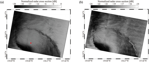
In total, we used more than 1300 S-1 SAR images in dual-polarization (VV and VH) acquired during TCs in this study. These images were taken over global seas during 2015–2022. Here, 1000 S-1 images were used to train the AdaBoost and the other S-1 images were used for validation. These SAR images are open accessed by European Space Agency, in particular, some corrections have been conducted so as to enhance the usability of SAR data, i.e. the removal of the low-intensity GRD border noise, thermal noise removal, radiometric calibration, and refined lee filtering (Shao et al. 2023; Yu et al. 2019). The pixel size of the S-1 images is 10 m in both the azimuth and range directions, with a swath coverage of approximately 200 km and incidence angles of 30.7–46.1°. The whole image is further divided into several sub-scenes with 256 × 256 pixel, meaning that SAR-derived winds are averaged to a spatial resolution of 3 km. Their geographic locations are shown in Figure 1. The black and blue rectangles denote the geographic locations of the S-1 SAR images in training and validation datasets. As an example, Figure 2 presents a VV-polarized and VH-polarized S-1 SAR image during Hurricane Lester at 16:30 UTC on 4 September 2016.

Figure 1. Geographic locations of the collected Sentinel-1 synthetic aperture radar (SAR) images acquired during tropical cyclones (TCs) in 2015–2022, in which the black and blue rectangles represent the spatial coverage of S-1 images in the training and validation datasets, respectively.

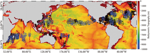
Figure 2. Quick-look of the normalized radar cross-section (NRCS) from the Sentinel-1 (S-1) image acquired in interferometric-wide (IW) swath mode during Hurricane Lester at 16:30 UTC on 4 September 2016 (a) VV-polarized and (b) VH-polarized.

2.2 Wind speed retrieval from SAR

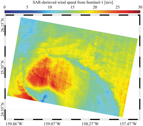
The sea surface wind speed is an important sea surface parameter for simulating the Bragg resonant component in the NRCS. Under typhoon conditions, the method of obtaining the SAR-derived wind speed from S-1 SAR images has been well studied (Gao et al. 2021). As was reported by Melsheimer et al. (2001), it is known that rain cells influence SAR backscattering signals. A recent study (Shao et al. 2022) has proposed a method for the identification of rain cells in S-1 SAR. In particular, the TC wind profiles are reconstructed based on VV-polarized and VH-polarized SAR-derived winds, which improves the discontinuity of the VH-polarized retrieval winds and removes the distortion of the rain cells. Therefore, the above TC wind reconstruction method is used to achieve TC wind retrieval from S-1 SAR images in this paper.

The root mean square error (RMSE) between the TC wind speed retrieval and the stepped-frequency microwave radiometer (SFMR) measurements for the S-1 SAR image is about 4 m/s (Shao et al. 2022). Therefore, the validation of the wind speed retrieval from the TC SAR images is not repeated in this paper. The corresponding SAR-derived wind speed maps with a spatial resolution of approximately 3 km from the S-1 images in Figure 2 are shown in Figure 3.

Figure 3. Corresponding wind retrieval maps from S-1 image during Hurricane Lester at 16:30 UTC on 4 September 2016.

2.3 Hindcast wave from WW3

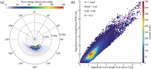
In this paper, these images are collocated with hindcast waves simulated from the WW3 model (Hu et al. 2023; Sheng et al. 2019). The winds from the European Center for Medium-Range Weather Forecasts reanalysis (ERA-5) with a 0.25° grid at intervals of 1 h and currents from the HYCOM with a 1/12° grid at 3 h intervals are used as the forcing field. The water depths are derived from the General Bathymetry Chart of the Oceans with a spatial resolution of approximately 1 km. As an example, Figure 4(a) shows the footprints of the Jason-2 measurements from 1 September 2016 to 10 September 2016. Figure 4(b) presents the SWH map at 16:30 UTC on 4 September 2016, in which the black rectangle corresponds to the geographic location of the image in Figure 2(a). Figure 5(a) shows a two-dimensional wave spectrum from WW3 at the geographic location highlighted by the red dot in Figure 2(a). We use the WW3-simulated SWH collocated with measurements from altimeter Jason-2 for the period from 20 August to 14 September 2016 during Hurricanes Hermine in the region of (255–295°E, 10–45°N), Hurricane Lester in the region of (185–215°E, 10–45°N), and Hurricane Lionrock in the region of (120–160°E, 10–45°N); from 1 September to 20 September 2017 during Hurricane Irma in the region of (270–310°E, 5°–40°N); and from 1 September to 28 September 2017 during Hurricane Maria in the region of (275–315°E, 5–35°N). The validation of the WW3-simulated SWH is shown in Figure 5(b). Comparison of the measurements from the Jason-2 altimeter yields an RMSE of 0.48 m for the SWH, a correlation (COR) of 0.88, and a scatter index (SI) of 0.22, in which the SWHs are grouped into 0.07 m bins. The statistical analysis indicates that the wave simulation from the WW3 model is reliable in this study.

Figure 4. (a) Footprints of the Jason-2 measurements from 1 September 2016 to 10 September 2016; (b) the Significant Wave Height (SWH) map from WW3 for 16:30 UTC on 4 September 2016, in which the black rectangle corresponds to the geographic location of the image in Figure 2(a).

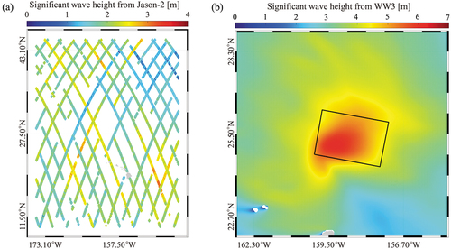
Figure 5. (a) Two-dimensional wave spectrum from the WAVEWATCH-III (WW3) model at the geographic location highlighted by the red dot in Figure 1(a). (b) validation of WW3-simulated Significant Wave Height (SWH) against the measurements from the Jason-2 altimeter, in which the SWHs are grouped into 0.07 m bins.

3. Methodology

In this section, the Bragg backscattering component simulation model is briefly described. Then, an empirical function for calculating the contribution of the NP to the SAR is introduced (Kudryavtsev et al. 2019). Furthermore, the machine learning method, denoted as Adaboost, is presented.

3.1. Bragg backscattering component simulation model

In principle, the contribution of the NP component of the breaking waves (σ_wb) is the difference between the observed NRCS σ₀ and the Bragg backscattering component σ_br without the distortion of rain cells during a TC, that is, σ_wb = σ₀–σ_br. According to backscattering theory, σ_br is directly related to the distribution of the Bragg wave (Kudryavtsev et al. 2003):

(1) ${\sigma }_{br}^{PP}=8\pi k_0^4{cos}^4\theta {\left|{\mathrm{G}}_{PP}\left(\theta ,\epsilon \right)\right|}^2\left[W\left({\vec{\mathit{k}}}_b\right)W\left(-{\vec{\mathit{k}}}_b\right)\right]$(1)

where

(2) $G_{VV}\left(\theta ,\epsilon \right)=\mathrm{c}\mathrm{o}{\mathrm{s}}^2\theta \frac{\left(\epsilon -1\right)[\epsilon \left(1+\mathrm{s}\mathrm{i}{\mathrm{n}}^2\theta \right)-\mathrm{s}\mathrm{i}{\mathrm{n}}^2\theta ]}{{[\epsilon \mathrm{c}\mathrm{o}\mathrm{s}\theta +\sqrt{\epsilon -\mathrm{s}\mathrm{i}{\mathrm{n}}^2\theta }]}^2}$(2)

(3) ${\mathrm{G}}_{\mathrm{H}\mathrm{H}}\left(\theta ,\epsilon \right)=\mathrm{c}\mathrm{o}{\mathrm{s}}^2\theta \frac{\left(\epsilon -1\right)}{{[\mathrm{c}\mathrm{o}\mathrm{s}\theta +\sqrt{\epsilon -\mathrm{s}\mathrm{i}{\mathrm{n}}^2\theta }]}^2}$(3)

In Equations (1)(1) ${\sigma }_{br}^{PP}=8\pi k_0^4{cos}^4\theta {\left|{\mathrm{G}}_{PP}\left(\theta ,\epsilon \right)\right|}^2\left[W\left({\vec{\mathit{k}}}_b\right)W\left(-{\vec{\mathit{k}}}_b\right)\right]$(1) –(3(3) ${\mathrm{G}}_{\mathrm{H}\mathrm{H}}\left(\theta ,\epsilon \right)=\mathrm{c}\mathrm{o}{\mathrm{s}}^2\theta \frac{\left(\epsilon -1\right)}{{[\mathrm{c}\mathrm{o}\mathrm{s}\theta +\sqrt{\epsilon -\mathrm{s}\mathrm{i}{\mathrm{n}}^2\theta }]}^2}$(3) ), pp denotes the either VV or HH polarization, W(${\vec{\mathit{k}}}_b$) is the spectrum of the sea surface waves on the scale of the Bragg component ${\vec{\mathit{k}}}_b$, k₀ is the wave number of the radar beam, ε is the permittivity of sea water, and θ is the radar incidence angle. For large-scale waves, the main factors considered are the tilt modulation and hydrodynamics modulation. Thus, a linear model is adopted to simulate the sea surface. The Bragg scattering coefficient ${\sigma }_{br}$ can be written as

(4) ${\sigma }_{br}=(1+m){\sigma }_{br}^{PP}$(4)

(5) $m\left(x,y,t\right)={\sum }_{k_x}{\sum }_{k_y}T\left(k_x,k_y\right)\varsigma exp[j(k_{x}x+k_{y}y\omega t)]\sqrt{2d{k}_x{k}_y}$(5)

where ω and t are the wave frequency and time, respectively, and T(k_x,k_y) is the sum of the tilt modulation T_t and hydrodynamic modulation T_h in the wave number component terms k_x and k_y in the range (x) and azimuth (y) directions. ς is the wave height spectrum from WW3 mode, which is related to the wave spectrum W as follows:

(6) $⟨\varsigma \left(k_x,k_y\right){\varsigma }^{\ast }\left(k_x,k_y\right)⟩=W\left(k_x,k_y\right)$(6)

(7) $T(k_x,k_y)=T_t+T_h$(7)

(8) $T_t=\frac{4ik{ }^x\mathrm{c}\mathrm{o}\mathrm{t}\theta }{1\pm \mathrm{s}\mathrm{i}{\mathrm{n}}^2\theta }$(8)

(9) $T{ }_h=4.5\left|k_y\right|\omega \frac{\omega -j\mu }{{\omega }^2+{\mu }^2}{cos}^2\left({\vec{\mathit{k}}}_x,{\vec{\mathit{k}}}_y\right)$(9)

in which, $\mu$ is the relaxation rate and ω is the wave frequency.

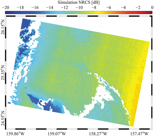
As an example, the Bragg backscattering component NRCS map simulated using the above method, which corresponds to the SAR image in Figure 2(a), is shown in Figure 6, in which the gaps are identified as rain cells.

Figure 6. Simulated NRCS map corresponding to the SAR image in Figure 2(a), in which the gaps are identified as rain cells.

3.2. Empirical function for calculating the contribution of the NP component

A practical function for the estimation of σ_wb has recently been developed, using the following formulation (Kudryavtsev et al. 2019):

(10) ${\sigma }_{wb}=F(\theta )Y(\varphi )U_{10}^{B(\theta )}$(10)

where

(11) $F(\theta )=0.00019e^{-0.32\times (\theta -{30}^{°})}$(11)

(12) $B(\theta )=1.3+0.047\times (\theta -{30}^{°})$(12)

(13) $Y(\theta )=exp(a_0+a_1\mathrm{c}\mathrm{o}\mathrm{s}\varphi +a_2\mathrm{c}\mathrm{o}\mathrm{s}2\varphi )$(13)

(14) $a_0=0.24-0.014\times (\theta -{30}^{\circ })$(14)

(15) $a_1=0.33+0.013\times (\theta -{30}^{\circ })$(15)

(16) $a_2=0.12+0.014\times (\theta -{30}^{\circ })$(16)

Although the above equations, which require the radar incidence angle θ, the azimuth angle $\varphi$, and the sea surface wind speed at a height of 10 m U₁₀, are convenient to apply, they are not valid under extreme conditions because the functions F(θ), Y($\varphi$), and B(θ) are fitted at low-to-moderate wind speeds.

3.3. AdaBoost

AdaBoost is a powerful ensemble learning algorithm tailed to combine multiple weak classifiers to create one strong classifier. It gradually improves the performance of the overall model by adjusting sample weights, in which previously misclassified samples receive more attention. The core steps of AdaBoost model follows three steps.

(1) For a dataset containing N training samples, the initial weights for each sample are initialized to uniform values (= 1/N). The initial weight formula is shown in Equation (17)(17) $w_i^{(1)}=\frac{1}{N},i=1,2,\dots ,N$(17)

(17) $w_i^{(1)}=\frac{1}{N},i=1,2,\dots ,N$(17)

(2) For each iteration t, train a weak classifier $h_t$ by minimizing the weighted classification error rate, which has better performance under the current sample weight. And then, the weight of the weak classifier ${\alpha }_t$ is calculated from its classification error rate ${\epsilon }_t$, which is defined as the ratio of the total weight of the misclassified samples to the weight of all samples. The weight calculation formula of weak classifier is present in Equation (18)(18) ${\alpha }_t=\frac{1}{2}\mathrm{l}\mathrm{n}\left(\frac{1-{\epsilon }_t}{{\epsilon }_t}\right)$(18) :

(18) ${\alpha }_t=\frac{1}{2}\mathrm{l}\mathrm{n}\left(\frac{1-{\epsilon }_t}{{\epsilon }_t}\right)$(18)

Using the Equations (19)(19) $w_i^{(t+\text{1})}=w_i^{(t)}\cdot exp(-{\alpha }_{\mathrm{t}})$(19) and (20(20) $w_i^{(t+\text{1})}=w_i^{(t)}\cdot exp({\alpha }_{\mathrm{t}})$(20) ) to adjust the weights of the correctly classified and misclassified samples. So, the weights of the misclassified samples increase. In the next iteration, the model focuses on the misclassified samples and reduces the weights of the correctly classified samples to update sample weights.

(19) $w_i^{(t+\text{1})}=w_i^{(t)}\cdot exp(-{\alpha }_{\mathrm{t}})$(19)

(20) $w_i^{(t+\text{1})}=w_i^{(t)}\cdot exp({\alpha }_{\mathrm{t}})$(20)

(3) After the iterative process, the final strong classifier by weighted summing the output of each weak classifier was built. The strong classifier formula was as follows:

(21) $H(x)=\sum _{t=1}^T{\alpha }_t{h}_t\left(x\right)$(21)

where T is the total number of iterations, ${\alpha }_t$ is the weight of the t-th weak classifier, and $h_t(x)$ is the output of the t-th weak classifier. Finally, the classification prediction of new samples using the constructed strong classifier. Figure 7 shows the scheme of the AdaBoost model.

Figure 7. The scheme of the AdaBoost model.

4. Results and discussion

The dependence of parameters on NP component in NRCS is firstly presented. Based on the finding, the AdaBoost machine learning for simulating NP component in NRCS was training and the validation of the AdaBoost model is discussed here.

4.1 Machine learning method for calculating the NP component

The regions without rain cells are used to calculate the NP component in the NRCS σ_wb associated with wave breaking. The σ_wb ratio in the VV-polarized ${\sigma }_0^{\mathrm{v}\mathrm{v}}$NRCS are calculated. The S-1 images are divided into 128 × 128 pixel sub-scenes, with a spatial coverage of 3 km. The sub-scenes are used to estimate the rain cells, SAR-derived wind speed, incidence angle, azimuth angle, and wind direction. There were more than one million samples collocated with the ${\sigma }_{wb}/{\sigma }_0^{\mathrm{v}\mathrm{v}}$ ratio, incidence angle, azimuth angle, wind direction, and wind speed from the S-1 image, which is treated as the training dataset. 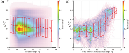Figure 8 shows the results of the ${\sigma }_{wb}/{\sigma }_0^{\mathrm{v}\mathrm{v}}$ ratio with respect to the SAR-derived wind speed. It is found that the ratio linearly increases with increasing wind speed. Because wave breaking is determined by the wave state, the VV-polarized ratio has no saturation problem under strong winds. Figure 9(a,b) show the relationship between the ${\sigma }_{wb}/{\sigma }_0^{\mathrm{v}\mathrm{v}}$ ratio and the incidence angle and the relationship between the ${\sigma }_{wb}/{\sigma }_0^{\mathrm{v}\mathrm{v}}$ ratio and the wind direction minus the azimuth angle, respectively. The ratio decreases with increasing incidence angle, which is consistent with the conclusion of Sun et al. (2022). The ratio decreases when the relative wind direction is <60°, and the ratio increases when the relative wind direction is >60°. The ratio is related to the incidence angle and the bias (wind direction minus the azimuth angle).

Figure 8. Relationship between the ${\sigma }_{wb}/{\sigma }_0^{\mathrm{v}\mathrm{v}}$ ratio and the SAR-derived wind speed U₁₀. The red line is the error bar of the ratio. The blue line is the fitting curve for the data.

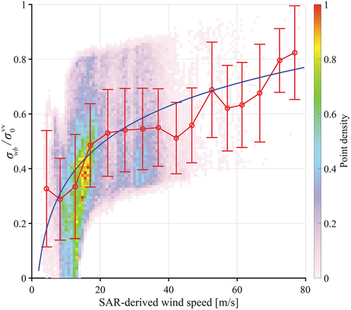
Figure 9. Relationship between the ${\sigma }_{wb}/{\sigma }_0^{\mathrm{v}\mathrm{v}}$ ratio and the (a) incidence angle θ and (b) wind direction minus the azimuth angle ϕ.

Based on the above findings, the AdaBoost model was used for estimating the NP component during a TC from the one hundred S-1 images. 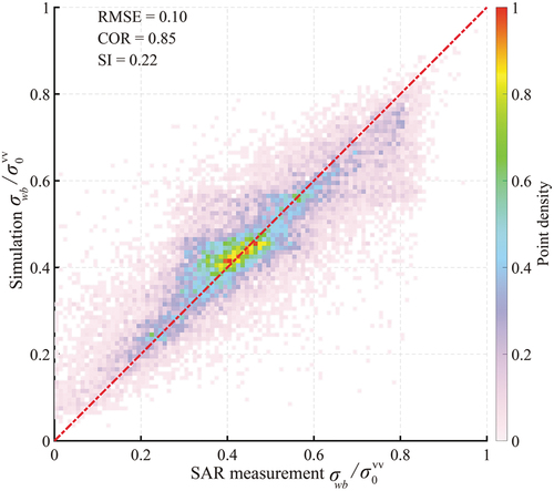In the training procedure, the input parameters contain, U₁₀ is the wind speed at a height 10 m of above the sea surface, θ is the incidence angle, and φ is the wind direction relative to the azimuth angle, and the output is the ${\sigma }_{wb}/{\sigma }_0^{\mathrm{v}\mathrm{v}}$ ratio, in which σ_wb is the NP component, ${\sigma }_0^{\mathrm{v}\mathrm{v}}$ is the observed NRCS in VV polarization. Figure 10 shows the performance of the AdaBoost training process. It is observed that the machine learning will eventually converge and the decision coefficient (R-squared) achieved is close to 0.88. Figure 11 shows the comparison results between the ${\sigma }_{wb}/{\sigma }_0^{\mathrm{v}\mathrm{v}}$ ratio simulated using the AdaBoost model and the values from the S-1 images, which yields an RMSE of 0.10, an SI of 0.22, and a COR of 0.85. Thus, we conclude that the AdaBoost for estimating the NP component can be applied to VV-polarized SAR images acquired during TCs.

Figure 10. The performance of the AdaBoost model training process.

Figure 11. The ${\sigma }_{wb}/{\sigma }_0^{\mathrm{v}\mathrm{v}}$ ratio from the S-1 images versus the simulated values obtained using the proposed empirical model.

4.2 Validation and discussion of the proposed model

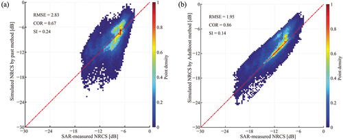
In addition, more than 300 dual-polarized S-1 images acquired in IW mode and EW mode was used to validate the AdaBoost. The Bragg component in the NRCS is simulated using the WW3-simulated wave spectrum and the NP component is calculated using Equation (10)(10) ${\sigma }_{wb}=F(\theta )Y(\varphi )U_{10}^{B(\theta )}$(10) and the proposed model. More than 120,000 samples are collocated on the S-1 images for validation analysis. Figure 12(a) depicts the NRCS map from the S-1 image during Hurricane Lester at 16:30 UTC on 4 September 2016, with the average of 256 × 256 pixels (approximately 3 km). Figure 12(b) presents the composite NRCS map of the Bragg resonant and NP component obtained using the AdaBoost, in which the gaps are identified as rain cells. Although the NRCS map obtained using the AdaBoost is larger than the SAR-measurements in some areas, the two NRCS maps have consistent space distributions. A comparison of the sum of the simulation NRCS and SAR observations is shown in Figure 13, i.e. the result obtained using Equation (10)(10) ${\sigma }_{wb}=F(\theta )Y(\varphi )U_{10}^{B(\theta )}$(10) (Figure 13(a)) and the AdaBoost (Figure 13(b)). The AdaBoost yields an RMSE of 1.95 dB and a COR of 0.86, which is better than those (RMSE of 2.83 dB and COR of 0.67) obtained using Equation (10)(10) ${\sigma }_{wb}=F(\theta )Y(\varphi )U_{10}^{B(\theta )}$(10) . Therefore, the proposed empirical model is suitable for estimating the NP component during TCs.

Figure 12. (a) The NRCS map from the VV-polarized S-1 image during hurricane Lester at 16:30 UTC on 4 September 2016, with the average of 256 × 256 pixels; and (b) the composite NRCS map of the Bragg resonant and NP component obtained using the AdaBoost, in which the gaps are identified as rain cells.

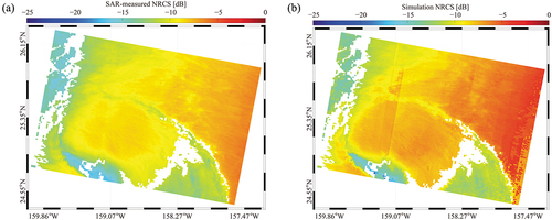
Figure 13. Comparison of the S-1 SAR-measured NRCSs and the values simulated using (a) Equation (10)(10) ${\sigma }_{wb}=F(\theta )Y(\varphi )U_{10}^{B(\theta )}$(10) and (b) the AdaBoost model.

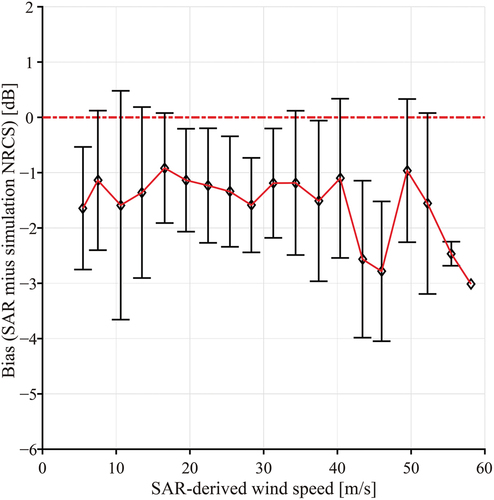
The difference in the NRCS (SAR observations minus simulation) with respect to the wind speed for a 3 m/s bin is presented in Figure 14. The difference in the NRCS is a negative number when the wind speed increases. The whitecaps produced by wave breaking change the sea surface, which could enhance the specular reflection to the SAR backscattering signal, resulting in overestimation of the AdaBoost. Furthermore, the difference in the NRCS remains to within −2 dB when the wind speed is smaller than 40 m/s. The difference in the NRCS likely increases when the wind speed is greater than 40 m/s, indicating that the accuracy of the proposed model decreases with increasing winds. The large error is probably caused by the inaccuracy of the SAR-derived strong wind.

Figure 14. The difference in the NRCS (SAR observation minus simulation) with respect to the wind speed for a 3 m/s bin. The error-bars represent the standard deviations of the bins.

5. Conclusions

The advantage of SAR is its ability to monitor sea surface dynamics with a fine spatial resolution and large swath coverage (Shao et al. 2022). In particular, SAR is capable of retrieving wind and wave fields during TCs. Strong wind-induced wave breaking is an essential dynamic process at the air-sea layer. In this study, the impact of the NP component of wave breaking on the C-band SAR backscattering signal during TCs was investigated, and then a machine learning method for estimating the contribution of the NP component was developed.

In our work, more than 1300 dual-polarized S-1 images were collocated with WW3 model simulations during 400 TCs. TC wind profiles were reconstructed using wind retrievals in VV and VH polarization so as to remove the influence of SAR artifacts (Shao et al. 2023) for S-1. The Bragg resonant component in the NRCS, σ_br, was simulated using a backscattering model and WW3-simulated wave spectra. Then, to obtain the NP component, we subtracted σ_br from the observed NRCS σ₀ from the VV-polarized SAR images (σ_wb = σ₀ – σ_br) in regions without the distortion of rain cells. It was found that the ${\sigma }_{wb}/{\sigma }_0^{\mathrm{v}\mathrm{v}}$ ratio is related to the wind speed and the wind direction relative to flight orientation, and the ${\sigma }_{wb}/{\sigma }_0^{\mathrm{v}\mathrm{v}}$ ratio decreases with increasing incidence angle. Based on the findings, a machine learning method, called AdaBoost, was used for estimating σ_wb from S-1 during TCs. Moreover, this model was validated through application to more than 300 dual-polarized S-1 images and comparison with the practical function derived by Kudryavtsev et al. (2019). The proposed model yielded an RMSE of 1.95 dB and a COR of 0.86, which are better than those (RMSE of 2.83 dB and COR of 0.67) obtained using Equation (10)(10) ${\sigma }_{wb}=F(\theta )Y(\varphi )U_{10}^{B(\theta )}$(10) . Relative to the physical and empirical models of NP component (Kudryavtsev et al. 2019; Morten et al. 2016), the proposed AdaBoost is suitable for estimating the NP component during TCs. In the near future, more SAR images in the C-band will be collected during the hurricane season. In addition, because wave breaking has a significant influence on the SAR roughness during TCs, the influence of wave breaking will be considered in the development of SAR wave retrieval algorithms during TCs in the future.

Acknowledgements

We thank the National Oceanic and Atmospheric Administration for providing the source code of the WAVEWATCH-III model. Sentinel-1 SAR images were provided by the European Space Agency. The European Center for Medium-Range Weather Forecasts data were openly downloaded from http://www.ecmwf.int. The sea surface current and water level data from the HYbrid Coordinate Ocean Model were openly accessed via https://www.hycom.org. The Jason-2 altimeter measurements were obtained from https://data.nodc.noaa.gov. The water depth data from the General Bathymetry Chart of the Oceans were downloaded from ftp.edcftp.cr.usgs.gov.

Disclosure statement

No potential conflict of interest was reported by the author(s).

Data availability statement

Due to the nature of this research, the participants of this study did not agree for their data to be shared publicly, so the supporting data are not available.

Additional information

Funding

This research was partially supported by the National Natural Science Foundation of China [Grant 42076238 and 42376174], the Natural Science Foundation of Shanghai [Grant 23ZR1426900] and Science Foundation of Donghai Laboratory [Grant DH-2022KF01019].

Notes on contributors

Yuyi Hu

Yuyi Hu is currently pursuing a PhD at Shanghai Ocean University. His research interests include investigating ocean waves using remote sensing and numerical modeling techniques.

Weizeng Shao

Weizeng Shao received a PhD from the Ocean University of China and is currently a full professor of physical oceanography at Shanghai Ocean University. His research interests include numerical simulation of ocean waves, numerical simulation of typhoon processes, ocean waves, and small-scale air–sea interactions. Currently, he has published more than 50 peer-reviewed papers in the field of SAR oceanography and ocean wave modeling.

Xiaoqing Wang

Xiaoqing Wang received a PhD from the Graduate University of the Chinese Academy of Sciences and is currently a full professor at the School of Electronics and Communication Engineering, Sun Yat-sen University. He has published a number of papers on SAR ocean remote sensing and has formed a group that is active in the field of SAR ocean remote sensing.

Juncheng Zuo

Juncheng Zuo received a PhD from the Ocean University of China. From 1998 to 1999, he worked as a postdoctoral researcher at the Institute of Oceanography, Kiel University, Germany, and from 2002 to 2003, he worked at the Instituto de Investigação das Pescas e do Mar (IPIMAR), Portugal. At present, he is a full professor and a doctoral supervisor at Shanghai Ocean University.

Xingwei Jiang

Xingwei Jiang received a PhD in science fields and became an academician and doctoral supervisor at the Chinese Academy of Engineering. He is currently the director of the Chinese National Satellite Marine Application Center and the chief designer of Chinese marine satellite ground application systems. He was the Vice Chairman of the Chinese Ocean Society and the China Association for Remote Sensing Applications. He was the Chairman of the Ocean Remote Sensing Professional Committee of the Chinese Ocean Society and was a member of the International Group on Earth Observations (GEO) Organization Technical Coordination Group and the Sino-French Marine Satellite Joint Steering Committee (JSC).

References

- Akpınar, A., G. Vledder, M. Kömürcü, and M. Özger. 2012. “Evaluation of the Numerical Wave Model (SWAN) for Wave Simulation in the Black Sea.” Continental Shelf Research 50–51:80–99. https://doi.org/10.1016/j.csr.2012.09.012.
- Alpers, W., and C. Bruning. 1986. “On the Relative Importance of Motion-Related Contributions to SAR Imaging Mechanism of Ocean Surface Waves.” IEEE Transactions on Geoscience and Remote Sensing 24 (6): 873–885. https://doi.org/10.1109/TGRS.1986.289702.
- Bao, L. W., X. Zhang, C. H. Cao, X. C. Wang, Y. J. Jia, G. Gao, Y. Zhang, Y. Wang, and J. Zhang. 2022. “Impact of Polarization Basis on Wind and Wave Parameters Estimation Using the Azimuth Cutoff from GF-3 SAR Imagery.” IEEE Transactions on Geoscience & Remote Sensing 60:1–16. https://dor.org/10.1109/TGRS.2022.3204409.
- Bruck, M. 2015. “Sea State Measurements Using TerraSAR-X/TanDEM-X Data.” PhD theses, University of Kiel.
- Fernandez, D. E., R. J. Carswell, S. Frasier, S. P. Chang, G. P. Black, and D. F. Marks. 2006. “Dual-Polarized C- and Ku-Band Ocean Backscatter Response to Hurricane-Force Winds.” Journal of Geophysical Research Oceans 111 (C8): C08013.
- Gao, Y., J. Sun, J. Zhang, and C. L. Guan. 2021. “Extreme Wind Speeds Retrieval Using Sentinel-1 IW Mode SAR Data.” Remote Sensing 13 (10): 867.
- Hanson, J., and O. Phillips. 1999. “Wind Sea Growth and Dissipation in the Open Ocean.” Journal of Physical Oceanography 29 (8): 1633–1648. https://doi.org/10.1175/1520-0485(1999)029<1633:WSGADI>2.0.CO;2.
- Hasselmann, K., and S. Hasselmann. 1991. “On the Nonlinear Mapping of an Ocean Wave Spectrum into a Synthetic Aperture Radar Image Spectrum and Its Inversion.” Journal of Geophysical Research 96 (C6): 10713–10729. https://doi.org/10.1029/91JC00302.
- Hasselmann, S., C. Brüning, K. Hasselmann, and P. Heimbach. 1996. “An Improved Algorithm for the Retrieval of Ocean Wave Spectra from Synthetic Aperture Radar Image Spectra.” Journal of Geophysical Research Oceans 101 (C7): 16615–16629. https://doi.org/10.1029/96JC00798.
- He, Y. J., H. Shen, and W. Perrie. 2006. “Remote Sensing of Ocean Waves by Polarimetric SAR.” Journal of Atmospheric and Oceanic Technology 23 (3): 1768–1773. https://doi.org/10.1175/JTECH1948.1.
- Hersbach, H. 2010. “Comparison of C-Band Scatterometer CMOD5.N Equivalent Neutral Winds with ECMWF.” Journal of Atmospheric and Oceanic Technology 27 (4): 721–736. https://doi.org/10.1175/2009JTECHO698.1.
- Hersbach, H., A. Stoffelen, and S. D. Haan. 2007. “An Improved C-Band Scatterometer Ocean Geophysical Model Function: CMOD5.” Journal of Geophysical Research 112 (C3): 3006–3024. https://doi.org/10.1029/2006JC003743.
- Hu, Y. Y., W. Z. Shao, X. W. Jiang, W. Zhou, and J. C. Zuo. 2023. “Improvement of VV-Polarization Tilt MTF for Gaofen-3 SAR Data of a Tropical Cyclone.” Remote Sensing Letters 14 (5): 461–468. https://doi.org/10.1080/2150704X.2023.2215897.
- Hu, Y. Y., W. Z. Shao, W. Shen, J. C. Zuo, T. Jiang, and S. Hu. 2023. “Analysis of Sea Surface Temperature Cooling in Typhoon Events Passing the Kuroshio Current.” Journal of Ocean University of China. https://doi.org/10.1007/s11802-024-5608-y.
- Hwang, P. A., and F. Fois. 2015. “Surface Roughness and Breaking Wave Properties Retrieved from Polarimetric Microwave Radar Backscattering.” Journal of Geophysical Research 120 (5): 3640–3657. https://doi.org/10.1002/2015JC010782.
- Hwang, P. A., A. Stoffelen, G.-J. van Zadelhoff, W. Perrie, B. Zhang, Y. H. Li, and H. Shen. 2015. “Cross Polarization Geophysical Model Function for C-Band Radar Backscattering from the Ocean Surface and Wind Speed Retrieval.” Journal of Geophysical Research Oceans 120 (2): 893–909.
- Hwang, P. A., B. Zhang, and W. Perrie. 2010. “Depolarized Radar Return for Breaking Wave Measurement and Hurricane Wind Retrieval.” Geophysical Research Letters 37 (1): L01604. https://doi.org/10.1029/2009GL041780.
- Jiang, T., W. Z. Shao, Y. Y. Hu, G. Zheng, and W. Shen. 2023. “L-Band Analysis of the Effects of Oil Slicks on Sea Wave Characteristics.” Journal of Ocean University of China 22 (1): 9–20. https://doi.org/10.1007/s11802-023-5172-x.
- Kudryavtsev, V., D. Hauser, G. Caudal, and B. Chapron. 2003. “A Semiempirical Model of the Normalized Radar Cross-Section of the Sea Surface 1. Background Model.” Journal of Geophysical Research Oceans 108:2–24. https://doi.org/10.1029/2001JC001003.
- Kudryavtsev, V. N., B. Chapron, A. G. Myasoedov, F. Collard, and J. A. Johannessen. 2013. “On Dual Co-Polarized SAR Measurements of the Ocean Surface.” IEEE Geoscience and Remote Sensing Letters 10 (4): 761–765. https://doi.org/10.1109/LGRS.2012.2222341.
- Kudryavtsev, V. N., R. S. Fan, B. Zhang, A. A. Mouche, and B. Chapron. 2019. “On Quad-Polarized SAR Measurements of the Ocean Surface.” IEEE Transactions on Geoscience and Remote Sensing 57 (11): 8362–8370. https://doi.org/10.1109/TGRS.2019.2920750.
- Li, X. F. 2015. “The First Sentinel-1 SAR Image of a Typhoon.” Acta Oceanologica Sinica 34 (1): 1–2. https://doi.org/10.1007/s13131-015-0589-8.
- Lin, B., W. Z. Shao, X. F. Li, H. Li, X. Q. Du, Q. Y. Ji, and L. N. Cai. 2017. “Development and Validation of an Ocean Wave Retrieval Algorithm for VV-Polarization Sentinel-1 SAR Data.” Acta Oceanologica Sinica 36 (7): 95–101.
- Melsheimer, C., W. Alpers, and M. Gade. 2001. “Simultaneous Observations of Rain Cells Over the Ocean by the Synthetic Aperture Radar Aboard the ERS Satellites and by Surface-Based Weather Radars.” Journal of Geophysical Research Oceans 106 (C3): 4665–4677. https://doi.org/10.1029/2000JC000263.
- Morten, W., V. Kudryavtsev, B. Chapron, C. Brekke, and J. A. Johannessen. 2016. “Wave Breaking in Slicks: Impacts on C-Band Quad-Polarized SAR Measurements.” IEEE Journal of Selected Topics in Applied Earth Observations and Remote Sensing 9 (10): 4929–4940. https://doi.org/10.1109/JSTARS.2016.2587840.
- Mouche, A. A., and B. Chapron. 2016. “Global C-band Envisat, RADARSAT-2 and Sentinel-1 SAR Measurements in Copolarization and Cross-Polarization.” Journal of Geophysical Research 120 (11): 7195–7207. https://doi.org/10.1002/2015JC011149.
- Pleskachevsky, A., W. Rosenthal, and S. Lehner. 2016. “Meteo-Marine Parameters for Highly Variable Environment in Coastal Regions from Satellite Radar Images.” ISPRS Journal of Photogrammetry and Remote Sensing 119:464–484. https://doi.org/10.1016/j.isprsjprs.2016.02.001.
- Pleskachevsky, A., B. Tings, S. Wiehle, J. Imber, and S. Jacobsen. 2022. “Multiparametric Sea State Fields from Synthetic Aperture Radar for Maritime Situational Awareness.” Remote Sensing of Environment 280:113200. https://doi.org/10.1016/j.rse.2022.113200.
- Quach, B., Y. Glaser, J. E. Stopa, A. A. Mouche, and P. Sasowski. 2020. “Deep Learning for Predicting Significant Wave Height from Synthetic Aperture Radar.” IEEE Geoscience and Remote Sensing Letters 59 (3): 1859–1867. https://doi.org/10.1109/TGRS.2020.3003839.
- Schulz-Stellenfleth, J., T. Konig, and S. Lehner. 2007. “An Empirical Approach for the Retrieval of Integral Ocean Wave Parameters from Synthetic Aperture Radar Data.” Journal of Geophysical Research 112 (3): 10182–10190.
- Schulz-Stellenfleth, J., S. Lehner, and D. Hoja. 2005. “A Parametric Scheme for the Retrieval of Two-Dimensional Ocean Wave Spectra from Synthetic Aperture Radar Look Cross Spectra.” Journal of Geophysical Research 110 (C5): C05004. https://doi.org/10.1029/2004JC002822.
- Shao, W. Z., Y. Y. Hu, Z. Z. Lai, Y. G. Zhang, and X. W. Jiang. 2023. “Rain Retrieval Algorithm for Dual-Polarized Sentinel-1 SAR During Tropical Cyclone.” IEEE Geoscience and Remote Sensing Letters 20 (10): 4011405. https://doi.org/10.1109/LGRS.2023.3320351.
- Shao, W. Z., Y. Y. Hu, F. Nunziata, V. Corcione, X. M. Li, and X. Li. 2020. “Cyclone Wind Retrieval Based on X-Band SAR-Derived Wave Parameter Estimation.” Journal of Atmospheric and Oceanic Technology 37 (10): 1907–1924. https://doi.org/10.1175/JTECH-D-20-0014.1 .
- Shao, W. Z., X. W. Jiang, Z. F. Sun, Y. Y. Hu, A. Marino, and Y. G. Zhang. 2022. “Evaluation of Wave Retrieval for Chinese Gaofen-3 Synthetic Aperture Radar.” Geo-Spatial Information Science 25 (2): 229–243. https://doi.org/10.1080/10095020.2021.2012531.
- Shao, W. Z., Z. Z. Lai, F. Nunziata, A. Buono, X. W. Jiang, and J. C. Zuo. 2022. “Wind Field Retrieval with Rain Correction from Dual-Polarized Sentinel-1 SAR Imagery Collected During Tropical Cyclones.” Remote Sensing 14 (19): 5006. https://doi.org/10.3390/rs14195006.
- Shao, W. Z., F. Nunziata, Y. G. Zhang, V. Corcione, and M. Migliaccio. 2021. “Wind Speed Retrieval from the Gaofen-3 Synthetic Aperture Radar for VV and HH-Polarization Using a Re-Tuned Algorithm.” European Journal of Remote Sensing 54 (1): 1318–1337. https://doi.org/10.1080/22797254.2021.1924082.
- Shao, W. Z., X. Z. Yuan, Y. X. Sheng, J. Sun, W. Zhou, and Q. J. Zhang. 2018. “Development of Wind Speed Retrieval from Cross-Polarization Chinese Gaofen-3 Synthetic Aperture Radar in Typhoons.” Sensors 18 (2): 421. https://doi.org/10.3390/s18020412.
- Sheng, Y. X., W. Z. Shao, S. Zhu, J. Sun, X. Z. Yuan, S. Q. Li, J. Shi, and J. C. Zuo. 2018. “Validation of Significant Wave Height Retrieval from Co-Polarization Chinese Gaofen-3 SAR Imagery Using an Improved Algorithm.” Acta Oceanologica Sinica 37 (6): 1–10. https://doi.org/10.1007/s13131-018-1217-1.
- Sheng, Y. X., Z. W. Shao, S. Q. Li, Y. M. Zhang, W. H. Yang, and J. C. Zuo. 2019. “Evaluation of Typhoon Waves Simulated by WaveWatch-III Model in Shallow Waters Around Zhoushan Islands.” Journal of Ocean University of China 18 (2): 365–375. https://doi.org/10.1007/s11802-019-3829-2.
- Stoffelen, A., J. Verspeek, J. Vogelzang, and A. Verhoef. 2017. “The CMOD7 Geophysical Model Function for ASCAT and ERS Wind Retrievals.” IEEE Journal of Selected Topics in Applied Earth Observations & Remote Sensing 10 (5): 2123–2134. https://doi.org/10.1109/JSTARS.2017.2681806.
- Sun, Z. F., W. Z. Shao, X. W. Jiang, F. Nunziata, W. L. Wang, W. Shen, and M. Migliaccio. 2022. “Contribution of Breaking Wave on the Co-Polarized Backscattering Measured by the Chinese Gaofen-3 SAR.” International Journal of Remote Sensing 43 (4): 1384–1408. https://doi.org/10.1080/01431161.2021.2009150.
- Terray, E., M. Donelan, Y. Agrawal, W. Drennan, K. Kahma, A. Williams, P. Hwang, and S. Kitaigorodskii. 1996. “Estimates of Kinetic Energy Dissipation Under Breaking Waves.” Journal of Physical Oceanography 26 (5): 792–807. https://doi.org/10.1175/1520-0485(1996)026<0792:EOKEDU>2.0.CO;2.
- Tolman, H. L., and D. Chalikov. 1996. “Source Terms in a Third-Generation Wind Wave Model.” Journal of Physical Oceanography 26 (11): 2497–2518. https://doi.org/10.1175/1520-0485(1996)026<2497:STIATG>2.0.CO;2.
- Viana, R. D., J. A. Lorenzzetti, J. T. Carvalho, and F. Nunziata. 2020. “Estimating Energy Dissipation Rate from Breaking Waves Using Polarimetric SAR Images.” Sensors 20 (22): 6540. https://doi.org/10.3390/s20226540 .
- Wang, H., J. S. Yang, M. S. Lin, W. W. Li, J. H. Zhu, L. Ren, and L. M. Cui. 2022. “Quad-Polarimetric SAR Sea State Retrieval Algorithm from Chinese Gaofen-3 Wave Mode Imagettes Via Deep Learning.” Remote Sensing of Environment 273:112969. https://doi.org/10.1016/j.rse.2022.112969.
- Wang, X. C., Y. X. Hu, B. Hang, W. Tian, and C. H. Zhang. 2022. “A Novel Synthetic Aperture Radar Scattering Model for Sea Surface with Breaking Waves.” Acta Oceanologica Sinica 41 (4): 138–145. https://doi.org/10.1007/s13131-021-1842-y.
- Xie, T., W. Perrie, and W. Chen. 2010. “Gulf Stream Thermal Fronts Detected by Synthetic Aperture Radar.” Geophysical Research Letters 37 (6): L06601. https://doi.org/10.1029/2009GL041972.
- Xu, G. J., J. S. Yang, C. M. Dong, D. K. Chen, and J. Wang. 2015. “Statistical Study of Submesoscale Eddies Identified from Synthetic Aperture Radar Images in the Luzon Strait and Adjacent Seas.” International Journal of Remote Sensing 36 (18): 4621–4631. https://doi.org/10.1080/01431161.2015.1084431.
- Yang, Z. H., W. Z. Shao, Y. Y. Ding, J. Shi, and Q. Y. Ji. 2020. “Wave Simulation by the SWAN Model and FVCOM Considering the Sea-Water Level Around the Zhoushan Islands.” Journal of Marine Science and Engineering 8 (10): 783. https://doi.org/10.3390/jmse8100783.
- Yao, R., W. Z. Shao, X. W. Jiang, and T. Yu. 2022. “Wind Speed Retrieval from Chinese Gaofen-3 Synthetic Aperture Radar Using an Analytical Approach in the Nearshore Waters of China’s Seas.” International Journal of Remote Sensing 43 (8): 3028–3048. https://doi.org/10.1080/01431161.2022.2079019.
- Yu, P., J. A. Johannessen, X. Yan, X. Geng, X. Zhong, and X. Zhu. 2019. “A Study of the Intensity of Tropical Cyclone Idai Using Dual-Polarization Sentinel-1 Data.” Remote Sensing 11 (23): 2487. https://doi.org/10.3390/rs11232837.
- Zhang, B., X. L. Zhao, W. Perrie, and V. Kudryavtsev. 2020. “On Modeling of Quad-Polarization Radar Scattering from the Ocean Surface with Breaking Waves.” Journal of Geophysical Research Oceans 125 (8): e2020JC016319. https://doi.org/10.1029/2020JC016319.
- Zhao, X. B., W. Z. Shao, M. Y. Hao, and X. W. Jiang. 2023. “Novel Approach to Wind Retrieval from Sentinel-1 SAR in Tropical Cyclones.” Canadian Journal of Remote Sensing 49 (1): 2254839. https://doi.org/10.1080/07038992.2023.2254839.
- Zhong, R. Z., W. Z. Shao, C. Zhao, X. W. Jiang, and J. C. Zuo. 2023. “Analysis of Wave Breaking on Gaofen-3 and TerraSAR-X SAR Image and Its Effect on Wave Retrieval.” Remote Sensing 15 (3): 574. https://doi.org/10.3390/rs15030574.