Estimation of annual harvested wood products based on remote sensing and TPO survey data

ABSTRACT

Accurate estimation of Timber Product Output (TPO) is important for carbon budget accounting, since wood products can act as delayed release carbon pools. However, the existing timber harvest data in the US relies on Forest Service’s TPO survey, and the survey does not happen every year. In this study, we proposed a methodological framework to produce annual TPO volume estimates for seven southeastern states (North Carolina, South Carolina, Alabama, Florida, Georgia, Mississippi, and Tennessee) of the US by integrating TPO survey data, Landsat Time Series Stacks (LTSS), and National Land Cover Database (NLCD). First, a forest disturbance product was derived based on Vegetation Change Tracker (VCT) algorithm using LTSS from 1985 to 2016. Then, by linking the predictor variables derived from the disturbance data and the TPO survey data, two regression algorithms were tested and compared, and Random Forest was selected to create TPO estimation models for different wood types. The results show that from 1986 to 2015, the region produced more than 5 × 10⁹ m³ wood products, including 3.7 × 10⁹ m³ softwood products and 1.6 × 10⁹ m³ hardwood products. The derived TPO estimates had large spatial variations among the counties within each state as well as large temporal variations across the study period. The TPO data derived through this study can provide an observational basis for calculating the amount of C transferred from the standing biomass to the wood products through logging and for partitioning of harvested C among different wood product pools.

KEYWORDS:

• Forest disturbance
• Timber Product Output (TPO)
• Vegetation Change Tracker (VCT)
• Landsat Time Series Stacks (LTSS)
• random forest regression model

1. Introduction

In the US, timber harvest has a large impact on the standing biomass pool of the forests, especially in major timber production regions (Harris et al. 2016; Zheng et al. 2011). The US Forest Service has been collecting Timber Product Output (TPO) survey data from the wood processing mills since 1948 to measure the output of this activity (Coulston et al. 2018; Woodbury, Smith, and Heath 2007), and such data can be used to estimate carbon pools and fluxes in many carbon budget models. For example (Harris et al. 2016), used TPO survey data to calculate the net carbon change from timber harvest, which showed that timber harvesting activities accounted for 86% ~ 92% of total C loss. On the other hand, the carbon in many timber products is not completely released immediately after timber harvest. While paper and some other wood products can store carbon for only a few years, furniture and building materials typically last for decades to centuries before they are completely decomposed (Lippke et al. 2011; Ruddell et al. 2007; Zeng 2008). Detailed information on different wood product type is therefore important for accurate estimation of the carbon pools and emissions from wood products.

In the United States, TPO reports are produced for all 48 states in the conterminous U.S. by the Forest Service Forest Inventory and Analysis (FIA) program based on survey data collected from wood processing mills (Woodbury, Smith, and Heath 2007). However, the number of available reports, as well as the reporting frequencies and reporting years are not consistent among states (C. Huang, Ling, and Zhu 2015), making it difficult to derive consistent estimates of carbon pools in wood products and related fluxes among states (Birdsey 2004; Zhu et al. 2010). The FIA program has started exploring new approaches for deriving high-quality TPO data on an annual basis (Coulston et al. 2018). Annual TPO records have been produced for the states in the southern region since 2017. It’s not clear when those estimates will be produced on a routine basis across the country.

With the ability to image the Earth’s land surface repeatedly, satellite remote sensing can provide more consistent observations of forest disturbances than allowed by using ground-based methods, which are often labor intensive and time consuming, and hence difficult to deploy with adequate frequency at the national scale. While direct estimation of timber volume and other forest attributes using optical data may be challenging (e.g. (Mäkelä and Pekkarinen 2001; Trotter, Dymond, and Goulding 1997)), the multi-decadal Landsat record has enabled annual mapping of forest disturbances at regional (Huang, Goward, Schleeweis, et al. 2009; Kennedy et al. 2012), national (White et al. 2017; Zhao et al. 2018), and global scales (Hansen et al. 2013). In addition to detecting disturbance events, time series Landsat data have also been used to attribute disturbance agents (Kennedy et al. 2015; Schleeweis et al. 2020) and quantify disturbance intensity (Tao et al. 2019).

Because Landsat-based disturbance products are derived from a globally consistent observational record that has been calibrated over multiple decades (Chander, Markham, and Helder 2009; Mishra et al. 2016), they may provide a basis for deriving annual TPO estimates that are spatially more consistent and temporally more complete than available survey data. For example (Huang, Ling, and Zhu 2015), demonstrated that in North Carolina, the total TPO can be estimated annually from 1986 to 2010 using the Ordinary Least Square (OLS) regression method and Landsat-based annual forest disturbance products, whereas the survey data was available only for 10 of the years from 1992 to 2009. Building on that study (Ling, Baiocchi, and Huang 2016), used a Fixed Effects Linear Regression (FELR) modeling approach to estimate the carbon influxes to different wood product types for each year between 1986 and 2010. By accounting for the specific effects in both spatial (county) and temporal (year) domains, those models provided annual estimates of 6 harvested wood product types for each county in North Carolina, including saw log, pulpwood, and fuelwood from softwood and hardwood, respectively.

The purpose of this paper is to further explore the feasibility to derive multi-decadal TPO records for a much larger timber production region, namely, the southeast US, which includes North Carolina, South Carolina, Alabama, Florida, Georgia, Mississippi, and Tennessee (Figure 1). The OLS methods evaluated over North Carolina in a previous study (Huang, Ling, and Zhu 2015) was further tested across all 7 states in the southeast US. While the FELR method also produced reasonable estimates over North Carolina (Ling, Baiocchi, and Huang 2016), initial results from this study revealed that it was extremely sensitive to noise or uncertainties that existed in either the TPO survey data or remote sensing-based disturbance data of several states. It produced abnormally high estimates that were obvious errors for many states. Therefore, it was not considered any further in this study. Given the demonstrated robustness of many advanced machine learning algorithms in a wide range of remote sensing applications (Huang and Jensen 1997; Shao and Lunetta 2012; Verrelst et al. 2012), our goal was to evaluate whether one of the most commonly used algorithms – Random Forest (RF), could provide consistently accurate TPO estimates across this large region. RF is an integrated learning method that can solve both classification and regression problems (Breiman 2001; Ho 1998). It has been used in numerous studies to generate classification maps or derive quantitative estimates of vegetation biophysical variables (Du et al. 2015; Liu et al. 2019; Pal 2005; Pearse et al. 2017; Ploton et al. 2017; Rodriguez-Galiano et al. 2012). This article will use TPO survey data (1995–2009) to estimate TPO data for each year from 1986 to 2015, including those without survey years.

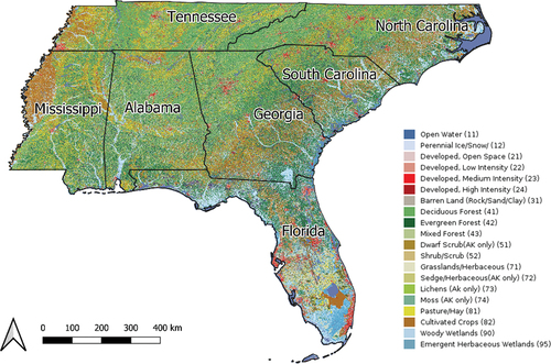
Figure 1. Study area located in the US southeastern states, including North Carolina, South Carolina, Alabama, Florida, Georgia, Mississippi, Tennessee. The base map is NLCD1992, which shows that the study area has extensive forest coverage.

2. Study area and data collection

2.1. Study site

Located in the southeastern of the United States, the seven states of the study area cover a total area of 916,993 km² that include both lowlands and highlands. While the region is dominated by rolling hills, plateaus and rich river valleys in the north, the south is characterized by beaches, swamps, and wetlands. The region has a subtropical monsoon climate in the south transitioning to a temperate climate to the north. The summer is long, hot, and humid, while the winter is short and warm. The average annual precipitation in this area ranges from about 109 to 107 cm. The forest coverage of the seven states is between 50.68% and 70.57% respectively, of which Alabama, South Carolina, Georgia, and Mississippi have the largest forest coverage, all above 65%. Southern forests have the highest planted timberland rates in the US (71% of all planted timberland), of which Alabama has 33% planted timberland rate, 32% for Georgia, 32% for Mississippi, 31% for Florida, and 31% for Louisiana, all have the highest proportions of planted to total timberland, nationally (Oswalt et al. 2019). In the southern planted timberland, the main forest types are Loblolly pine (Pinus taeda) and shortleaf pine (Pinus echinate), which account for 71% of all planted forests in the South (Figure 1).

2.2. Data collection

2.2.1. TPO survey data

The TPO survey data (USDA Forest Service 2019) were acquired from Forest Inventory and Analysis (FIA) national program of the United States Forest Service (USFS). FIA carried out state-level TPO studies to investigate round wood uses for industrial and non-industrial purposes in a given state using ground-based survey methods. In order to determine the geographic origin, harvest date, volume, species, and use of harvested roundwood products, FIA canvasses all primary wood-using mills, harvest sites, residential users, and commercial producers that harvest and sell wood products for selected study years (Johnson 2001; Woodbury, Smith, and Heath 2007). For each study year, the collected data are compiled to produce a TPO report that provides county level wood product estimates for that year. The survey data include county-level estimation of industrial roundwood (sawlog and pulpwood), fuelwood, chips, post, poles, and so on. The industrial roundwood estimation mainly consists of the estimates of industrial hardwood and industrial softwood. In this study, only industrial roundwood and fuelwood were considered, as they are the main components of total roundwood production in the study region. These included softwood saw log (SS), softwood pulpwood (SP), softwood fuelwood (SF), hardwood saw log (HS), hardwood pulpwood (HP), and hardwood fuelwood (HF).

Table 1 lists the TPO reports available from 1995 to 2009 over the study region. All of the 7 states had data for 1995, 1999, 2005, 2007, and 2009. Except for Mississippi, the other 6 states also had data for 1997 and 2003. In addition, TPO reports were available for Georgia, North Carolina, South Carolina, and Tennessee in 2001. While Mississippi had TPO data for only 5 years, it is the only state that had data for 2002. As the only data source that can provide survey-based TPO estimates for individual counties during a specific year, the TPO reports are highly valuable for calibrating and validating models designed to produce county-level TPO estimates on an annual basis (C. Huang, Ling, and Zhu 2015).

Table 1. Years in which county-level TPO survey data are available for each state, “x” indicates the data is available for that year in that state.

State	1995	1997	1999	2001	2002	2003	2005	2007	2009
Alabama (AL)	x	x	x			x	x	x	x
Florida (FL)	x	x	x			x	x	x	x
Georgia (GA)	x	x	x	x		x	x	x	x
Mississippi (MS)	x		x		x		x	x	x
North Carolina (NC)	x	x	x	x		x	x	x	x
South Carolina (SC)	x	x	x	x		x	x	x	x
Tennessee (TN)	x	x	x	x		x	x	x	x

Source: USDA Forest Service: https://www.fia.fs.usda.gov/program-features/tpo/.

The average annual timber production volumes for hardwood, softwood, and both calculated from the available TPO reports in the 7 states are listed in Table 2.

Table 2. Average annual timber production volume (in thousand cubic meters) in each state based on the survey data listed in Table 1.

State	Hardwood	Softwood	Total
Alabama	9733.46	23,986.03	33,719.49
Florida	1574.83	13,006.01	14,580.83
Georgia	7831.17	27,986.87	35,818.03
Mississippi	7675.47	19,330.68	27,006.15
North Carolina	9217.77	14,760.85	23,978.62
South Carolina	4299.35	13,804.73	18,104.08
Tennessee	7409.33	2328.98	9738.31

2.2.2. Forest disturbance and land cover data

Forest disturbance data used in this study included 30 m disturbance maps derived using Landsat time series stacks (LTSS) and the Vegetation Change Tracker (VCT) algorithm (Huang et al. 2011; Zhao et al. 2018). An LTSS is a stack of Landsat images assembled for a World Reference System (WRS) path/row tile to provide clear view observations at a regular time step (Huang, Goward, Masek, et al. 2009). An annual LTSS consists of an individual Landsat acquisition or a composited image for each year to provide cloud-free or near cloud-free (<5% cloud cover) time series observations for the summer leaf-on season of a multi-year study period.

VCT is an automated algorithm designed to analyze an LTSS to produce disturbance products (Huang et al. 2010). This is achieved through two major steps. First, each image in the LTSS is analyzed to mask water, cloud, and cloud shadow pixels and to select forest samples from densely forested areas. Based on these forest samples, an Integrated Forest Z-score (IFZ) index is calculated for each pixel using the following formula:

(1) $\mathit{IFZ}=\sqrt{\frac{1}{3}\sum _{\mathit{band}3,5,7}\left(\frac{b_i-{\bar{b}}_{\mathit{i}}}{\mathit{S}{D}_i}\right)}$(1)

where $b_i$ denotes the pixel’s value in band i; and ${\bar{b}}_{\mathit{i}}$ and $\mathit{S}{D}_i$ standard deviation of the forest samples selected above. IFZ index is a non-negative and inverse indicator of the likelihood of a pixel being a forest pixel. The higher IFZ value, the more likely the pixel being a non-forest pixel. On the contrary, the closer IFZ is to zero, the more likely the pixel is to be a forest pixel. Next, the IFZ time series of each pixel is analyzed to determine whether that pixel had forest cover during at least part of the study period. If yes, the pixel is further evaluated to determine whether disturbances occurred during the study period. If yes, the disturbance year is determined for each detected disturbance event and its disturbance magnitude is calculated as the change in IFZ.

The VCT algorithm has been used to produce 30 m disturbance products for the conterminous U.S. from 1986 to 2010 (Zhao et al. 2018). The disturbance products used in this study was generated as part of that effort, which were extended to 2015.

Because the TPO data are divided into softwood and hardwood products, a land cover map from the National Land Cover Database (NLCD) was used in this study to provide information on the distribution of deciduous (hardwood) and evergreen (softwood) forests over the study region. NLCD is an ongoing US-wide land cover mapping effort that has resulted in NLCD products for many epochs since 1990s. The 1992 map should provide a better characterization of pre-disturbance forest distributions than later NLCD products, and hence was used in this study.

3. Methods

3.1. Preparation of predictor variables

A key hypothesis in modeling TPO from disturbance data is that timber harvest volume should be correlated with Landsat-based disturbance estimates (Huang, Ling, and Zhu 2015; Ling, Baiocchi, and Huang 2016). Given the disturbance products, theoretically, Harvested Timber Volume (HTV) could be calculated as the product of stock density, harvest area and harvest intensity, and TPO would be the difference between HTV and slash (the debris of trees left in the field after harvesting). However, although logging is a dominant disturbance agent in the southeast, it is not the only. As a result, the disturbance data can only provide proxy information for logging. Therefore, direct calculation of TPO using Landsat-based disturbance estimates and available ancillary data was not possible. Instead, regression models such as OLS and RF were used to establish relationships between TPO survey data and disturbance data.

Since the TPO survey data were only available at the county level, the 30 m disturbance data were aggregated to produce county-level estimates. Based on lessons learned from C. Huang et al. (2015), the disturbance areas within each county in any given year of the study period were calculated at four IFZ disturbance magnitude (IFZ-DM, Table 3), since disturbance intensity is directly related to the amount of wood harvested. Further, these areas were calculated for disturbances over deciduous/hardwood, evergreen/softwood, and mixed forest pixels as mapped by the 1992 NLCD land cover map to differentiate the wood products in different wood types. Therefore, a total of 12 disturbance area values were calculated for each county in each disturbance year.

Table 3. IFZ disturbance magnitude (IFZ-DM) levels at which county level disturbance areas were calculated.

Disturbance magnitude Level	Threshold values
1	IFZ-DM ≤ 3
2	3 < IFZ-DM ≤ 6
3	6 < IFZ-DM ≤ 9
4	IFZ-DM ≥ 9

Another issue that needed to be addressed was that the effective date range of the TPO survey data for any given year does not match that of the disturbances mapped by the VCT for that year. The survey data is collected from the beginning to the end of a year (hereby called survey year), while most disturbance events mapped for a year by the VCT algorithm could occur any time between the acquisition dates of the images used for that year and the previous year. Further, due to residual clouds and other data quality issues, the actual disturbance year could also be one year before or after the mapped disturbance year (Huang et al. 2010; Thomas et al. 2011). To reduce the influence of such temporal mismatches, for each TPO modeling/prediction year it was necessary to consider two more years – one immediately before and one immediately after that year (Huang, Ling, and Zhu 2015; Ling, Baiocchi, and Huang 2016). Therefore, a total of 36 predictor variables (12 per year x 3 years) were used to model and predict TPO for any given year.

3.2. Modeling approaches

Two modeling algorithms were examined in this study, including the Ordinary Least Square linear regression and the Random Forest algorithm. The OLS linear regression model can be written as:

(2) $Y_{\mathit{it}}=\mathit{\alpha }+\mathit{\beta }{X}_{\mathit{it}}+{\epsilon }_{\mathit{it}}$(2)

where $Y_{\mathit{it}}$, $X_{\mathit{it}}$, and ${\epsilon }_{\mathit{it}}$ are the TPO value for a specific wood product type, a vector of the 36 predictor variables as described in Section 3.1, and model residual for county i in year t, and α and β are the regression intercept and the slope vector for the predictor variables, respectively. Both α and β are independent of the county index i and year index t.

Random Forest is an ensemble learning method based on classification and regression trees (Breiman 2001). The algorithm ensembles a large number of trees where each tree is developed using a random subset of the predictor variables and is trained using a random subset of the training data (Breiman 1996). With demonstrated robustness for addressing both classification and regression problems (Du et al. 2015; Pal 2005; Rodriguez-Galiano et al. 2012), it has been used in many forest remote sensing applications (Liu et al. 2019; Pearse et al. 2017; Ploton et al. 2017).

The two approaches were used to model the volume of each of the 6 individual product types, namely, softwood saw log (SS), softwood pulpwood (SP), softwood fuelwood (SF), hardwood saw log (HS), hardwood pulpwood (HP), and hardwood fuelwood (HF). The total volume of the 6 types, referred to as total TPO throughout this study, was also modeled. The robustness of OLS and RF models was evaluated through a ten-fold cross-validation method based on 4592 samples. In this method, the reference samples were divided evenly into 10 random subsets. Each subset was used to evaluate a model calibrated using the remaining 9 subsets. This was repeated 10 times such that each time a different subset was used as test data. Results from all 10 experiments were combined to produce representative accuracy estimates for the final model to be derived using all reference samples.

4. Results

4.1. Comparative performances of OLS and RF for TPO modeling

Several wood product types were modeled reasonably well using both OLS and RF. Comparison of the predicted values against the survey data resulted in coefficient of determination (R²) values of 0.5 or higher for multiple wood product types in several states (Tables 4 and 5). Except for Tennessee, both OLS and RF resulted in better R² values on the other 6 states for the softwood types than for the hardwood types, indicating that relationships between timber output for hardwood types and the disturbance data were not as good as those for softwood types. Among the 7 states, South Carolina’s TPO appeared to be more difficult to model. Except for the hardwood sawlog (HS) in Florida, the R² values derived for this state were lower than those for the other 6 states for all 6 wood types.

Table 4. R² values of the relationships between TPO values predicted by OLS and survey data derived through 10-fold cross-validation.

Product type	State
	AL	FL	GA	MS	TN	NC	SC	All 7 States
SP	0.61	0.41	0.56	0.36	0.54	0.54	0.27	0.58
SS	0.62	0.48	0.40	0.50	0.08	0.57	0.26	0.52
SF	0.63	0.65	0.52	0.54	0.33	0.61	0.35	0.31
HP	0.45	0.06	0.12	0.24	0.51	0.10	0.00*	0.33
HS	0.21	0.00*	0.14	0.15	0.29	0.34	0.05	0.29
HF	0.56	0.13	0.19	0.56	0.24	0.15	0.01	0.19

Except those indicated by the “*”, all R² values were statistically different from 0 with a p-value < 0.05. Abbreviations for product type: SS – softwood saw log, SP – softwood pulpwood, SF – softwood fuelwood, HS – hardwood saw log, HP – hardwood pulpwood, and HF – hardwood fuelwood. See Table 1 for the abbreviations for the 7 states.

Table 5. R² values of the relationships between TPO values predicted by RF and survey data derived through 10-fold cross-validation.

Product type	State
	AL	FL	GA	MS	TN	NC	SC	All 7 States
SP	0.63	0.57	0.64	0.60	0.62	0.56	0.37	0.62
SS	0.63	0.66	0.48	0.66	0.18	0.60	0.41	0.59
SF	0.59	0.71	0.56	0.57	0.44	0.62	0.43	0.37
HP	0.55	0.23	0.23	0.28	0.54	0.18	0.04	0.41
HS	0.34	0.05	0.20	0.21	0.46	0.41	0.18	0.35
HF	0.55	0.24	0.29	0.44	0.34	0.30	0.10	0.29

All R² values were statistically different from 0 with a p-value < 0.05. See Table 3 for abbreviations for the states and product types.

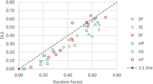
Overall, RF performed better in modeling TPO volume than the OLS. Its R² values were higher than those derived using OLS for most of the states and wood types (Figure 2). While the differences were small in some cases, on average, the use of RF instead of the OLS resulted in an improvement of 0.08 in the R² value, and the improvements exceeded 0.1 for at least one of the 6 wood types in each of the 7 states. OLS had substantially better performance than RF for only two cases: softwood fuelwood (SF) in Alabama and hardwood fuelwood (HF) in Mississippi, suggesting that in these two cases the RF models might have overfitting issues.

Figure 2. Coefficient of determination (R²) values derived by comparing survey data and values predicted by OLS (y-axis) and Random Forest (x-axis) through 10-fold cross validation. Each point represents one wood product type in one state. The two right most points were from Georgia. Abbreviations for product type: SS – softwood saw log, SP – softwood pulpwood, SF – softwood fuelwood, HS – hardwood saw log, HP – hardwood pulpwood, and HF – hardwood fuelwood.

4.2. Spatial-temporal variability of TPO in the southeast

Given the overall better performance of Random Forest as compared to Ordinary Least Square for TPO modeling, it was used to produce annual TPO volume estimates for all 7 states in the southeast. From 1986 to 2015, the region produced more than 5 × 10⁹ m³ harvested wood products, including 3.7 × 10⁹ m³ softwood products and 1.6 × 10⁹ m³ hardwood products (Table 6). Of the 7 states, Georgia and Alabama had the highest TPO values, while Tennessee produced the least amount of wood products, although the state was larger and had more forest land than South Carolina. Tennessee was also the only state that produced more hardwood products than softwood products. All other 6 states had higher total TPO volumes for the softwood types than for the hardwood types.

Table 6. Estimated 30-year (1986–2015) total TPO volume (10³ m³) for the 7 states in the southeast United States.

State	Product type
	SP	SS	SF	HP	HS	HF	All Types
AL	330,487	404,207	7269	175,158	87,575	43,301	1,065,097
FL	235,876	215,251	4439	45939	16,294	18,238	559,074
GA	439,448	496,884	11,946	148,388	104,004	62,604	1,309,772
MS	238,282	362,725	6186	146,179	76,195	35,335	878,470
TN	45,456	58,719	3152	72,831	105,075	36,378	324,335
NC	159,241	239,199	6613	111,021	94,753	50,262	675,047
SC	206,721	215,908	4521	61,986	36,193	24,301	567,153
All States	1,655,511	1,992,892	44,126	761,500	520,089	270,420	5,378,947

See Table 3 for abbreviations for the states and product types.

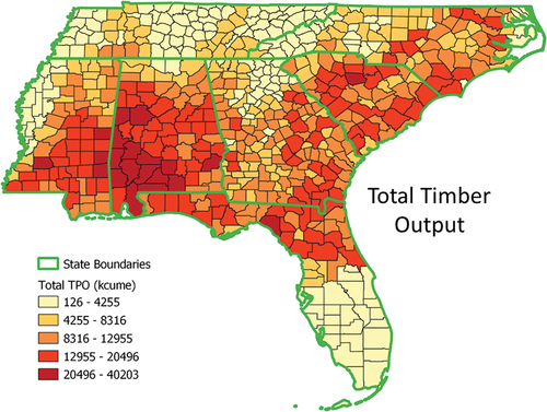
The derived TPO estimates had large variations among the counties within each state. Counties that had high TPO volumes were mostly in Alabama, South Carolina, the central and southern part of Mississippi, northern Florida, and the east part of North Carolina (Figure 3). Most counties in Tennessee, southern Florida, western Mississippi, north central Georgia, and the northern most part of Alabama had low TPO volumes.

Figure 3. County-level total TPO values predicted by the Random Forest model for the 30-year study period (1986–2015).

Overall, the average state-level annual TPO volume estimates calculated from the 30-year record were comparable to those derived from the TPO survey data, with the 30-year averages being higher than the survey data for the softwood types in some states (Figure 4). In particular, the 30-year average TPO values for softwood sawlog (SS) and softwood pulpwood (SP) in Mississippi were 14.6 and 16.6 × 10⁶ m³/year, whereas the averages from the survey data were 12.7 and 12.9 × 10⁶ m³/year, respectively. Alabama’s 12.5 × 10⁶ m³/year 30-year average value for softwood sawlog was ~2 × 10⁶ m³/year higher than the 11.6 × 10⁶ m³/year average value calculated from survey data. A detailed examination of the annual TPO estimates over the 30-year study period revealed that the TPO volumes had large variations over time (Figure 5). The highest TPO volumes in Georgia were found before 1990 and after 2010, but those years were not represented by the TPO survey data. This may explain why the 30-year averages were substantially higher than the averages from the survey data. The slightly higher 30-year average values than averages from the survey data in Alabama, Florida, Mississippi, and South Carolina were likely due to similar reasons.ed using discontinuous TPO survey data and annual remote sensing data.

Figure 4. Comparison of the average annual TPO volume calculated from the 30-year record derived through this study and available TPO survey data. Each point represents one wood product type in one state. The two right most points were from Georgia. Abbreviations for product type: SS – softwood saw log, SP – softwood pulpwood, SF – softwood fuelwood, HS – hardwood saw log, HP – hardwood pulpwood, and HF – hardwood fuelwood.

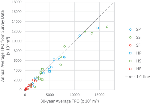
Figure 5. Annual TPO volume predicted using the RF algorithm for the seven states in the southeast U.S. Total TPO refers to the total volume of the 6 product types considered in this study.

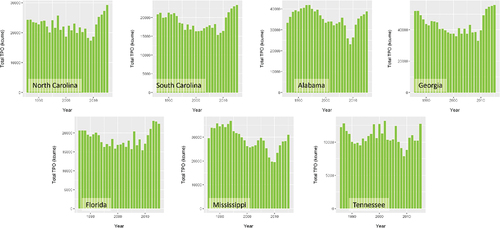
The temporal dynamics of the TPO record over the 30-year study period had similarities and differences among the 7 states (Figure 5). The 2007–2008 economic downturn appeared to have large impact on wood product output across the region. All 7 states had the lowest TPO volumes around that time, which were followed by sharp increases in the next few years. Several states also had high TPO volumes before or around early 1990s that were followed relatively lower TPO values throughout much of the 1990s and 2000s, including Florida, Georgia, and South Carolina, whereas Tennessee’s TPO estimates were relatively high during that period. Both Alabama and Mississippi had high TPO volumes over multiple years that peaked in early to mid-1990s, which were followed by a smaller peak centered around 2005.

5. Discussion and conclusions

This paper explored two approaches for deriving annual TPO estimates, including the Ordinary Least Square linear regression and the Random Forest regression tree algorithm. RF appeared to be more robust than OLS for modeling TPO volumes. Cross-validation results revealed that on average, the coefficient of determination (R²) between predicted and survey data was improved by 0.08 when TPO was modeled using RF instead of the OLS.

Predictions by the RF algorithm revealed that from 1986 to 2015, the 7 states in the Southeast produced more than 5 × 10⁹ m³ wood products, of which over 40% were contributed by Georgia and Alabama. The average annual TPO estimates calculated from the 30-year record were comparable to those derived from the TPO survey data, with the 30-year averages being higher than the survey data in some states. This was mainly due to large temporal variations of the TPO estimates over the 30-year study period, with many of the years in the first and/or last 5–10 years of the study period having high TPO values that were not represented by the survey data.

The annual TPO record derived through this study complements available TPO survey data in several ways. First, the time span of the derived data record (1986–2015) is twice as long as that covered by the TPO survey data used in this study (1995–2009). Second, the annual time step of the derived data can provide more temporal details than the survey data, which typically skipped one or more years for each of the 7 states in the southeast (Table 1). Third, the years during which survey data are available in one state are not always the same as those in other states, making it difficult to calculate survey-based TPO volumes for regions consisting of multiple states. As an annual dataset derived consistently across the entire region and over time, the TPO record derived through this study makes it possible to assemble a complete TPO dataset that covers all 7 states for any year between 1986 and 2015. Of course, while the TPO survey data were not spatially or temporally as comprehensive as the annual TPO record derived through this study, the survey data were critically important for calibrating the RF models. There are no other data sources that can provide reliable and comprehensive information on harvested timber volume like the TPO survey data.

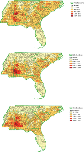
Modeled based on forest disturbances mapped using satellite imagery, the TPO data derived through this study can provide an observational basis for calculating the amount of C transferred from the standing biomass to the wood product through logging and for partitioning of harvested C among different wood product pools. Most carbon models assume that carbon can be stored in sawlogs for hundreds of years, while pulp wood can only store carbon for a decade or so. The carbon consequences of fuel woods are more complicated. While the carbon in fuelwoods is released almost immediately following harvest (Gong et al. 2022; Houghton and Nassikas 2017), they provide substitution benefits by offsetting some fossil fuel uses. Figure 6 shows that not only the harvested timber volumes but also their partitioning among the three product types can differ substantially among different counties. Considering the annual temporal details available for each product type for each county, the TPO record derived through this study may allow more reliable and more detailed estimation of C fluxed related to wood products in future research.

Figure 6. 25-year total production volumes of fuel wood, pulp wood, and sawlog. The volumes of each wood product vary greatly among the counties.

With demonstrated robustness over 7 states in the Southeast, the RF-based modeling framework developed in this study might be applicable in other regions of the United States. Annual forest disturbances have already been mapped for the conterminous U.S. (CONUS) using time series Landsat observations from 1986 to 2010 (Zhao et al. 2018). There are also other efforts dedicated to producing comprehensive disturbance products for CONUS (Brown et al. 2020). As of the Huang, Ling, and Zhu (2015) study, every state in CONUS had TPO survey data for at least two years. Therefore, it is possible to expand the geographic domain of this study to the entire CONUS. Although approaches have been proposed for producing TPO survey data on an annual basis [3], this RF-based modeling framework could complement the TPO program in that it can be used to fill gaps in the existing survey data, which cannot be filled using the existing or proposed TPO survey methods. Further, this modeling framework might also be applicable in other regions or countries where TPO-like survey data have been collected.

It should be noted that several data products that became available recently might be better than the data used in this study and hence could be used to improve TPO modeling. One is a disturbance intensity dataset developed by Tao et al. (2019), which quantifies the percentage of the basal area removed by disturbance events mapped by VCT. Calibrated using basal area removal data calculated from field observations, this dataset should provide a more reliable measure of logging intensity that in turn should result in better estimation of the timber output from logging. Another dataset is the disturbance attribution data developed by Schleeweis et al. (2020), which explicitly mapped forest harvest and several other disturbance agents across CONUS. Excluding disturbances that are unlikely to result in timber output likely will improve TPO estimation. Another desirable dataset is annual aboveground biomass. Such a dataset could be used to calculate pre-harvest C stock, which is needed together with a measure of disturbance intensity to calculate harvested C.

Acknowledgements

This study was made possible by NASA’s Carbon Cycle Science and Land Cover and Land Use Change Programs (Grant No. NNX14AM39G, NNX14AD89G, and NNX15AE79G), the Laboratory of Environmental Model and Data Optima (EMDO, Grant No. 2106313), and Pie-Australia (Grant No. 19102901). The TPO survey data were downloaded from the SRS FIA Data Center (https://www.fs.usda.gov/srsfia/data_center/index.shtml). Additional support was provided by the Department of Geographical Sciences of the University of Maryland. We thank Dr. Jack (Jianguo) Ma for his long-term support.

Disclosure statement

No potential conflict of interest was reported by the author(s).

Data availability statement

The data that support the findings of this study are available from the corresponding author, W.G., upon reasonable request.

Additional information

Funding

This work was supported by the National Aeronautics and Space Administration [grant number NNX14AD89G]; Pie-Australia [grant number 19102901]; the Laboratory of Environmental Model and Data Optima [grant number 2106313].

Notes on contributors

Weishu Gong

Weishu Gong received her PhD from the Department of Geographical Sciences, University of Maryland, College Park. Currently, she works there as a Post-Doctoral Associate. Her research interests include forest carbon dynamics and land use/land cover change. Her ongoing projects mostly involve estimating carbon fluxes from forest disturbances by combining forest inventory data with grid-based remote sensing datasets.

Chengquan Huang

Chengquan Huang is a research professor at the Department of Geographical Sciences, University of Maryland, College Park. He has devoted a decade to studies of land cover and vegetation dynamics using remotely sensed data. He has been engaged in several projects that were national to continental in scale, including the USGS Multi-Resolution Land Characteristics (MRLC) 2001 project, the joint USGS-US Forest Service LANDFIRE project, the NASA LEDAPS project, and the NASA North American Forest Dynamics project. He is currently leading efforts to quantify forest change at national to global scales using Landsat data, and is developing approaches for mapping forest structure and biomass change by integrating field inventory data, airborne or space-borne lidar, and Landsat derived forest disturbance history.

Feng Zhao

Feng Zhao graduated from Boston University and is presently a remote sensing scientist with a research specialization in terrestrial ecosystem mapping. His research focused on developing novel data inputs, improved algorithms, and thematic maps for regional and continental scale land cover dynamics, biomass and carbon stocks. Those maps are critical to natural resource management and climate change studies. His current research includes asset level dynamics monitoring, which will be used to evaluate the reliance of assets on physical environment as well as the resilience of assets to the changing physical environment.

Jiaming Lu

Jiaming Lu is a PhD candidate from the Department of Geographical Sciences, University of Maryland. She is interested in studying forest disturbance dynamics, and mapping key forest attributes (e.g. forest age structure) using remote sensing and forest inventory data.

References

- Birdsey, R. 2004. “Data Gaps for Monitoring Forest Carbon in the United States: An Inventory Perspective.” Environmental Management 33 (S1). https://doi.org/10.1007/s00267-003-9113-6.
- Breiman, L. 1996. “Bagging Predictors.” Machine Learning 24 (2): 123–140. https://doi.org/10.1007/BF00058655.
- Breiman, L. 2001. “Random Forests.” Machine Learning 45 (August): 5–32. https://doi.org/10.1023/A:1010933404324.
- Brown, J. F., H. J. Tollerud, C. P. Barber, Q. Zhou, J. L. Dwyer, J. E. Vogelmann, T. R. Loveland, et al. 2020. “Lessons Learned Implementing an Operational Continuous United States National Land Change Monitoring Capability: The Land Change Monitoring, Assessment, and Projection (LCMAP) Approach.” Remote Sensing of Environment 238 (March): 111356. https://doi.org/10.1016/J.RSE.2019.111356.
- Chander, G., B. L. Markham, and D. L. Helder. 2009. “Summary of Current Radiometric Calibration Coefficients for Landsat MSS, TM, ETM+, and EO-1 ALI Sensors.” Remote Sensing of Environment 113 (5): 893–903. https://doi.org/10.1016/j.rse.2009.01.007.
- Coulston, J. W., J. A. Westfall, D. N. Wear, C. B. Edgar, S. P. Prisley, T. B. Treiman, R. C. Abt, and W. B. Smith. 2018. “Annual Monitoring of US Timber Production: Rationale and Design.” Forest Science 64 (5): 533–543. https://doi.org/10.1093/forsci/fxy010.
- Du, P., A. Samat, B. Waske, S. Liu, and Z. Li. 2015. “Random Forest and Rotation Forest for Fully Polarized SAR Image Classification Using Polarimetric and Spatial Features.” ISPRS Journal of Photogrammetry and Remote Sensing 105 (July): 38–53. https://doi.org/10.1016/j.isprsjprs.2015.03.002.
- Gong, W., C. Huang, R. A. Houghton, A. Nassikas, F. Zhao, X. Tao, J. Lu, and K. Schleeweis. 2022. “Carbon Fluxes from Contemporary Forest Disturbances in North Carolina Evaluated Using a Grid-Based Carbon Accounting Model and Fine Resolution Remote Sensing Products.” Science of Remote Sensing 5 (January): 100042. https://doi.org/10.1016/j.srs.2022.100042.
- Hansen, M. C., P. V. Potapov, R. Moore, M. Hancher, S. A. Turubanova, A. Tyukavina, D. Thau, et al. 2013. “High-Resolution Global Maps of 21st-Century Forest Cover Change.” Science 342 (6160): 850–853. https://doi.org/10.1126/science.1244693.
- Harris, N. L., S. C. Hagen, S. S. Saatchi, T. R. H. Pearson, C. W. Woodall, G. M. Domke, B. H. Braswell, et al. 2016. “Attribution of Net Carbon Change by Disturbance Type Across Forest Lands of the Conterminous United States.” Carbon Balance and Management 11 (1): 24. https://doi.org/10.1186/s13021-016-0066-5.
- Harris, N. L., S. C. Hagen, S. S. Saatchi, T. R. H. H. Pearson, C. W. Woodall, G. M. Domke, B. H. Braswell, et al. 2016. “Attribution of Net Carbon Change by Disturbance Type Across Forest Lands of the Conterminous United States.” Carbon Balance and Management 11 (1): 24. https://doi.org/10.1186/s13021-016-0066-5.
- Ho, T. K. 1998. “The Random Subspace Method for Constructing Decision Forests.” IEEE Transactions on Pattern Analysis and Machine Intelligence 20 (8): 832–844. https://doi.org/10.1109/34.709601.
- Houghton, R. A., and A. Nassikas. 2017. “Global and Regional Fluxes of Carbon from Land Use and Land Cover Change 1850–2015.” Global Biogeochemical Cycles 31 (3): 456–472. https://doi.org/10.1002/2016GB005546.
- Huang, C., S. N. Goward, J. G. Masek, F. Gao, E. F. Vermote, N. Thomas, K. Schleeweis, et al. 2009. “Development of Time Series Stacks of Landsat Images for Reconstructing Forest Disturbance History.” International Journal of Digital Earth 2 (3): 195–218. https://doi.org/10.1080/17538940902801614.
- Huang, C., S. N. Goward, J. G. Masek, N. Thomas, Z. Zhu, and J. E. Vogelmann. 2010. “An Automated Approach for Reconstructing Recent Forest Disturbance History Using Dense Landsat Time Series Stacks.” Remote Sensing of Environment 114 (1): 183–198. https://doi.org/10.1016/j.rse.2009.08.017.
- Huang, C., S. N. Goward, K. Schleeweis, N. Thomas, J. G. Masek, and Z. Zhu. 2009. “Dynamics of National Forests Assessed Using the Landsat Record: Case Studies in Eastern United States.” Remote Sensing of Environment 113 (7): 1430–1442. https://doi.org/10.1016/j.rse.2008.06.016.
- Huang, C., P. Y. Ling, and Z. Zhu. 2015. “North Carolina’s Forest Disturbance and Timber Production Assessed Using Time Series Landsat Observations.” International Journal of Digital Earth 8 (12): 947–969. https://doi.org/10.1080/17538947.2015.1034200.
- Huang, C., K. Schleeweis, N. Thomas, and S. Goward. 2011. “Forest Dynamics within and Around Olympic National Park Assessed Using Time-Series Landsat Observations.” In Remote Sensing of Protected Lands, 75–94. TA - TT -. CRC Press. https://doi.org/10.1201/b11453-6.
- Huang, X., and J. R. Jensen. 1997. “A Machine-Learning Approach to Automated Knowledge-Base Building for Remote Sensing Image Analysis with GIS Data.” Photogrammetric Engineering & Remote Sensing 63 (10): 1185–1194.
- Johnson, T. G. 2001. United States Timber Industry - An Assessment of Timber Product Output and Use, 1996. Asheville, NC: U.S. Department of Agriculture, Forest Service, Southern Research Station.
- Kennedy, R. E., Z. Yang, J. Braaten, C. Copass, N. Antonova, C. Jordan, and P. Nelson. 2015. “Attribution of Disturbance Change Agent from Landsat Time-Series in Support of Habitat Monitoring in the Puget Sound Region, USA.” Remote Sensing of Environment 166 (September): 271–285. https://doi.org/10.1016/j.rse.2015.05.005.
- Kennedy, R. E., Z. Yang, W. B. Cohen, E. Pfaff, J. Braaten, and P. Nelson. 2012. “Spatial and Temporal Patterns of Forest Disturbance and Regrowth within the Area of the Northwest Forest Plan.” Remote Sensing of Environment 122 (July): 117–133. https://doi.org/10.1016/j.rse.2011.09.024.
- Ling, P. Y., G. Baiocchi, and C. Huang. 2016. “Estimating Annual Influx of Carbon to Harvested Wood Products Linked to Forest Management Activities Using Remote Sensing.” Climatic Change 134 (1–2): 45–58. https://doi.org/10.1007/s10584-015-1510-3.
- Lippke, B., E. Oneil, R. Harrison, K. Skog, L. Gustavsson, and R. Sathre. 2011. “Life Cycle Impacts of Forest Management and Wood Utilization on Carbon Mitigation: Knowns and Unknowns.” Carbon Management 2 (3): 303–333. https://doi.org/10.4155/cmt.11.24.
- Liu, Y., W. Gong, Y. Xing, X. Hu, and J. Gong. 2019. “Estimation of the Forest Stand Mean Height and Aboveground Biomass in Northeast China Using SAR Sentinel-1B, Multispectral Sentinel-2A, and DEM Imagery.” Isprs Journal of Photogrammetry & Remote Sensing 151 (November 2018): 277–289. https://doi.org/10.1016/j.isprsjprs.2019.03.016.
- Mäkelä, H., and A. Pekkarinen. 2001. “Estimation of Timber Volume at the Sample Plot Level by Means of Image Segmentation and Landsat TM Imagery.” Remote Sensing of Environment 77 (1): 66–75. https://doi.org/10.1016/S0034-4257(01)00194-8.
- Mishra, N., D. Helder, J. Barsi, and B. Markham. 2016. “Continuous Calibration Improvement in Solar Reflective Bands: Landsat 5 Through Landsat 8.” Remote Sensing of Environment 185 (November): 7–15. https://doi.org/10.1016/j.rse.2016.07.032.
- Oswalt, S. N., W. B. Smith, P. D. Miles, and S. A. Pugh. 2019. Forest Resources of the United States, 2017. Washington, D.C: U.S. Department of Agriculture, Forest Service. https://doi.org/10.2737/WO-GTR-97.
- Pal, M. 2005. “Random Forest Classifier for Remote Sensing Classification.” International Journal of Remote Sensing 26 (1): 217–222. https://doi.org/10.1080/01431160412331269698.
- Pearse, G. D., J. Morgenroth, M. S. Watt, and J. P. Dash. 2017. “Optimising Prediction of Forest Leaf Area Index from Discrete Airborne Lidar.” Remote Sensing of Environment 200 (July): 220–239. https://doi.org/10.1016/j.rse.2017.08.002.
- Ploton, P., N. Barbier, P. Couteron, C. M. M. Antin, N. Ayyappan, N. Balachandran, N. Barathan, et al. 2017. “Toward a General Tropical Forest Biomass Prediction Model from Very High Resolution Optical Satellite Images.” Remote Sensing of Environment 200 (July): 140–153. https://doi.org/10.1016/j.rse.2017.08.001.
- Rodriguez-Galiano, V. F., B. Ghimire, J. Rogan, M. Chica-Olmo, and J. P. Rigol-Sanchez. 2012. “An Assessment of the Effectiveness of a Random Forest Classifier for Land-Cover Classification.” ISPRS Journal of Photogrammetry and Remote Sensing 67 (1): 93–104. https://doi.org/10.1016/j.isprsjprs.2011.11.002.
- Ruddell, S., R. Sampson, M. Smith, R. Giffen, J. Cathcart, J. Hagan, D. Sosland, et al. 2007. “The Role for Sustainably Managed Forests in Climate Change Mitigation.” Journal of Forestry 105 (6): 314–319.
- Schleeweis, K. G., G. G. Moisen, T. A. Schroeder, C. Toney, E. A. Freeman, S. N. Goward, C. Huang, and J. L. Dungan. 2020. “US National Maps Attributing Forest Change: 1986–2010.” Forests 11 (6): 1–20. https://doi.org/10.3390/F11060653.
- Shao, Y., and R. S. Lunetta. 2012. “Comparison of Support Vector Machine, Neural Network, and CART Algorithms for the Land-Cover Classification Using Limited Training Data Points.” ISPRS Journal of Photogrammetry and Remote Sensing 70 (June): 78–87. https://doi.org/10.1016/j.isprsjprs.2012.04.001.
- Tao, X., C. Huang, F. Zhao, K. Schleeweis, J. Masek, and S. Liang. 2019. “Mapping Forest Disturbance Intensity in North and South Carolina Using Annual Landsat Observations and Field Inventory Data.” Remote Sensing of Environment 221 (May 2018): 351–362. https://doi.org/10.1016/j.rse.2018.11.029.
- Thomas, N. E., C. Huang, S. N. Goward, S. Powell, K. Rishmawi, K. Schleeweis, and A. Hinds. 2011. “Validation of North American Forest Disturbance Dynamics Derived from Landsat Time Series Stacks.” Remote Sensing of Environment 115 (1): 19–32. https://doi.org/10.1016/j.rse.2010.07.009.
- Trotter, C. M., J. R. Dymond, and C. J. Goulding. 1997. “Estimation of Timber Volume in a Coniferous Plantation Forest Using Landsat TM.” International Journal of Remote Sensing 18 (10): 2209–2223. https://doi.org/10.1080/014311697217846.
- USDA Forest Service. 2019. “Timber Products Output.” https://www.nrs.fs.fed.us/fia/topics/tpo/.
- Verrelst, J., J. Munoz, L. Alonso, J. Delegido, J. P. Rivera, G. Camps-Valls, J. Moreno, et al. 2012. “Machine Learning Regression Algorithms for Biophysical Parameter Retrieval: Opportunities for Sentinel-2 and -3.” Remote Sensing of Environment 118:127–139. https://doi.org/10.1016/j.rse.2011.11.002.
- White, J. C., M. A. Wulder, T. Hermosilla, N. C. Coops, and G. W. Hobart. 2017. “A Nationwide Annual Characterization of 25 Years of Forest Disturbance and Recovery for Canada Using Landsat Time Series.” Remote Sensing of Environment 194 (June): 303–321. https://doi.org/10.1016/j.rse.2017.03.035.
- Woodbury, P. B., J. E. Smith, and L. S. Heath. 2007. “Carbon Sequestration in the U.S. Forest Sector from 1990 to 2010.” Forest Ecology and Management 241 (1–3): 14–27. https://doi.org/10.1016/j.foreco.2006.12.008.
- Zeng, N. 2008. “Carbon Sequestration via Wood Burial.” Carbon Balance and Management 3 (1). https://doi.org/10.1186/1750-0680-3-1.
- Zhao, F., C. Huang, S. N. Goward, K. Schleeweis, K. Rishmawi, M. A. Lindsey, E. Denning, et al. 2018. “Development of Landsat-Based Annual US Forest Disturbance History Maps (1986–2010) in Support of the North American Carbon Program (NACP).” Remote Sensing of Environment 209 (March): 312–326. https://doi.org/10.1016/j.rse.2018.02.035.
- Zheng, D., L. S. Heath, M. J. Ducey, and J. E. Smith. 2011. “Carbon Changes in Conterminous US Forests Associated with Growth and Major Disturbances: 1992–2001.” Environmental Research Letters 6 (1): 019502. https://doi.org/10.1088/1748-9326/6/1/019502.
- Zhu, Z., B. Bergamaschi, R. Bernknopf, D. Clow, D. Dye, S. Faulkner, W. Forney, et al. 2010. “A Method for Assessing Carbon Stocks, Carbon Sequestration, and Greenhouse-Gas Fluxes in Ecosystems of the United States Under Present Conditions and Future Scenarios: U.S. Geological Survey Scientific Investigations Report 2010–5233.”