On the symmetric transformation with geometric constraints

ABSTRACT

Coordinate transformation is a fundamental issue in the related studies of measurement. However, existing methodologies often need to pay more attention to the available spatial information, leading to suboptimal results. This paper addresses this issue by incorporating geometric constraints into the symmetric coordinate transformation. We propose the so-called geo-constrained transformation method based on the joint adjustment of the coordinate transformation in conjunction with the geometric constraints over a set of points. By formulating the geometric constraints as the conditional model, we analyze the effects of geometric constraints on the estimated transformation parameters and point locations. By removing such effects during the symmetric transformation algorithm, the results show better statistical performance and satisfy geometric constraints. Two numerical examples are given to demonstrate the expected improvement in the statistical accuracy. It is shown that the improvement of the point determination accuracy can go beyond 50%.

KEYWORDS:

• Geometric constraint
• symmetric transformation
• conditional model
• total least-squares
• point determination

1. Introduction

Coordinate transformation is indispensable for unifying observed data and underpins much research in measurement science. Since the advent of sophisticated sensors that facilitate the acquisition of point locations, this approach has been used in a wide range of applications where it is desired to merge data in distinct systems: examples include registration of points clouds (Houshiar et al. 2015; Wang et al. 2022a, 2022b, 2023; Yoshimura et al. 2016); the maintenance of terrestrial reference frame (Fang 2015; Hu, Fang, and Kutterer 2023; Tran et al. 2023); and much more (Cai et al. 2022; Chang, Xu, and Wang 2018; Chen and Wang 2009; Dong et al. 2022; Frahm et al. 2013; Wang et al. 2024; Zhu et al. 2022).

Through coordinate transformation, we can obtain the transformation parameters and adjust the network configuration based on the common points, i.e. the points whose coordinates are known in both the source frame and the target frame. Overwhelmingly, the conventional choice is the least-squares solution based on the parametric model with additive errors (Kanatani 1994; Umeyama 1991). However, this approach has theoretical flaws as it fails to address the uncertainty of the source frame. Accordingly, the dual character of coordinate transformation (i.e. the equivalence between the forward and the inverse problem) is also broken. As the coefficient matrix is affected by the random errors, it is named as total least-squares (Fang 2013, 2014a, 2014b). The so-called symmetric transformation has been proposed to overcome such weaknesses and has garnered the bulk of research in the past two decades (Fang 2015; Hu, Fang, and Kutterer 2023; Hu et al. 2023; Mercan, Akyilmaz, and Aydin 2018; Schaffrin and Felus 2008).

In the transformation relation, we usually do not consider any prior spatial relationship among the points. However, there exist situations where certain common points are known to be distributed in specific geometrical features, such as conics and polygons (Fang et al. 2022). We tend to pick common points like that since they can be better recognized. In such cases, utilizing the usual method causes negligence of the underlying geometric information and implies a sloppy consideration of the spatial network configuration. From a statistical perspective, the estimated point locations can have a suboptimal accuracy level due to the absence of complete information. The underlying spatial relationship cannot be fulfilled except for the statistical optimality. One may wonder whether it is feasible to further perform the geometric fitting with the estimated locations after the symmetric transformation. Such a treatment is not rigorous since the equivalence between the separate and the combined adjustments does not hold for the nonlinear case. To our best knowledge, such a problem has never been formally modeled and thoroughly explored.

Therefore, the primary objective of our paper is to develop a method called geo-constrained symmetric transformation, which incorporates geometric constraints into the symmetric transformation process. This method ensures geometric constraints satisfaction and enhances the statistical performance in terms of point determination. For such a purpose, two questions need to be addressed:

• How to describe the geometric constraints?

• How to solve the solutions effectively?

For the first question, the representation of geometric entities includes the well-known parametric form, the implicit form and the mixed form, which correspond to the Gauss-Markoff model, the conditional model and the Gauss-Helmert model, respectively (Leick, Rapoport, and Tatarnikov 2015). Regarding the observation adjustment, all these three forms are equivalent and can be mutually converted in the linear case (Hu and Fang 2023). Therefore, this problem can be modeled by introducing the additional equations of geometric constraints to the original problem and then be solved via linearization and iteration. However, this is not numerically effective in treating the whole system. A better way to tackle this issue is to analyze the effect/increment on the estimation results caused by the geometric constraints. Subsequently, we can compensate for such increments in the solutions produced by the original symmetric transformation algorithm to realize the geo-constrained solution. This aspect leads to the second question. The main obstacle is that nearly all existing modeling of the geometric features introduces additional shape parameters (e.g. circular radius), which is inconvenient for derivation. Inspired by Hu et al. (2022), we will adopt the conditional model (or the model with condition equations) instead of the familiar parametric form for the description. Such a model only involves observations and is free of additional shape parameters.

The rest of the paper is organized as follows. In Section 2, the symmetric transformation is reviewed. In Section 3, the method of geo-constrained symmetric transformation is established and the effects of geometric constraints are investigated. Two examples are analyzed in Section 5 and Section 4 to validate our method. Finally, the conclusions are drawn in Section 6.

2. Symmetric coordinate transformation

Given the coordinate matrices of $\mathit{n}$ points in two frames $\mathit{X}$ and $\mathit{Y}$, the mathematical model of symmetric transformation reads

(1) $\begin{array}{cc}\mathit{\hspace{0.17em}}& \mathit{Y}-{\mathit{E}}_{\mathit{Y}}=(\mathit{X}-{\mathit{E}}_{\mathit{X}})\mathit{R}+{\mathbf{1}}_n{\mathit{t}}^{\mathrm{T}}\\ \mathit{\hspace{0.17em}}& \mathit{e}:=\mathrm{vec}([{\mathit{E}}_{\mathit{X}}{\mathit{E}}_{\mathit{Y}}])\sim (\mathbf{0},\mathbf{\Sigma }={\mathit{P}}^{-1}),\end{array}$(1)

where ${\mathit{E}}_{\mathit{X}}$ and ${\mathit{E}}_{\mathit{Y}}$ are random error matrices; $\mathit{R}$ is the transformation matrix; $\mathit{t}$ is the vector of translation parameters; ${\mathbf{1}}_n$ is the $\mathit{n}$-vector of all ones; $\mathrm{vec}(\cdot )$ represents the operator that orders the entries of its argument lexicographically; $\mathit{e}$ is the random error vector of the observation vector $\mathrm{\ell }=\mathrm{vec}([\mathit{X}\mathit{Y}])$ with the covariance matrix $\mathbf{\Sigma }$; and $\mathit{P}={\mathbf{\Sigma }}^{-1}$ is the weight matrix. We do not immediately specify the dimensions of the matrices and vectors here since the relation is universal for two- and three-dimensional cases. It is important to note that the matrix $\mathit{R}$ has to be chosen in different classes to realize different types of transformation. For example, it becomes the similarity transformation if $\mathit{R}$ belongs to the conformal group. Therefore, it is necessary to represent $\mathit{R}$ with a smaller set of independent elements or explicitly consider the constraints on $\mathit{R}$ (Fang 2015; Hu and Fang 2023).

The objective of symmetric transformation takes the form

(2) $min{\mathit{e}}^{\mathrm{T}}\mathit{P}\mathit{e}\mathrm{with}\tilde{\mathit{Y}}=\widetilde{\mathit{X}\mathit{R}}+1_{\mathbf{n}}{\mathbf{t}}^{\mathrm{T}}\mathbf{,}$(2)

where $\tilde{\mathbf{X}}=\mathit{X}-E_X$ and $\tilde{Y}=\mathit{Y}-E_Y$. Here, we use the superscript ‘$\sim$‘ to represent the true value (or mathematical expectation) of the quantity. The functional relation is nonlinear and needs to be linearized first. With the initial values $({\mathit{X}}^0,{\mathit{Y}}^0,{\mathit{R}}^0)$, we have

(3) $({\mathit{Y}}^0+\mathit{\delta }\mathit{Y})=({\mathit{X}}^0+\mathit{\delta }\mathit{X})({\mathit{R}}^0+\mathit{\delta }\mathit{R})+{\mathbf{1}}_n{\mathit{t}}^{\mathrm{T}},$(3)

where $\tilde{\mathit{X}}={\mathit{X}}^0+\mathit{\delta }\mathit{X}$, $\tilde{Y}=Y^0+\mathit{\delta }\mathit{Y}$ and $\mathit{R}={\mathit{R}}^0+\mathit{\delta }\mathit{R}$. Ignoring the second-order term $\mathit{\delta }\mathit{X}\cdot \mathit{\delta }\mathit{R}$ yields the linearized equation

(4) $\mathit{Y}-\mathit{X}{\mathit{R}}^0=\left[\begin{array}{cc}{\mathit{X}}^0& {\mathbf{1}}_n\end{array}\right]\left[\begin{array}{c}\mathit{\delta }\mathit{R}\\ {\mathit{t}}^{\mathrm{T}}\end{array}\right]+\left[\begin{array}{cc}{\mathit{E}}_{\mathit{X}}& {\mathit{E}}_{\mathit{Y}}\end{array}\right]\left[\begin{array}{c}-{\mathit{R}}^0\\ \mathit{I}\end{array}\right].$(4)

For the two-dimensional similarity transformation, the transformation matrix can be specified as

(5) $\mathit{R}=\mathit{s}\left[\begin{array}{cc}cos\mathit{\vartheta }& sin\mathit{\vartheta }\\ -sin\mathit{\vartheta }& cos\mathit{\vartheta }\end{array}\right],$(5)

which leads to

(6) $\mathrm{vec}(\mathit{R})=\mathit{D}\mathit{\zeta }$(6)

with

(7) $\mathit{D}={\left[\begin{array}{cccc}1& 0& 0& 1\\ 0& -1& 1& 0\end{array}\right]}^{\mathrm{T}}\mathrm{and}\mathit{\zeta }=\left[\begin{array}{c}\mathit{s}cos\mathit{\vartheta }\\ \mathit{s}sin\mathit{\vartheta }\end{array}\right],$(7)

where $\mathit{s}$ represents the dilation parameter and $\mathit{\vartheta }$ is the rotation angle. For the three-dimensional similarity transformation, there exist the quaternion representation (Mercan, Akyilmaz, and Aydin 2018) and the Euler angle representation (Fang 2011).

Therefore, Equation (4)(4) $\mathit{Y}-\mathit{X}{\mathit{R}}^0=\left[\begin{array}{cc}{\mathit{X}}^0& {\mathbf{1}}_n\end{array}\right]\left[\begin{array}{c}\mathit{\delta }\mathit{R}\\ {\mathit{t}}^{\mathrm{T}}\end{array}\right]+\left[\begin{array}{cc}{\mathit{E}}_{\mathit{X}}& {\mathit{E}}_{\mathit{Y}}\end{array}\right]\left[\begin{array}{c}-{\mathit{R}}^0\\ \mathit{I}\end{array}\right].$(4) can be rewritten as

(8) ${\mathit{A}}_T\mathit{\xi }+{\mathit{B}}_T\mathit{e}-{\mathit{w}}_T=\mathbf{0}$(8)

with

(9) $\begin{array}{cc}\mathit{\hspace{0.17em}}& {\mathit{A}}_T=[({\mathit{I}}_2\otimes {\mathit{X}}^0)\mathit{D}{\mathit{I}}_2\otimes {\mathbf{1}}_n]\\ \mathit{\hspace{0.17em}}& \mathit{\xi }=[\mathit{\delta }{\zeta }^{\mathrm{T}}{\mathit{t}}^{\mathrm{T}}{]}^{\mathrm{T}}\\ \mathit{\hspace{0.17em}}& {\mathit{B}}_T=[-{({\mathit{R}}^0)}^{\mathrm{T}}{\mathit{I}}_2]\otimes {\mathit{I}}_n\\ \mathit{\hspace{0.17em}}& {\mathit{w}}_T=\mathrm{vec}(\mathit{Y}-\mathit{X}{\mathit{R}}^0),\end{array}$(9)

where $\mathrm{vec}(\mathit{\delta }\mathit{R})=\mathit{D}\mathit{\delta \zeta }$.

Following the principle of minimizing ${\mathit{e}}^{\mathrm{T}}\mathit{Pe}$ yields the solution of parameter vector and residual vector (Rao, Toutenburg, and Heumann 2008):

(10) ${\hat{\xi }}_{\mathit{T}}={\mathit{G}}_T{\mathit{w}}_T$(10)

(11) ${\hat{\mathit{e}}}_{\mathit{T}}=\mathbf{\Sigma }{B}_T{\mathbf{\Sigma }}_T^{-1}\left(w_T-{\mathit{A}}_T{\hat{\xi }}_{\mathit{T}}\right),$(11)

where ${\mathit{G}}_T=({\mathit{A}}_T^{\mathrm{T}}{\mathbf{\Sigma }}_T^{-1}{\mathit{A}}_T{)}^{-1}{\mathit{A}}_T^{\mathrm{T}}{\mathbf{\Sigma }}_T^{-1}$ and ${\mathbf{\Sigma }}_T={\mathit{B}}_T\mathbf{\Sigma }{\mathit{B}}_T^{\mathrm{T}}$. Here, the subscript ‘$\mathit{T}$‘ is used to distinguish from the variables in the following. The steps of symmetric transformation can be summarized as

Table

Algorithm 1 Traditional symmetric transformation

Require: $\mathit{X}$, $\mathit{Y}$ and $\mathrm{\Sigma }$

1: Construct the model with Equation (1)

2: Initialize ${\mathit{R}}^0$ by the asymmetric transformation

3: repeat

4:  ${\hat{e}}_{\mathit{T}}\leftarrow \mathrm{Equation}$ (11) ${\hat{\xi }}_{\mathit{T}}\leftarrow \mathrm{Equation}$ (10)

5:  Reconstruct ${\widehat{\mathit{\delta }\mathit{R}}}_{\mathit{T}}$ from ${\widehat{\mathit{\delta \zeta }}}_{\mathit{T}}$

6:  ${\mathit{R}}^0\leftarrow {\mathit{R}}^0+{\widehat{\mathit{\delta }\mathit{R}}}_{\mathit{T}}$ $t^0\leftarrow {\hat{t}}_{\mathit{T}}$

7: until $\parallel {\widehat{\mathit{\delta }\mathit{R}}}_{\mathit{T}}\parallel <\mathit{\epsilon }{ }^{\mathrm{\prime }}$

Ensure: $\left[\hat{R}\hat{t}\left]=\right[R^0{t}^0\right]$

3. Geo-constrained symmetric transformation

In the method of symmetric transformation, we do not consider any prior information about the point distribution. In this section, we propose the geo-constrained symmetric transformation by merging the spatial information.

3.1. Model definition

The starting point must be a mathematical description of the geometric feature. As discussed in the introduction, we will opt for the conditional model in this paper. Compared to the other two forms, it possesses two advantages: (1) It does not introduce additional unknown shape parameters, which is inconvenient for investigating the effects of the geometric constraints. (2) The number of equations is smaller than the other two forms and the matrix to be inverted has a smaller dimension.

Assume that the subset $\mathcal{G}\subseteq \{1,2,\cdots ,\mathit{n}\}$ with the cardinal number $n_r$ corresponds to the points on the geometric feature. The conditional equation of the geometric feature reads

(12) $\mathit{f}({\mathit{X}}_{\mathcal{G}}-{\mathit{E}}_{{\mathit{X}}_{\mathcal{G}}})=0,$(12)

where $\mathit{f}(\cdot )$ denotes the $\mathit{p}$-vector of function relations of the geometric feature; and ${\mathit{X}}_{\mathcal{G}}$ and ${\mathit{E}}_{{\mathit{X}}_{\mathcal{G}}}$ are, respectively, the submatrices of $\mathit{X}$ and ${\mathit{E}}_{\mathit{X}}$ formed with the row vectors of indices $\mathcal{G}$. We here only consider the geometric constraints in the target frame, since the similarity transformations can automatically preserve the geometry. After the estimation, due to $\mathit{f}\left({\hat{\mathit{X}}}_{\mathcal{G}}\right)=0$ and ${\widehat{Y}}_{\mathit{G}}={\widehat{X}}_{\mathit{G}}\widehat{R}+1_{n_r}{\widehat{t}}^{\text{T}}$, we can naturally have $\mathit{f}\left({\hat{\mathit{Y}}}_{\mathcal{G}}\right)=0$.

The transformation relation (i.e. Equation (1)(1) $\begin{array}{cc}\mathit{\hspace{0.17em}}& \mathit{Y}-{\mathit{E}}_{\mathit{Y}}=(\mathit{X}-{\mathit{E}}_{\mathit{X}})\mathit{R}+{\mathbf{1}}_n{\mathit{t}}^{\mathrm{T}}\\ \mathit{\hspace{0.17em}}& \mathit{e}:=\mathrm{vec}([{\mathit{E}}_{\mathit{X}}{\mathit{E}}_{\mathit{Y}}])\sim (\mathbf{0},\mathbf{\Sigma }={\mathit{P}}^{-1}),\end{array}$(1) ) and the geometric constraints (i.e. Equation (12)(12) $\mathit{f}({\mathit{X}}_{\mathcal{G}}-{\mathit{E}}_{{\mathit{X}}_{\mathcal{G}}})=0,$(12) ) form the mathematical model of geometric-constrained transformation. Therefore, the objective of this problem takes the form

(13) $\mathit{min}{e}^{\text{T}}\mathit{Pe}\hspace{1em}\text{s}.\text{t}.\mathit{Y}-E_Y=(\mathit{X}-E_X)\mathit{R}+1_n{t}^{\text{T}}\mathit{f}(X_G-E_{X_G})=0.$(13)

In principle, such a model encapsulates any types of transformation and geometric features we may prefer. It can be extended to the universal transformation model (Fang 2015) and other geometric entities (Förstner and Wrobel 2016).

3.2. Iterative scheme

As the linearized symmetric transformation relation has been given before, we here present the linearized form for Equation (12)(12) $\mathit{f}({\mathit{X}}_{\mathcal{G}}-{\mathit{E}}_{{\mathit{X}}_{\mathcal{G}}})=0,$(12) . At the initial point ${\mathrm{\ell }}^0=\mathrm{vec}([{\mathit{X}}^0{\mathit{Y}}^0])$, we have

(14) $\mathit{f}({\mathrm{\ell }}^0)+{\left.\frac{\mathrm{\partial }\mathit{f}}{\mathrm{\partial }{\tilde{\mathrm{\ell }}}^{\mathrm{T}}}\right|}_{{\mathrm{\ell }}^0}(\tilde{\mathrm{\ell }}-{\mathrm{\ell }}^0)=0,$(14)

which leads to

(15) ${\mathit{B}}_F\mathit{e}-{\mathit{w}}_F=\mathbf{0}$(15)

with

(16) ${\mathit{B}}_F={\left.\mathrm{\partial }\mathit{f}/\mathrm{\partial }{\tilde{\mathrm{\ell }}}^{\mathrm{T}}\right|}_{{\mathrm{\ell }}^0}\mathrm{and}{\mathit{w}}_F=\mathit{f}({\mathrm{\ell }}^0)+{\mathit{B}}_F(\mathrm{\ell }-{\mathrm{\ell }}^0).$(16)

Though the constraints only involve ${\mathit{X}}_{\mathcal{G}}$, we consider the partial derivatives with respect to the whole observation vector $\tilde{\mathrm{\ell }}$ for the combined treatment. It means that the column vectors whose indices in the subset $\{1,2,\cdots ,4\mathit{n}\}\mathrm{\setminus }\mathcal{G}$ are zero vectors.

The Lagrangian for the objective in Equation (13)(13) $\mathit{min}{e}^{\text{T}}\mathit{Pe}\hspace{1em}\text{s}.\text{t}.\mathit{Y}-E_Y=(\mathit{X}-E_X)\mathit{R}+1_n{t}^{\text{T}}\mathit{f}(X_G-E_{X_G})=0.$(13) takes the form

(17) $\mathcal{L}(\mathit{e},\mathit{\xi },\text{llambda},\text{mmu})={\mathit{e}}^{\mathrm{T}}\mathit{Pe}-2{\lambda }^{\mathrm{T}}\mathbf{(}{\mathit{B}}_{\mathbf{F}}\mathit{e}\mathbf{-}{\mathit{w}}_{\mathbf{F}}\mathbf{)}\mathbf{-}\mathbf{2}{\mu }^{\mathrm{T}}\mathbf{(}{\mathit{A}}_{\mathbf{T}}\mathit{\xi }\mathbf{+}{\mathit{B}}_{\mathbf{T}}\mathit{e}\mathbf{-}{\mathit{w}}_{\mathbf{T}}\mathbf{)}\mathbf{,}$(17)

where $\text{llambda}$ and $\text{mmu}$ are $\mathit{p}$- and $2\mathit{n}$-vectors of Lagrange multipliers, respectively. The first-order necessary conditions read

(18a) $\frac{1}{2}\frac{\partial \mathit{ℒ}}{\partial \mathit{e}}\widehat{e},\widehat{\lambda },\widehat{\mu }=\mathit{P}\widehat{e}-B_F^{\text{T}}\widehat{}-B_T^{\text{T}}\widehat{\mu }=0$(18a)

(18b) $\frac{1}{2}{\left.\frac{\mathrm{\partial }\mathcal{L}}{\mathrm{\partial }\mathit{x}}\right|}_{\hat{\mu }}={\mathit{A}}_T^{\mathrm{T}}\hat{\mathit{\mu }}=\mathbf{0}$(18b)

(18c) $\frac{1}{2}\frac{\partial \mathit{ℒ}}{\partial \mathit{\lambda }}\widehat{e}=B_F\widehat{e}-w_F=0$(18c)

(18d) $\frac{1}{2}\frac{\partial \mathit{ℒ}}{\partial \mathit{\mu }}\widehat{\xi },\widehat{e}=A_T\widehat{\xi }+B_T\widehat{e}-w_T=0.$(18d)

From Equation (18a)(18a) $\frac{1}{2}\frac{\partial \mathit{ℒ}}{\partial \mathit{e}}\widehat{e},\widehat{\lambda },\widehat{\mu }=\mathit{P}\widehat{e}-B_F^{\text{T}}\widehat{}-B_T^{\text{T}}\widehat{\mu }=0$(18a) we have the residual vector as

(19) $\hat{\mathit{e}}=\mathbf{\Sigma }\left({{\mathit{B}}_F}^{\mathrm{T}}\hat{\mathit{\lambda }}+{{\mathit{B}}_T}^{\mathrm{T}}\hat{\mathit{\mu }}\right).$(19)

Substituting Equation (19)(19) $\hat{\mathit{e}}=\mathbf{\Sigma }\left({{\mathit{B}}_F}^{\mathrm{T}}\hat{\mathit{\lambda }}+{{\mathit{B}}_T}^{\mathrm{T}}\hat{\mathit{\mu }}\right).$(19) into Equation (18c)(18c) $\frac{1}{2}\frac{\partial \mathit{ℒ}}{\partial \mathit{\lambda }}\widehat{e}=B_F\widehat{e}-w_F=0$(18c) and Equation (18d)(18d) $\frac{1}{2}\frac{\partial \mathit{ℒ}}{\partial \mathit{\mu }}\widehat{\xi },\widehat{e}=A_T\widehat{\xi }+B_T\widehat{e}-w_T=0.$(18d) and combining Equation (18b)(18b) $\frac{1}{2}{\left.\frac{\mathrm{\partial }\mathcal{L}}{\mathrm{\partial }\mathit{x}}\right|}_{\hat{\mu }}={\mathit{A}}_T^{\mathrm{T}}\hat{\mathit{\mu }}=\mathbf{0}$(18b) yield the normal equations

(20) $\left[\begin{array}{ccc}{\mathbf{\Sigma }}_F& {\mathbf{\Sigma }}_{\mathit{FT}}& \mathbf{0}\\ {\mathbf{\Sigma }}_{\mathit{TF}}& {\mathbf{\Sigma }}_T& {\mathit{A}}_T\\ \mathbf{0}& {\mathit{A}}_T^{\mathrm{T}}& \mathbf{0}\end{array}\right]\left[\begin{array}{c}\hat{\lambda }\\ \hat{\mathit{\mu }}\\ \hat{\mathit{\xi }}\end{array}\right]=\left[\begin{array}{c}{\mathit{w}}_F\\ {\mathit{w}}_T\\ \mathbf{0}\end{array}\right],$(20)

where ${\mathbf{\Sigma }}_F={\mathit{B}}_F\mathbf{\Sigma }{\mathit{B}}_F^{\mathrm{T}}$ and ${\mathbf{\Sigma }}_{\mathit{FT}}={\mathit{B}}_F\mathbf{\Sigma }{\mathit{B}}_T^{\mathrm{T}}={\mathbf{\Sigma }}_{TF}^{\mathrm{T}}$.

The geo-constrained solution can be obtained by iteratively solving the normal equations. However, solving the whole system in Equation (20)(20) $\left[\begin{array}{ccc}{\mathbf{\Sigma }}_F& {\mathbf{\Sigma }}_{\mathit{FT}}& \mathbf{0}\\ {\mathbf{\Sigma }}_{\mathit{TF}}& {\mathbf{\Sigma }}_T& {\mathit{A}}_T\\ \mathbf{0}& {\mathit{A}}_T^{\mathrm{T}}& \mathbf{0}\end{array}\right]\left[\begin{array}{c}\hat{\lambda }\\ \hat{\mathit{\mu }}\\ \hat{\mathit{\xi }}\end{array}\right]=\left[\begin{array}{c}{\mathit{w}}_F\\ {\mathit{w}}_T\\ \mathbf{0}\end{array}\right],$(20) is not numerically preferable. Next, we will derive the effects on the estimators in Equation (10)(10) ${\hat{\xi }}_{\mathit{T}}={\mathit{G}}_T{\mathit{w}}_T$(10) and Equation (11)(11) ${\hat{\mathit{e}}}_{\mathit{T}}=\mathbf{\Sigma }{B}_T{\mathbf{\Sigma }}_T^{-1}\left(w_T-{\mathit{A}}_T{\hat{\xi }}_{\mathit{T}}\right),$(11) caused by the geometric constraints. Then, the symmetric transformation algorithm can be slightly modified to achieve the geo-constrained solution.

3.3. Effects of geometric constraints

From the first two lines of Equation (20)(20) $\left[\begin{array}{ccc}{\mathbf{\Sigma }}_F& {\mathbf{\Sigma }}_{\mathit{FT}}& \mathbf{0}\\ {\mathbf{\Sigma }}_{\mathit{TF}}& {\mathbf{\Sigma }}_T& {\mathit{A}}_T\\ \mathbf{0}& {\mathit{A}}_T^{\mathrm{T}}& \mathbf{0}\end{array}\right]\left[\begin{array}{c}\hat{\lambda }\\ \hat{\mathit{\mu }}\\ \hat{\mathit{\xi }}\end{array}\right]=\left[\begin{array}{c}{\mathit{w}}_F\\ {\mathit{w}}_T\\ \mathbf{0}\end{array}\right],$(20) , we have

(21) $\hat{\mathit{\lambda }}={\mathbf{\Sigma }}_{Fd}^{-1}{\mathit{w}}_F-{\mathbf{\Sigma }}_{Fd}^{-1}{\mathbf{\Sigma }}_{\mathit{FT}}{\mathbf{\Sigma }}_T^{-1}({\mathit{w}}_T-{\mathit{A}}_T\hat{\xi }),$(21)

where ${\mathbf{\Sigma }}_{\mathit{Fd}}={\mathbf{\Sigma }}_F-{\mathbf{\Sigma }}_{\mathit{FT}}{\mathbf{\Sigma }}_T^{-1}{\mathbf{\Sigma }}_{\mathit{TF}}$. Substituting the second line of Equation (20)(20) $\left[\begin{array}{ccc}{\mathbf{\Sigma }}_F& {\mathbf{\Sigma }}_{\mathit{FT}}& \mathbf{0}\\ {\mathbf{\Sigma }}_{\mathit{TF}}& {\mathbf{\Sigma }}_T& {\mathit{A}}_T\\ \mathbf{0}& {\mathit{A}}_T^{\mathrm{T}}& \mathbf{0}\end{array}\right]\left[\begin{array}{c}\hat{\lambda }\\ \hat{\mathit{\mu }}\\ \hat{\mathit{\xi }}\end{array}\right]=\left[\begin{array}{c}{\mathit{w}}_F\\ {\mathit{w}}_T\\ \mathbf{0}\end{array}\right],$(20) into Equation (18b)(18b) $\frac{1}{2}{\left.\frac{\mathrm{\partial }\mathcal{L}}{\mathrm{\partial }\mathit{x}}\right|}_{\hat{\mu }}={\mathit{A}}_T^{\mathrm{T}}\hat{\mathit{\mu }}=\mathbf{0}$(18b) yields

(22) $\hat{\xi }=({\mathit{A}}_T^{\mathrm{T}}\mathit{M}{\mathit{A}}_T{)}^{-1}{\mathit{A}}_T^{\mathrm{T}}\mathit{M}{\mathit{w}}_d$(22)

with

(23) $\begin{array}{cc}\mathit{\hspace{0.17em}}& \mathit{M}={\mathbf{\Sigma }}_T^{-1}+{\mathbf{\Sigma }}_T^{-1}{\mathbf{\Sigma }}_{\mathit{TF}}{\mathbf{\Sigma }}_{Fd}^{-1}{\mathbf{\Sigma }}_{\mathit{FT}}{\mathbf{\Sigma }}_T^{-1}\\ \mathit{\hspace{0.17em}}& {\mathit{w}}_d={\mathit{w}}_T-{\mathbf{\Sigma }}_{\mathit{TF}}{\mathbf{\Sigma }}_F^{-1}{\mathit{w}}_F.\end{array}$(23)

Combing Equation (21)(21) $\hat{\mathit{\lambda }}={\mathbf{\Sigma }}_{Fd}^{-1}{\mathit{w}}_F-{\mathbf{\Sigma }}_{Fd}^{-1}{\mathbf{\Sigma }}_{\mathit{FT}}{\mathbf{\Sigma }}_T^{-1}({\mathit{w}}_T-{\mathit{A}}_T\hat{\xi }),$(21) , Equation (22)(22) $\hat{\xi }=({\mathit{A}}_T^{\mathrm{T}}\mathit{M}{\mathit{A}}_T{)}^{-1}{\mathit{A}}_T^{\mathrm{T}}\mathit{M}{\mathit{w}}_d$(22) and the second line of Equation (20)(20) $\left[\begin{array}{ccc}{\mathbf{\Sigma }}_F& {\mathbf{\Sigma }}_{\mathit{FT}}& \mathbf{0}\\ {\mathbf{\Sigma }}_{\mathit{TF}}& {\mathbf{\Sigma }}_T& {\mathit{A}}_T\\ \mathbf{0}& {\mathit{A}}_T^{\mathrm{T}}& \mathbf{0}\end{array}\right]\left[\begin{array}{c}\hat{\lambda }\\ \hat{\mathit{\mu }}\\ \hat{\mathit{\xi }}\end{array}\right]=\left[\begin{array}{c}{\mathit{w}}_F\\ {\mathit{w}}_T\\ \mathbf{0}\end{array}\right],$(20) results in

(24) $\hat{\mathit{\mu }}=\mathit{M}{\bar{\mathbf{w}}}_{\mathit{d}}$(24)

(25) $\hat{\mathit{\lambda }}={\mathbf{\Sigma }}_F^{-1}{\mathit{w}}_F-{\mathbf{\Sigma }}_F^{-1}{\mathbf{\Sigma }}_{\mathit{FT}}\mathit{M}{\bar{\mathbf{w}}}_{\mathit{d}},$(25)

where ${\bar{w}}_{\mathit{d}}=\left(\mathit{I}-A_T{\left(A_T^{\mathrm{T}}\mathit{M}{A}_T\right)}^{-1}{A}_T^{\mathrm{T}}\mathit{M}\right)w_d$.

From the second and the third lines of Equation (20)(20) $\left[\begin{array}{ccc}{\mathbf{\Sigma }}_F& {\mathbf{\Sigma }}_{\mathit{FT}}& \mathbf{0}\\ {\mathbf{\Sigma }}_{\mathit{TF}}& {\mathbf{\Sigma }}_T& {\mathit{A}}_T\\ \mathbf{0}& {\mathit{A}}_T^{\mathrm{T}}& \mathbf{0}\end{array}\right]\left[\begin{array}{c}\hat{\lambda }\\ \hat{\mathit{\mu }}\\ \hat{\mathit{\xi }}\end{array}\right]=\left[\begin{array}{c}{\mathit{w}}_F\\ {\mathit{w}}_T\\ \mathbf{0}\end{array}\right],$(20) , we have

(26) $\hat{\xi }={\hat{\xi }}_{\mathit{T}}-\widehat{\mathit{\delta \xi }}$(26)

with

(27) $\widehat{\mathit{\delta \xi }}=-{\mathit{G}}_T{\mathbf{\Sigma }}_{\mathit{TF}}{\mathbf{\Sigma }}_F^{-1}\left({\mathit{w}}_F-{\mathbf{\Sigma }}_{\mathit{FT}}\mathit{M}{\bar{w}}_{\mathit{d}}\right).$(27)

Finally, the residual vector can be represented as

(28) $\hat{\mathit{e}}={\hat{\mathit{e}}}_{\mathit{T}}-\widehat{\mathit{\delta e}}$(28)

with

(29) $\widehat{\mathit{\delta }\mathit{e}}=\mathbf{\Sigma }({\mathit{B}}_F-{\mathbf{\Sigma }}_{\mathit{FT}}{\mathbf{\Sigma }}_T^{-1}{\mathit{B}}_T{)}^{\mathrm{T}}\hat{\lambda }-\mathbf{\Sigma }{\mathit{B}}_T^{\mathrm{T}}{\mathbf{\Sigma }}_T^{-1}{\mathit{A}}_T\widehat{\mathit{\delta \xi }}.$(29)

In the above expression, $\widehat{\mathit{\delta \xi }}$ and $\widehat{\mathit{\delta }\mathit{e}}$ are the increments caused by the geometric constraints on the parameter vector and the residual vector, respectively. Many factors, such as the correlations among the points, determine the magnitudes of the effects. As our analysis is based on the linearized system, we need to evaluate the increments in Equation (27)(27) $\widehat{\mathit{\delta \xi }}=-{\mathit{G}}_T{\mathbf{\Sigma }}_{\mathit{TF}}{\mathbf{\Sigma }}_F^{-1}\left({\mathit{w}}_F-{\mathbf{\Sigma }}_{\mathit{FT}}\mathit{M}{\bar{w}}_{\mathit{d}}\right).$(27) and Equation (29)(29) $\widehat{\mathit{\delta }\mathit{e}}=\mathbf{\Sigma }({\mathit{B}}_F-{\mathbf{\Sigma }}_{\mathit{FT}}{\mathbf{\Sigma }}_T^{-1}{\mathit{B}}_T{)}^{\mathrm{T}}\hat{\lambda }-\mathbf{\Sigma }{\mathit{B}}_T^{\mathrm{T}}{\mathbf{\Sigma }}_T^{-1}{\mathit{A}}_T\widehat{\mathit{\delta \xi }}.$(29) in each iteration of symmetric transformation to realize the results with geometric constraint satisfaction rigorously. Therefore, the iteration algorithm can be summarized as below.

Table

Algorithm 2 Geo-constrained symmetric transformation

Require: $\mathit{X}$, $\mathit{Y}$ and $\mathrm{\Sigma }$

1: Construct the model with Equation (1)

2: Construct the conditional equations with Equation (12) for the geometric feature

3: Initialize ${\mathit{R}}^0$ by the asymmetric transformation

4: repeat

5:  ${\hat{e}}_{\mathit{T}}\leftarrow \mathrm{Equation}$ (11) ${\hat{\xi }}_{\mathit{T}}\leftarrow \mathrm{Equation}$ (10)

6:  $\widehat{\mathit{\delta }\mathit{e}}\leftarrow \mathrm{Equation}$ (27) $\widehat{\mathit{\delta \xi }}\leftarrow \mathrm{Equation}$ (29)

7:  $\hat{e}\leftarrow {\hat{e}}_{\mathit{T}}+\widehat{\mathit{\delta e}}$ $\hat{\xi }\leftarrow {\hat{\xi }}_{\mathit{T}}+\widehat{\mathit{\delta \xi }}$

8:  Reconstruct $\widehat{\mathit{\delta }\mathit{R}}$ from $\widehat{\mathit{\delta \zeta }}$

9:  ${\mathit{R}}^0\leftarrow {\mathit{R}}^0+\widehat{\mathit{\delta }\mathit{R}}$ $t^0\leftarrow \hat{\mathbf{t}}$

10: until $\parallel \widehat{\mathit{\delta }\mathit{R}}\parallel <\mathit{\epsilon }{ }^{\mathrm{\prime }}$

Ensure: $\left[\hat{\mathbf{R}}\hat{\mathbf{t}}\left]=\right[R^0{t}^0\right]$

4. Experiment analysis: parameter estimation

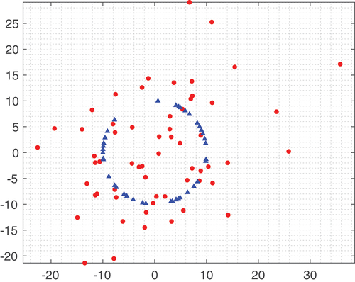
In this section, we analyze an example to show the superiority of geo-constrained symmetric transformation in estimating the transformation parameters. The circular feature is considered in this part. We do not give the conditional equations for circle features since: (1) It has been derived in detail by Hu et al. (2022); (2) It can be analogously formed as the ellipse feature, which will derived in the next section. The distribution of $100$ sampled points are shown in Figure 1. The true values of transformation parameters are $\tilde{s}=1.1$, $\tilde{\vartheta }=-{60}^{\circ }$ and $\tilde{\mathit{t}}=[-2030{]}^{\mathrm{T}}\mathrm{m}$. For the stochastic model, the covariance matrix is set to $\mathbf{\Sigma }={0.6}^2{\mathit{I}}_{200}$.

Figure 1. Distribution of points in the source frame (m): red points are the unconstrained points and blue triangles are the points on the circle.

Three schemes are employed in the experiments:

• Scheme 1: the traditional asymmetric transformation.

• Scheme 2: the traditional symmetric transformation method given in Section 2.

• Scheme 3: the proposed geo-constrained symmetric transformation method.

Note that each scheme can be implemented by many specific algorithms, which produce the same estimation results. To evaluate the performance the Schemes, the estimation errors of different parameters can be evaluated as

${\epsilon }_s=\left|\hat{s}-\tilde{s}\left|{\epsilon }_R=\right|arccos\left(\left(\mathrm{tr}\left(\hat{\mathbf{R}}\tilde{\mathbf{R}}\right)\right)-1\right)/2\right|{\epsilon }_t=\parallel \hat{\mathbf{t}}-\tilde{t}{\parallel }_2.$

Totally $100$ experiments are conducted, the following steps are followed in each experiment: (a) Generate $\mathbf{e}$ from the normal distribution $\mathbb{N}(\mathbf{0},{0.1}^2{\mathit{I}}_{200})$; (b) Form the observations $\mathit{X}=\tilde{X}+E_X$ and $\mathit{Y}=\tilde{\mathit{Y}}+{\mathit{E}}_Y$; (c) Perform the estimations with different schemes; (d) Record the estimation errors for each scheme.

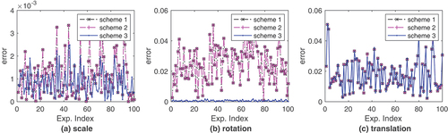
The estimation errors are shown in Figure 2, from which we can see that: (1) Scheme 1 and Scheme 2 produce nearly the same estimated parameters. This phenomenon has already been revealed by Xu et al. (2014). The difference between the asymmetric transformation and symmetric transformation depends on many factors such as the signal-noise-ratio, the transformation type and the correlations. As shown by Hu and Fang (2023), the difference would become significant if the observations are correlated. (2) In general, Scheme 3 has better performances (particularly the rotations) than the other two schemes: for the scale, Scheme 3 outperforms the other two schemes $64$ times out of $100$ experiments; for the rotation, Scheme 3 always outperforms the other two schemes; for the translation, these three schemes produces the similar results and do not show apparent differences. Therefore, the geo-constrained symmetric transformation is more appropriate in estimating the transformation parameters if the spatial information is available.

Figure 2. Estimation errors for three types of parameters (i.e. scale, rotation and translation) in $100$ experiments.

One would ask whether it is possible to apply such a method in transforming the newly collected points. We would analyze it in two aspects: (1) The consideration of available geometric constraints is essential as it can improve the estimated transformation parameters. (2) The consideration of the errors of source frame depends on the practitioner. In general, the purpose of the transformation only involving the common points shall be understood as adjusting the network configuration and the nuisance transformation parameters cannot be of direct use (Hu, Fang, and Kutterer 2023). It seems inappropriate to use them to transform non-common points as these points do not participate in the estimation process and should not be treated a posteriori (Kotsakis, Vatalis, and Sansò 2014; Li et al. 2013). In summary, a simplified version (taking ${\mathit{E}}_{\mathit{X}}=\mathbf{0}$) of our method has the potential to be applied to the point cloud registration problems (Ning et al. 2023; Wang et al. 2022a, 2022b, 2021, 2023b; Zhang et al. 2023).

5. Experiment analysis: point determination

In this section, we provide an example to illustrate the superiority of the geo-constrained symmetric transformation versus the traditional symmetric transformation in the point location determination. The geometric constraint considered here is the ellipse constraint, frequently occurring in real-life scenarios (Augustyn, Kampik, and Musioł 2023; Chen, Rottensteiner, and Heipke 2021; Ramos, Janeiro, and Radil 2009; Tao et al. 2023). As we have discussed before, the example compares the estimated point locations rather than the transformation parameters.

5.1. Ellipse constraints

We first show how to form the conditional model of the ellipse. The algebraic equation of the ellipse reads

(30) ${\tilde{z}}_{\mathit{i}}^{\mathrm{T}}\mathit{\nu }=1\mathrm{for}\mathit{i}\in \mathcal{G},$(30)

where ${\tilde{z}}_{\mathit{i}}=[{\tilde{x}}_{\mathit{i}}^2{\tilde{y}}_{\mathit{i}}^2{\tilde{x}}_{\mathit{i}}{\tilde{y}}_{\mathit{i}}{\tilde{x}}_{\mathit{i}}{\tilde{y}}_{\mathit{i}}{]}^{\mathrm{T}}$; and $\mathit{\nu }$ represents the $5$-vector of unknown algebraic coefficients. Choosing five points $\{i_1,i_2,i_3,i_4,i_5\}\subseteq \mathcal{G}$ we have

(31) $\tilde{L}\mathit{\nu }=1_5\Rightarrow \mathit{\nu }={\tilde{L}}^{-1}{1}_5,$(31)

where $\tilde{\mathit{L}}=[{\tilde{z}}_{i_1}{\tilde{z}}_{i_2}{\tilde{z}}_{i_3}{\tilde{z}}_{i_4}{\tilde{z}}_{i_5}{]}^{\mathrm{T}}$. For the rest points, we can have $(n_r-5)$ condition equations

(32) $\mathit{f}\left(\mathbf{\ell }-e_{\mathrm{\ell }}\right)=\left[\begin{array}{c}\cdots \\ {\left({\tilde{\mathit{L}}}^{-1}{\mathbf{1}}_5\right)}^{\mathrm{T}}{\tilde{z}}_{\mathit{i}}-1\\ \cdots \end{array}\right]=0\mathrm{for}\mathit{i}\in \mathcal{G}\mathrm{\setminus }\left\{i_1,i_2,i_3,i_4,i_5\right\}.$(32)

Therefore, the conditional model for the ellipse has been established and other conics with algebraic form can be formulated similarly.

With the ellipse constraints, the form of $\mathrm{\partial }{f}_i/\mathrm{\partial }{\tilde{\mathrm{\ell }}}^{\mathrm{T}}$ is as follows:

• If $\mathit{k}\in \{i_1,i_2,i_3,i_4,i_5\}$, we have

(33) $\frac{\partial f_i}{\partial {\tilde{x}}_{\mathit{k}}}=\frac{\partial {\tilde{L}}^{-1}}{\partial {\tilde{x}}_{\mathit{k}}}{1}_5\text{T}{\tilde{z}}_{\mathit{i}}={\tilde{z}}_{\mathit{i}}^{\text{T}}\left(\frac{\partial {\tilde{L}}^{-1}}{\partial {\tilde{x}}_{\mathit{k}}}{1}_5\right)\frac{\partial f_i}{\partial {\tilde{y}}_{\mathit{k}}}={\left(\frac{\partial {\tilde{L}}^{-1}}{\partial {\tilde{y}}_{\mathit{k}}}{1}_5\right)}^{\text{T}}{\tilde{z}}_{\mathit{i}}={\tilde{z}}_{\mathit{i}}^{\text{T}}\left(\frac{\partial {\tilde{L}}^{-1}}{\partial {\tilde{y}}_{\mathit{k}}}{1}_5\right)$(33)

with

(34) $\frac{\partial {\tilde{L}}^{-1}}{\partial {\tilde{x}}_{\mathit{k}}}=-{\tilde{L}}^{-1}\frac{\partial \tilde{L}}{\partial {\tilde{x}}_{\mathit{k}}}{\tilde{L}}^{-1}\frac{\partial {\tilde{L}}^{-1}}{\partial {\tilde{y}}_{\mathit{k}}}=-{\tilde{L}}^{-1}\frac{\partial \tilde{L}}{\partial {\tilde{y}}_{\mathit{k}}}{\tilde{L}}^{-1},$(34)

where

(35) $\frac{\mathrm{\partial }\tilde{\mathit{L}}}{\mathrm{\partial }{\tilde{x}}_{\mathit{k}}}=\left[\begin{array}{ccccc}0& 0& 0& 0& 0\\ ⋮& ⋮& ⋮& ⋮& ⋮\\ 2{\tilde{x}}_{\mathit{k}}& 0& 1& 0& {\tilde{y}}_{\mathit{k}}\\ ⋮& ⋮& ⋮& ⋮& ⋮\\ 0& 0& 0& 0& 0\end{array}\right]\frac{\mathrm{\partial }\tilde{\mathit{L}}}{\mathrm{\partial }{\tilde{y}}_{\mathit{k}}}=\left[\begin{array}{ccccc}0& 0& 0& 0& 0\\ ⋮& ⋮& ⋮& ⋮& ⋮\\ 0& 2{\tilde{y}}_{\mathit{k}}& 0& 1& {\tilde{x}}_{\mathit{k}}\\ ⋮& ⋮& ⋮& ⋮& ⋮\\ 0& 0& 0& 0& 0\end{array}\right].$(35)

• If $\mathit{k}\in \mathcal{G}\mathrm{\setminus }\{i_1,i_2,i_3,i_4,i_5\}$, we have

(36) $\frac{\partial f_i}{\partial {\tilde{x}}_{\mathit{k}}}={({\tilde{L}}^{-1}{1}_4)}^{\text{T}}\left[2{\tilde{x}}_{\mathit{k}}010{\tilde{y}}_{\mathit{k}}\right]\frac{\partial f_i}{\partial {\tilde{y}}_{\mathit{k}}}={({\tilde{L}}^{-1}{1}_4)}^{\text{T}}\left[02{\tilde{y}}_{\mathit{k}}01{\tilde{x}}_{\mathit{k}}\right].$(36)

• If $\mathit{k}\in \{1,2,\cdots ,4\mathit{n}\}\mathrm{\setminus }\mathcal{G}$, we have

(37) $\frac{\mathrm{\partial }{f}_i}{\mathrm{\partial }{\tilde{x}}_{\mathit{k}}}=0\frac{\mathrm{\partial }{f}_i}{\mathrm{\partial }{\tilde{y}}_{\mathit{k}}}=0.$(37)

Then, the matrix ${\mathit{B}}_F$ can be formed.

5.2. Experiment setup

Now, a total of $30$ points are measured in two different systems, $20$ of which are constrained points (i.e. the points distributed in the circumference of an ellipse.) The index subset of the constrained points is

$\begin{array}{cc}\mathcal{G}& =\{1,3,4,5,8,10,11,14,15,16,\\ \mathit{\hspace{0.17em}}& 17,18,19,20,22,23,27,28,29,30\}.\end{array}$

The distribution of the true locations of these $30$ points in the source frame is shown in Figure 3 and the true coordinates in the source frame are listed in Table 1. By setting the true values $\mathit{s}=0.95$, $\mathit{\vartheta }={30}^{\circ }$ and $\mathit{t}=[1020{]}^{\mathrm{T}}$ m, the true coordinates $\tilde{\mathit{Y}}$ can be computed according to Equation (1)(1) $\begin{array}{cc}\mathit{\hspace{0.17em}}& \mathit{Y}-{\mathit{E}}_{\mathit{Y}}=(\mathit{X}-{\mathit{E}}_{\mathit{X}})\mathit{R}+{\mathbf{1}}_n{\mathit{t}}^{\mathrm{T}}\\ \mathit{\hspace{0.17em}}& \mathit{e}:=\mathrm{vec}([{\mathit{E}}_{\mathit{X}}{\mathit{E}}_{\mathit{Y}}])\sim (\mathbf{0},\mathbf{\Sigma }={\mathit{P}}^{-1}),\end{array}$(1) . For the stochastic model, the covariance matrix is set to

Figure 3. Distribution of points in the source frame (m): red points are the unconstrained points and blue triangles are the points on the ellipse.

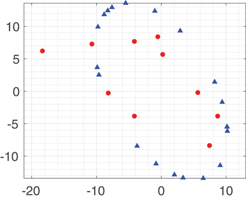
Table 1. True coordinates of sampled points in the source frame and the points marked with asterisk are those on the ellipse (m).

Point Num.	$\mathit{x}$-coordinate	$\mathit{y}$-coordinate	Point Num.	$\mathit{x}$-coordinate	$\mathit{y}$-coordinate
$1\ast$	$10.1489$	$-5.4997$	$16\ast$	$10.1940$	$-6.1526$
$2$	$-18.3449$	$6.2151$	$17\ast$	$8.2387$	$1.4328$
$3\ast$	$-3.7311$	$-8.4449$	$18\ast$	$-9.8870$	$3.6776$
$4\ast$	$6.4681$	$-13.4192$	$19\ast$	$2.9168$	$9.3125$
$5\ast$	$2.0221$	$-12.8723$	$20\ast$	$-7.6070$	$12.9265$
$6$	$0.2147$	$5.6767$	$21$	$-10.7091$	$7.2840$
$7$	$-0.5353$	$8.4009$	$22\ast$	$-8.8121$	$11.8293$
$8\ast$	$9.3943$	$-1.6783$	$23\ast$	$-5.4925$	$13.5805$
$9$	$5.6391$	$-0.2015$	$24$	$-4.1491$	$-3.8354$
$10\ast$	$3.3578$	$-13.3446$	$25$	$-8.1765$	$-0.2722$
$11\ast$	$10.1460$	$-5.4686$	$26$	$8.7003$	$-3.8340$
$12$	$-4.1512$	$7.6827$	$27\ast$	$-8.2597$	$12.4326$
$13$	$7.4415$	$-8.3681$	$28\ast$	$-9.7771$	$9.9254$
$14\ast$	$9.0875$	$-11.4352$	$29\ast$	$-0.9956$	$12.3626$
$15\ast$	$-9.6262$	$2.5193$	$30\ast$	$-0.8086$	$-11.1752$

(38) $\mathbf{\Sigma }={0.01}^2\left[\begin{array}{cc}{\mathit{Q}}_0& \mathbf{0}\\ \mathbf{0}& {\mathit{Q}}_0\end{array}\right]\mathrm{with}{\mathit{Q}}_0=\left[\frac{1}{1+5|i-j|}\right]$(38)

for testing the correlated case.

To adjust the network configuration, three schemes are employed:

• Scheme 1: the traditional asymmetric transformation.

• Scheme 2: the traditional symmetric transformation method given in Section 1.

• Scheme 3: the proposed geo-constrained symmetric transformation method with

  ${\mathcal{G}}_1=\{1,3,4,5,8,10,11,14,15,16\}.$

• Scheme 4: the proposed geo-constrained symmetric transformation method with ${\mathcal{G}}_2=\mathcal{G}$.

Here, Scheme 3 and Scheme 4 use the same set of points for transformation, but they utilize different spatial information. More specifically, Scheme 3 only regards $10$ points belong to an ellipse while Scheme 4 considers the constraints on $20$ points. The purpose of designing these two schemes is to show the effects of partially missing spatial information on the point determinations.

To evaluate the statistical performance, we have conducted $500$ repeated experiments. In each experiment, the following steps are followed: (a) Generate $\mathit{e}$ from the normal distribution $\mathbb{N}(\mathbf{0},\mathbf{\Sigma })$; (b) Form the observations $\mathit{X}=\tilde{\mathit{X}}+{\mathit{E}}_X$ and $\mathit{Y}=\tilde{\mathit{Y}}+{\mathit{E}}_Y$; (c) Compute the point locations with four schemes and record the discrepancy vectors by subtracting the true locations from the estimated locations.

5.3. Result analysis

After performing the computations, the two-dimensional confidence ellipses with a confidence probability $0.95$ for the three schemes in the source frame are shown in Figure 4. The confidence ellipse is determined with the eigenvalues and eigenvectors of the sample covariance matrix computed by the discrepancy vectors (Coe 2009; Zaminpardaz and Teunissen 2022). In addition, we have computed the root-mean-square errors (RMSEs) for these three schemes. Since the data are two-dimensional, the $\mathit{x}$- and $\mathit{y}$-directions are computed separately. For example, if the discrepancy series of $\mathit{k}$-th point in $\mathit{x}$-direction computed by Scheme 1 is $\{b_{x,1}^k,\cdots ,b_{x,500}^k\}$, the corresponding RMSE is ${\sum }_{i=1}^{500}(b_{x,i}^k{)}^2/500$. Furthermore, we have calculated the percentage of RMSE improvements (e.g. [Scheme 1 $-$ Scheme 2]/Scheme 1, [Scheme 1 $-$ Scheme 3]/Scheme 1, and [Scheme 1 $-$ Scheme 4]/Scheme 1), see Figure 5. It is worth noting that we do not present the results in the target frame as the symmetric transformation ensures the same configuration for both frames. Therefore, all the conclusions also hold for the estimated locations in the target frame.

Figure 4. Confidence ellipses of different points in the source frame (m). Black solid line, red solid line, blue dash-dotted line and magenta dashed line represent Scheme 1, Scheme 2, Scheme 3, and Scheme 4, respectively. Black circle is the zero point.

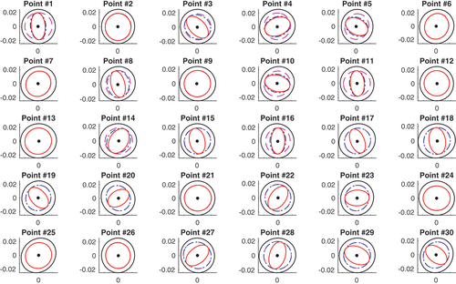
Figure 5. Percentage (%) of the improvement of RMSEs at different points. Red circle and blue plus sign represent Scheme 2 and Scheme 3, respectively.

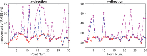
From the results we can see that: (1) The confidence ellipses of Scheme 1 are apparently bigger than those of the other three schemes, which shows the statistical inefficiency of asymmetric transformation in terms of point determination. (2) The confidence ellipses of Scheme 3 and Scheme 4 for all the points are either completely contained within or coincide with that of Scheme 2. This indicates that our proposed method does improve the statistical performance. (3) The accuracy improvements are more significant for the points ${\mathcal{G}}_1$ with Scheme 3 and for points ${\mathcal{G}}_2$ with Scheme 4. This suggests that the improvement is more pronounced for the points that are explicitly constrained. (4) Recalling the distribution of the points, the improvements gained by incorporating the geometric information primarily lie in the radial direction. In other words, the minor axis of the confidence ellipses produced by the geo-constrained symmetric transformation roughly aligns the normal of the geometric feature. (4) In terms of the RMSEs, the maximum improvements in $\mathit{x}$-direction are $29.48\mathrm{\%}$, $53.97$% and $58.78\mathrm{\%}$ for Scheme 2, Scheme 3 and Scheme 4, respectively; the maximum improvements in $\mathit{y}$-direction are $28.28\mathrm{\%}$, $45.98$ and $53.95\mathrm{\%}$ for Scheme 2, Scheme 3 and Scheme 4, respectively. Thus, the improvements by incorporating the geometric constraints are significant. We note that the maximum improvement in a specific direction can exceed such a ratio since the minor axis of the confidence ellipses does not coincide with the direction of $\mathit{x}$- or $\mathit{y}$-axis.

Therefore, in this example, we have shown the superiority of the geo-constrained symmetric transformation: (1) The RMSE of the point determination can be improved, and the increase can even beyond $50\mathrm{\%}$. (2) Incorporating more geometric information can provide more reliable results.

6. Concluding remarks

In this contribution, the symmetric transformation with geometric constraints is discussed. The combined model integrates the geometrical constraints and the symmetric transformation relation. The effects on the point determination are obtained by formulating the geometric constraints as conditional equations. Therefore, a modified scheme of the traditional symmetric transformation algorithm is proposed to ensure geometric constraint satisfaction. Taking the two-dimensional similarity transformation and the ellipse constraints, for example, we show that our method can significantly improve the statistical accuracy of point location in real applications, with an improvement of over 50% in terms of the RMSE. Though only the two-dimensional case is presented, the three-dimensional case can be naturally extended. The analysis and formulations in Section 3 are all valid, and the only difference is the form of coefficient matrices.

As the geometric constraints can significantly improve the estimated transformation parameters, we will apply it to point cloud registration problem. In addition, the three-dimensional cases such as point positioning and stereo-image matching will be researched.

Disclosure statement

No potential conflict of interest was reported by the author(s).

Data availability statement

All data analyzed during this study are included in this published article.

Additional information

Funding

This research was funded by the National Natural Science Foundation of China [42174049; 42274007] and the Special Fund of Hubei Luojia Laboratory [No. 220100003].

Notes on contributors

Wenxi Zhan

Wenxi Zhan is an M.S. degree candidate at Wuhan University. Her research interests include spatial statistics and geographical information analysis.

Wenxian Zeng

Wenxian Zeng received her Ph.D. degree in geodesy from Wuhan University in 2013. She has been a full professor since 2023. Her research interests include adjustment theory, methods and applications.

Yibin Yao

Yibin Yao is a professor at the School of Geodesy and Geomatics at Wuhan University. He received his Ph.D. degree in Geodesy and Surveying Engineering from Wuhan University in 2004. His current research interest is in the GNSS ionospheric, atmospheric, and meteorological studies and high-precision GNSS data processing.

Xing Fang

Xing Fang received a Diplom degree and PH.D. degree in the geodetic institute at Leibniz University of Hanover, Germany in 2007 and 2011. He was a post-doctoral fellow at the Ohio State University, USA from 2015 to 2017. He got his current position at Wuhan University as Associate Professor in 2013 and his main research includes parameter estimation and robust statistics.

Dawei Li

Dawei Li received his Ph.D. degree in geodesy from Wuhan University in 2013. He was a post-doctoral fellow at the Wuhan University from 2013 to 2017. He got his current position at Wuhan University as Lecturer in 2017. His current research interest is in geodesy data processing.

References

- Augustyn, J., M. Kampik, and K. Musioł. 2023. “On Determination of the Complex Voltage Ratio Using the Ellipse-Fitting Algorithm in the Case of an Ill-Conditioned Scattering Matrix.” Measurement 216:112935. https://doi.org/10.1016/j.measurement.2023.112935.
- Cai, B., Z. Shao, S. Fang, X. Huang, Y. Tang, M. Zheng, and H. Zhang. 2022. “The Evolution of Urban Agglomerations in China and How it Deviates from Zipf’s Law.” Geo-Spatial Information Science 1–11. https://doi.org/10.1080/10095020.2022.2083527.
- Chang, G., T. Xu, and Q. Wang. 2018. “M-Estimator for the 3D Symmetric Helmert Coordinate Transformation.” Journal of Geodesy 92 (1): 47–58. https://doi.org/10.1007/s00190-017-1043-9.
- Chen, L., F. Rottensteiner, and C. Heipke. 2021. “Feature Detection and Description for Image Matching: From Hand-Crafted Design to Deep Learning.” Geo-Spatial Information Science 24 (1): 58–74. https://doi.org/10.1080/10095020.2020.1843376.
- Chen, J., and J. Wang. 2009. “Orbit Fitting Based on Helmert Transformation.” Geo-Spatial Information Science 12 (2): 95–99. https://doi.org/10.1007/s11806-009-0236-7.
- Coe, D. 2009. “Fisher Matrices and Confidence Ellipses: A Quick-Start Guide and Software.” arXiv Preprint arXiv: 0906.4123.
- Dong, J., S. Li, L. Huang, J. He, W. Jiang, F. Ren, Y. Wang, J. Sun, and H. Zhang. 2022. “Identification of International Trade Patterns of Agricultural Products: The Evolution of Communities and Their Core Countries.” Geo-Spatial Information Science 1–15. https://doi.org/10.1080/10095020.2022.2122875.
- Fang, X. 2011. “Weighted Total Least Squares Solutions for Applications in Geodesy.” PhD diss., Hannover: Gottfried Wilhelm Leibniz Universität Hannover.
- Fang, X. 2013. “Weighted Total Least Squares: Necessary and Sufficient Conditions, Fixed and Random Parameters.” Journal of Geodesy 87 (8): 733–749. https://doi.org/10.1007/s00190-013-0643-2.
- Fang, X. 2014a. “On Non-Combinatorial Weighted Total Least Squares with Inequality Constraints.” Journal of Geodesy 88:805–816. https://doi.org/10.1007/s00190-014-0723-y.
- Fang, X. 2014b. “A Structured and Constrained Total Least-Squares Solution with Cross-Covariances.” Studia Geophysica Et Geodaetica 58 (1): 1–16. https://doi.org/10.1007/s11200-012-0671-z.
- Fang, X. 2015. “Weighted Total Least-Squares with Constraints: A Universal Formula for Geodetic Symmetrical Transformations.” Journal of Geodesy 89 (5): 459–469. https://doi.org/10.1007/s00190-015-0790-8.
- Fang, X., Y. Hu, W. Zeng, and O. Akyilmaz. 2022. “Weighted Least-Squares Fitting of Circles with Variance Component Estimation.” Measurement 205:112132. https://doi.org/10.1016/j.measurement.2022.112132.
- Förstner, W., and B. Wrobel. 2016. Photogrammetric Computer Vision. Switzerland: Springer International Publishing.
- Frahm, J., J. Heinly, E. Zheng, E. Dunn, P. Fite-Georgel, and M. Pollefeys. 2013. “Geo-Registered 3D Models from Crowdsourced Image Collections.” Geo-Spatial Information Science 16 (1): 55–60. https://doi.org/10.1080/10095020.2013.774103.
- Houshiar, H., J. Elseberg, D. Borrmann, and A. Nüchter. 2015. “A Study of Projections for Key Point Based Registration of Panoramic Terrestrial 3D Laser Scan.” Geo-Spatial Information Science 18 (1): 11–31. https://doi.org/10.1080/10095020.2015.1017913.
- Hu, Y., and X. Fang. 2023. “Linear Estimation Under the Gauss–Helmert Model: Geometrical Interpretation and General Solution.” Journal of Geodesy 97 (5): 44. https://doi.org/10.1007/s00190-023-01737-x.
- Hu, Y., X. Fang, and H. Kutterer. 2023. “Center Strategies for Universal Transformations: Modified Iteration Policy and Two Alternative Models.” GPS Solutions 27 (2): 92. https://doi.org/10.1007/s10291-023-01419-3.
- Hu, Y., X. Fang, Y. Qin, and O. Akyilmaz. 2022. “Weighted Geometric Circle Fitting for the Brogar Ring: Parameter-Free Approach and Bias Analysis.” Measurement 192:110832. https://doi.org/10.1016/j.measurement.2022.110832.
- Hu, Y., X. Fang, W. Zeng, and H. Kutterer. 2023. “Multi-Frame Transformation with Variance Component Estimation.” IEEE Transactions on Geoscience & Remote Sensing 61:1–10. https://doi.org/10.1109/TGRS.2023.3302322.
- Kanatani, K. 1994. “Analysis of 3-D Rotation Fitting.” IEEE Transactions on Pattern Analysis & Machine Intelligence 16 (5): 543–549. https://doi.org/10.1109/34.291441.
- Kotsakis, C., A. Vatalis, and F. Sansò. 2014. “On the Importance of Intra-Frame and Inter-Frame Covariances in Frame Transformation Theory.” Journal of Geodesy 88 (12): 1187–1201. https://doi.org/10.1007/s00190-014-0753-5.
- Leick, A., L. Rapoport, and D. Tatarnikov. 2015. GPS satellite surveying. Hoboken, New Jersey: John Wiley & Sons, Inc.
- Li, B., Y. Shen, X. Zhang, C. Li, and L. Lou. 2013. “Seamless Multivariate Affine Error-In-Variables Transformation and Its Application to Map Rectification.” International Journal of Geographical Information Science 27 (8): 1572–1592. https://doi.org/10.1080/13658816.2012.760202.
- Mercan, H., O. Akyilmaz, and C. Aydin. 2018. “Solution of the Weighted Symmetric Similarity Transformations Based on Quaternions.” Journal of Geodesy 92 (10): 1113–1130. https://doi.org/10.1007/s00190-017-1104-0.
- Ning, E., C. Wang, H. Zhang, X. Ning, and P. Tiwari. 2023. “Occluded Person Re-Identification with Deep Learning: A Survey and Perspectives.” Expert Systems with Applications 122419. https://doi.org/10.1016/j.eswa.2023.122419.
- Ramos, P., F. Janeiro, and T. Radil. 2009. “Comparison of Impedance Measurements in a DSP Using Ellipse-Fit and Seven-Parameter Sine-Fit Algorithms.” Measurement 42 (9): 1370–1379. https://doi.org/10.1016/j.measurement.2009.05.005.
- Rao, C. R., H. Toutenburg, and C. Heumann. 2008. Linear Models and Generalizations: Least Squares and Alternatives. Berlin, Heidelberg: Springer.
- Schaffrin, B., and Y. A. Felus. 2008. “On the Multivariate Total Least-Squares Approach to Empirical Coordinate Transformations. Three Algorithms.” Journal of Geodesy 82 (6): 373–383. https://doi.org/10.1007/s00190-007-0186-5.
- Tao, L., R. Xia, J. Zhao, T. Zhang, Y. Li, Y. Chen, and S. Fu. 2023. “A High-Accuracy Circular Hole Measurement Method Based on Multi-Camera System.” Measurement 207:112361. https://doi.org/10.1016/j.measurement.2022.112361.
- Tran, D., J. Nocquet, N. Luong, and D. Nguyen. 2023. “Determination of Helmert Transformation Parameters for Continuous GNSS Networks: A Case Study of the Géoazur GNSS Network.” Geo-Spatial Information Science 26 (1): 125–138. https://doi.org/10.1080/10095020.2022.2138569.
- Umeyama, S. 1991. “Least-Squares Estimation of Transformation Parameters Between Two Point Patterns.” IEEE Transactions on Pattern Analysis & Machine Intelligence 13 (4): 376–380. https://doi.org/10.1109/34.88573.
- Wang, C., X. Ning, W. Li, X. Bai, and X. Gao. 2023. “3D Person Re-Identification Based on Global Semantic Guidance and Local Feature Aggregation.” IEEE Transactions on Circuits and Systems for Video Technology 1–1. https://doi.org/10.1109/TCSVT.2023.3328712.
- Wang, C., X. Ning, L. Sun, L. Zhang, W. Li, and X. Bai. 2022. “Learning Discriminative Features by Covering Local Geometric Space for Point Cloud Analysis.” IEEE Transactions on Geoscience & Remote Sensing 60:1–15. https://doi.org/10.1109/TGRS.2022.3170493.
- Wang, C., C. Wang, W. Li, and H. Wang. 2021. “A Brief Survey on RGB-D Semantic Segmentation Using Deep Learning.” Displays 70:102080. https://doi.org/10.1016/j.displa.2021.102080.
- Wang, C., H. Wang, X. Ning, S. Tian, and W. Li. 2022. “3D Point Cloud Classification Method Based on Dynamic Coverage of Local Area.” Journal of Software 34 (4): 1962–1976. (in Chinese with English abstract).
- Wang, Y., M. Wang, Y. Zhu, and X. Long. 2024. “Low Frequency Error Analysis and Calibration for Multiple Star Sensors System of GaoFen7 Satellite.” Geo-Spatial Information Science 27 (1): 82–94. https://doi.org/10.1080/10095020.2022.2100284.
- Wang, B., Z. Zhao, Y. Chen, and J. Yu. 2023. “A Novel Robust Point Cloud Fitting Algorithm Based on Nonlinear Gauss–Helmert Model.” IEEE Transactions on Instrumentation and Measurement 72:1–12. https://doi.org/10.1109/TIM.2023.3239630.
- Xu, P., J. Liu, W. Zeng, and Y. Shen. 2014. “Effects of Errors-In-Variables on Weighted Least Squares Estimation.” Journal of Geodesy 88 (7): 705–716. https://doi.org/10.1007/s00190-014-0716-x.
- Yoshimura, R., H. Date, S. Kanai, R. Honma, K. Oda, and T. Ikeda. 2016. “Automatic Registration of MLS Point Clouds and SfM Meshes of Urban Area.” Geo-Spatial Information Science 19 (3): 171–181. https://doi.org/10.1080/10095020.2016.1212517.
- Zaminpardaz, S., and P. Teunissen. 2022. “On the Computation of Confidence Regions and Error Ellipses: A Critical Appraisal.” Journal of Geodesy 96 (2): 10. https://doi.org/10.1007/s00190-022-01596-y.
- Zhang, H., C. Wang, S. Tian, B. Lu, L. Zhang, X. Ning, and X. Bai. 2023. “Deep Learning-Based 3D Point Cloud Classification: A Systematic Survey and Outlook.” Displays 79:102456. https://doi.org/10.1016/j.displa.2023.102456.
- Zhu, Q., X. Guo, Z. Li, and D. Li. 2022. “A Review of Multi-Class Change Detection for Satellite Remote Sensing Imagery.” Geo-Spatial Information Science 1–15. https://doi.org/10.1080/10095020.2022.2128902.