Research on multiscale OpenStreetMap in China: data quality assessment with EWM-TOPSIS and GDP modeling

ABSTRACT

OpenStreetMap (OSM) is a voluntary platform designed to provide free and up-to-date geographic data. Since OSM is based on multisource geographic data provided by the public, the quality of the data has become a concern of researchers. In this study, a unified measure for evaluating OSM data quality was constructed, and the entropy weight method (EWM) and Technique for Order Performance by Similarity to Ideal Solution (TOPSIS) model were used to evaluate the quality of multiscale OSM data in China from 2014 to 2020. In addition to evaluating the data quality, the use of OSM data quality index factors in economic modeling at different spatial scales in China was explored by using a geographic information system (GIS) analysis method and a geographically and temporally weighted regression (GTWR) model. Four machine learning models, SVM, RF, XGBoost and CatBoost, were used to simulate the grid-scale GDP, and the effectiveness of these simulations was discussed. The results showed that (1) the weights of OSM data quality indicator factors vary across different spatial scales. (2) From 2014 to 2020, the quality of national-scale OSM data first increased, then decreased and then gradually stabilized. In addition, the quality of OSM data at the provincial and municipal scales is significantly different, and the distribution is affected by the population and geographical environment. (3) Over time, the spatial clustering characteristics of OSM data quality at different spatial scales in China has continuously strengthened. In addition, the quality of Chinese OSM data displays obvious local spatial autocorrelation characteristics, which are dominated by H-H clustering and L-L clustering. (4) The GTWR model performs well in predicting and revealing the spatiotemporal correlation characteristics between GDP and OSM data quality indicators at the provincial and municipal scales in China. The correlations increase with decreasing spatial scale (provincial to municipal). Moreover, the GDP modeling ability is better in economically underdeveloped Northwest China and economically developed East China. (5) Four machine learning models coupled with road network length completeness, relative linear density, road name attribute completeness, POI name attribute completeness, road network accuracy, road network update frequency, POI update frequency, topological consistency and directional similarity yielded the best grid-scale GDP simulation values. Notably, the CatBoost model provided the best accuracy, and the results further verified that it is feasible to use the proposed OSM data quality index system to predict the regional economic development level in China.

KEYWORDS:

• OpenStreetMap (OSM)
• data quality
• economic modeling
• geographically and temporally weighted regression (GTWR)
• machine learning
• China

1. Introduction

The concept of volunteered geographic information (VGI) was first proposed by Goodchild (2007) and refers to the voluntary contribution of geographic data by the public. It is called volunteer geographic information because it is provided free of charge by the public (See et al. 2016). OpenStreetMap (OSM) is considered one of the most well-known VGI projects (Goodchild and Li 2012).

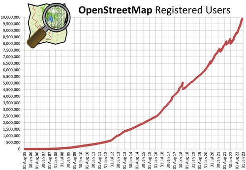
OSM, launched in 2004, is a collaborative mapping project aimed at providing world maps in the form of a freely available database of geographical features, which can be edited by anyone (Haklay and Weber 2008). With the rapid development of the OSM project, it has attracted increasing social and academic attention. As of January 2023, the number of registered users reached nearly 10 million (Figure 1), and this number is still growing rapidly worldwide. Compared with traditional geographic data, this VGI dataset is massive, heterogeneous, detailed and free, so it has attracted extensive attention from researchers (Neis and Zielstra 2014). At present, OSM research has been extended to many fields, such as urban expansion (Barrington-Leigh and Millard-Ball 2020; Zhan and Ukkusuri 2019), 3D urban modeling (Hadimlioglu and King 2019; Schellekens et al. 2014), robot navigation (Li et al. 2022), spatial queries (Chaves Carniel 2023), and disaster relief (Goldblatt, Jones, and Mannix 2020). Although OSM has certain advantages in public management and planning, OSM data are contributed by public volunteers, which has led to some uncertainty regarding the quality of these data (Nasiri et al. 2018; Senaratne et al. 2017). Notably, the data quality has a direct impact on the accuracy of the research results (Mooney and Morgan 2015). Therefore, before applying OSM data to specific projects or studies, it is necessary to understand and evaluate OSM data quality (Luo et al. 2019).

Figure 1. Number of registered OSM users (https://wiki.openstreetmap.org/wiki/Stats).

Quality assessments of VGI data are generally in accordance with the relevant regulations of the International Standards Organization (ISO) for data quality (Blower et al. 2015; Brodeur et al. 2019). Scholars from different countries and regions have proposed various evaluation methods and models, and the differences between these methods are mainly associated with the selection of reference data, quality elements and quantification (Degrossi et al. 2018; Fan et al. 2014; Klonner et al. 2021). VGI quality analysis methods are generally divided into two categories (Jacobs and Mitchell 2020; Muttaqien, Ostermann, and Lemmens 2018): analyses of the quality of OSM data without using any external data and comparisons of OSM data with external datasets (reference datasets), or so-called “intrinsic quality analysis” and “extrinsic quality analysis”, respectively. By selecting different quality elements as the basis for analysis, the VGI and reference data are matched and compared to intuitively obtain reliable quantitative VGI quality information. Commonly used reference data include officially published data, measured data and remote sensing image data (Barrington-Leigh, Millard-Ball, and Ali 2017; Hecht, Kunze, and Hahmann 2013; Jokar Arsanjani, Peter, et al. 2015; Zhou 2018). The selection of quality elements is mainly based on data completeness, positioning accuracy, etc (Borkowska and Pokonieczny 2022; Forghani and Reza Delavar 2014; Husen, Idris, and Ishak 2018). which are widely considered factors in most countries. However, the primary challenge in data quality evaluation lies in the selection of representative dimensions to assess data quality (Medeiros and Holanda 2019). Due to the multidimensional nature of data quality and varying requirements across different domains and industries, there are differences in how data quality is assessed, making it a complex and challenging concept to grasp and communicate. Therefore, in the context of spatial data quality analysis, the establishment of a unified metric is urgently needed. Such a unified measure can help users comprehend various aspects of OSM data quality, such as completeness, accuracy, and consistency, thus enabling the enhanced utilization of OSM data. For instance, Klonner et al. (2021) introduced the Sketch Map Tool, which aims to unify all the relevant necessary tools and utilizes OSM data for participatory mapping, employing a traffic-light-based system to communicate information about data quality and existing issues. In addition, it also facilitates OSM research, enhances collaboration and communication among community members, improves OSM data quality, and aids in further advancing the development and application of open maps (Barron, Neis, and Zipf 2014).

There are significant differences in the dimensions of spatial data quality evaluation indices and high uncertainty related to the number of evaluation objects selected. The analytical hierarchy process (AHP) and entropy weight method (EWM) are standard methods for the quantitative analysis of qualitative decision problems (Zyoud and Fuchs-Hanusch 2017). The AHP represents a weighting method that is highly subjective in its implementation (Rafi et al. 2020; Saaty 2013). It transforms human judgments into comparisons of the importance of several factors in a multilevel structure. However, in the application of the AHP, the evaluation objects and indices should be limited in number. The EWM is an objective weighting method that calculates weights based on available information as a measure of disorder in a system, and entropy is inversely proportional to the amount of information available (Zelany 1974). According to this rule, the information entropy level of each index can be obtained by using the inherent information provided by a given evaluation scheme. The smaller the entropy value is, the lower the degree of disorder, the greater the utility value of the information, and the greater the influence of indicators on the comprehensive evaluation. The evaluation of OSM data quality involves multiple indicators and factors, making quality assessment a typical quantitative multiattribute decision-making problem that requires effective evaluation methods. The Technique for Order Performance by Similarity to Ideal Solution (TOPSIS) method is widely used in multiobjective decision analysis and evaluation, and it is known for its computational convenience and scientifically rational outcomes (Jahanshahloo, Hosseinzadeh Lotfi, and Izadikhah 2006). It is currently widely applied across various domains for decision-making and evaluation purposes (Borkowska, Bielecka, and Pokonieczny 2023). TOPSIS is based on the idea that optimal performance corresponds to the shortest distance from a positive ideal solution and the greatest distance from a negative ideal solution (Zhu, Tian, and Yan 2020). Additionally, the TOPSIS method possesses several advantages (Shabani, Masoumi, and Rezaei 2022; Zyoud and Fuchs-Hanusch 2017). Notably, there are no strict restrictions on or requirements for the quantity and selection of indicators. Thus, this method can comprehensively integrate information from various attributes, avoiding information loss. The method is relatively simple to implement, eliminating the need for complex mathematical modeling and optimization processes. Moreover, it yields relatively intuitive and reliable evaluation results that are easy to visualize. Considering these advantages, the EWM-TOPSIS model was used in this study to evaluate the OSM data quality.

Specifically, the objective of this study is to establish a unified metric for evaluating OSM data quality using the EWM-TOPSIS model. Through this approach, we not only analyze the OSM data quality at different spatial and temporal scales in China but also present the results in a readily understandable manner and provide a quantitative theoretical basis and reference for subsequent application products and research involving OSM data. In addition, the application of OSM data to support economic development in China is explored, and OSM data quality index factors are used as explanatory variables to reflect regional economic development levels at different spatial scales, thus providing an effective reference index for evaluating regional economic development.

The innovations and contributions of this paper are as follows. (1) An evaluation index system for OSM data quality in China is constructed, and the quality of OSM data at different spatial and temporal scales in China is systematically evaluated with the combined EWM-TOPSIS model. (2) A GTWR model is used to explore the contributions of OSM data quality indicators in economic modeling at the provincial and municipal scales in China, and a machine learning model is used to simulate GDP at the grid scale. The results show that it is feasible to use the OSM data quality index system to predict the regional economic development level.

The rest of this paper is organized as follows: in Section 2, the OSM data quality index system is constructed, the methods are introduced and the relevant research data sources are described; in Section 3, the experimental results are analyzed; the study is discussed in Section 4; and the conclusions are given in Section 5.

2. Materials and methods

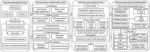
The research framework of this paper is presented in Figure 2. First, the OSM data quality evaluation index system in China was constructed from five dimensions: completeness, attribute accuracy, position accuracy, temporal accuracy, and logical consistency. Second, the weight of each index was determined using the EWM, and the TOPSIS method was applied to assess the OSM data quality in China. Then, spatial autocorrelation analysis was conducted to assess the spatial characteristics of the data at different scales. Finally, multiple models were used to explore the potential of OSM data quality indicators for use in economic modeling at different spatial scales in China.

Figure 2. Technical framework of this study.

2.1. OSM data quality evaluation index system

Satisfactory data quality is a basic requirement for any application of data. Quality evaluation models are simple and effective tools used to analyze and evaluate the quality of OSM data; specifically, OSM data can be compared with a reference dataset using appropriate quality indicators (Bright et al. 2018; H. Wu et al. 2021). According to the ISO definition, spatial data quality includes five indicators: completeness, attribute accuracy, position accuracy, temporal accuracy, and logical consistency (Brodeur 2001; Novack, Vorbeck, and Zipf 2022). An OSM data quality assessment can also follow ISO principles. Therefore, the following quality indicators are used to construct the OSM data quality evaluation index system in this study (Table 1).

Table 1. OSM data quality evaluation index system.

OSM data quality evaluation index system	Index layer	Index factor	Index type
	Completeness	Road network length completeness	+
		Relative linear density	-
	Attribute accuracy	Road name attribute completeness	+
		POI name attribute completeness	+
	Position accuracy	Road network accuracy	+
	Temporal accuracy	Road network update frequency	+
		POI update frequency	+
	Logical consistency	Topological consistency	-
		Directional similarity	-

“+” means that higher values are indicative of higher quality, and “-” means that lower values are indicative of higher quality.

2.1.1. Completeness

Data completeness, an ISO spatial data quality element, is primarily used to assess the effects of missing values in a dataset and serves as a fundamental measure in OSM research. In this paper, by comparing the coverage degree of the OSM dataset and reference dataset in a certain area, the road network length completeness and relative linear density were calculated and then used to reflect the completeness of the OSM data (Barrington-Leigh, Millard-Ball, and Ali 2017; Neis, Zielstra, and Zipf 2012). The corresponding formulas are as follows:

(1) $\mathit{Completenes}{s}_{\mathit{RLC}}=\frac{\sum {\mathit{L}}_{\mathit{OSM}}}{L_{\mathit{Ref}}}\times 100\mathrm{\%}$(1)

(2) $\mathit{Completenes}{s}_{\mathit{RLD}}=\left|\frac{{\mathit{L}}_{\mathit{Ref}}-\sum L_{\mathit{OSM}}}{\mathit{S}}\right|$(2)

where $\mathit{Completenes}{s}_{\mathit{RLC}}$ and $\mathit{Completenes}{s}_{\mathit{RLD}}$ represent road network length completeness and relative linear density, respectively, $\sum L_{\mathit{OSM}}$ represents the sum of the OSM road network length at each spatial scale, $L_{\mathit{Ref}}$ represents the actual road length of the reference data, and $\mathit{S}$ represents the area.

2.1.2. Attribute accuracy

Attribute accuracy refers to the accuracy or certainty of the attribute information associated with geographic data objects. Attribute data reflect the attributes of things, describe the attribute characteristics of data spatial elements and are an important part of geographic data. In the OSM dataset, the name attribute is the most frequently used attribute and the most important attribute in the evaluation process (Wang et al. 2013), so evaluating the name attribute is representative. Therefore, based on the road and POI names as representative attributes used to assess the OSM data attribute accuracy, the name attribute accuracy can be obtained from the following formula (Borkowska and Pokonieczny 2022):

(3) $\mathit{Attribute}\mathit{accurac}{y}_{\mathit{Name}}=\frac{\mathit{OS}{\mathit{M}}_{\mathit{Exist}\mathit{name}}}{\mathit{OS}{M}_{\mathit{All}}}\times 100\mathrm{\%}$(3)

where $\mathit{Attribute}\mathit{accurac}{y}_{\mathit{Name}}$ represents road or POI name attribute completeness and the value ranges from 0 to 100%, with 0% indicating that there are no OSM data in the area and 100% indicating that the name attribute accuracy has reached a maximum in that area.

2.1.3. Position accuracy

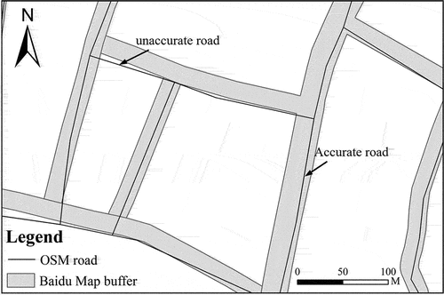
Position accuracy, which is the degree of geographic location deviation between the elements in the dataset to be evaluated and the elements in the reference dataset, is particularly important for spatial data and is often indicative of whether the data can be effectively used (Shan et al. 2023; Zhang, Leung, and Ma 2019). Line buffer overlay analysis can be used to effectively evaluate the position accuracy of line elements, as suggested by Goodchild and Hunter (Bright et al. 2018; Elias et al. 2020; Zhang et al. 2015). According to Zheng and Zheng (2014), OSM data within 20 m of Baidu Maps data can be regarded as accurate (Figure 3). Therefore, it is necessary to set a 20 m buffer for Baidu Maps data and overlay the established buffer layer with OSM road network data for analysis to calculate the percentage of road network overlap.

(4) $\mathit{Road}\mathit{network}\mathit{accurac}{y}_{\mathit{OSM}}=\frac{{\mathit{L}}_{\mathit{OSM}}\cap \mathit{Buffe}{r}_{\mathit{Ref}}}{L_{\mathit{OSM}}}\times 100\mathrm{\%}$(4)

Figure 3. Position accuracy evaluation.

2.1.4. Temporal accuracy

For OSM data, temporal accuracy serves as a critical metric for assessing the correspondence between the OSM dataset and real-world changes (Minghini and Frassinelli 2019), which is chiefly manifested through two key indicators in this paper: road network update frequency and POI update frequency (Girres and Touya 2010).

(5) $\mathit{Temporal}\mathit{accuracy}=\frac{\mathit{Numbe}{\mathit{r}}_{\mathit{OS}{\mathit{M}}_{\mathit{Edit},\mathit{t}+1}}-\mathit{Numbe}{r}_{\mathit{OS}{\mathit{M}}_{\mathit{Edit},\mathit{t}}}}{\mathit{Numbe}{r}_{\mathit{OS}{\mathit{M}}_{\mathit{Edit},\mathit{t}}}}\times 100\mathrm{\%}$(5)

where $\mathit{Temporal}\mathit{accuracy}$ represents the road network or POI update frequency, $\mathit{t}$ is the year and $\mathit{t}=2014,2015,\dots ,2020$, and $\mathit{Numbe}{r}_{\mathit{OS}{\mathit{M}}_{\mathit{Edit},\mathit{t}}}$ represents the number of times the road network or POI was edited in the t-th year. When $\mathit{Numbe}{r}_{\mathit{OS}{\mathit{M}}_{\mathit{Edit},\mathit{t}+1}}$ is less than $\mathit{Numbe}{r}_{\mathit{OS}{\mathit{M}}_{\mathit{Edit},\mathit{t}}}$, $\mathit{Temporal}\mathit{accuracy}$ is equal to 0.

2.1.5. Logical consistency

Logical consistency describes the credibility of the topology and relationships among datasets (Zielstra and Hochmair 2011). The logical consistency of OSM data is mainly reflected by directional similarity and topological consistency (Hashemi and Abbaspour 2015; Jokar Arsanjani, et al. 2015; Xu et al. 2017). Directional similarity is used to evaluate the similarity between OSM data and reference data in terms of direction and is realized by calculating the angle between the coordinates of the first and end points of OSM roads and Baidu Map roads and the x-axis direction and then calculating the angle difference between the two types of roads. Assuming the coordinates of the starting point and the ending point of a road (OSM or Baidu Maps) are $\left(x_0,\mathit{\hspace{0.17em}}{y}_0\right)$ and $\left(x_1,\mathit{\hspace{0.17em}}{y}_1\right)$, respectively, the formula for the bearing angle $\mathit{\delta }$ is as follows:

(6) $\mathit{\delta }=\mathit{arctan}\frac{y_1-y_0}{x_1-x_0}$(6)

In this process, the pairing of the OSM and Baidu Map datasets is established by employing OSM road data to generate grids and segmenting Baidu Map data to obtain common grid identifiers. The directional similarity between OSM data and Baidu Maps data is expressed by the difference between the two:

(7) $\mathit{Directional}\mathit{similarity}=\sum \left|{\delta }_{\mathit{OSM}}-{\delta }_{\mathit{ref}}\right|$(7)

Topological consistency describes the reliability of topological relations among OSM road data. Common polyline topology errors include overlap polylines, pseudonodes, and self-overlapping errors, by using ArcGIS software’s topology tools, and establishing topology rules including “Must not overlap polylines,” “Must not pseudonodes,” and “Must not self-overlap,” to identify topology errors. Topological consistency was calculated with the following formula:

(8) $\mathit{Topological}\mathit{consistenc}{y}_{\mathit{Road}}=\sum L_{\mathit{OSM}\mathit{topology}\mathit{error}}$(8)

2.2. Method

2.2.1. Weight determination

The EWM is used to determine index weights based on the statistics for an original dataset, thus ensuring the objectivity, authenticity and reliability of the evaluation process and effectively avoiding interference from human factors such as subjective weighting (Han et al. 2022), and the specific calculation steps are shown in Equations (9)(9) $P_{\mathit{ij}}=\frac{{\mathit{Y}}_{\mathit{ij}}}{{\sum }_{i=1}^m{Y}_{\mathit{ij}}}$(9) –(12(12) ${\omega }_j=\frac{1-e_j}{{\sum }_{j=1}^n(1-e_j)}$(12) ).

(9) $P_{\mathit{ij}}=\frac{{\mathit{Y}}_{\mathit{ij}}}{{\sum }_{i=1}^m{Y}_{\mathit{ij}}}$(9)

(10) $\mathit{K}=\frac{1}{\mathit{lnm}}$(10)

(11) $e_j=-\mathit{K}{\sum }_{i=1}^m{P}_{\mathit{ij}}\mathit{ln}{P}_{\mathit{ij}}$(11)

(12) ${\omega }_j=\frac{1-e_j}{{\sum }_{j=1}^n(1-e_j)}$(12)

where $P_{\mathit{ij}}$ represents the proportion of the $\mathit{j}$th index, $\mathit{m}$ represents the total number of samples, $e_j$ is the entropy value associated with the $\mathit{j}$th index, and ${\omega }_j$ represents the weight of the $\mathit{j}$th index. When $P_{\mathit{ij}}=0$, to make $\mathit{ln}{P}_{\mathit{ij}}$ meaningful, $\mathit{ln}{P}_{\mathit{ij}}=0$.

2.2.2. TOPSIS model

TOPSIS is a sorting method based on an ideal solution, and it is also known as the superior and inferior solution distance method. The objective is to transform a comprehensive evaluation problem into a problem involving the differences between evaluation objects based on a normalization matrix; then, the relative closeness between each index and the ideal solution is calculated with the optimal and inferior distances (Lin et al. 2020; Meng et al. 2018; Rafi et al. 2020). The specific steps are as follows.

Step 1: According to the selected indicators, establish the original data matrix $\mathit{R}$ of OSM data quality.

(13) $\mathit{R}=\left[\begin{array}{ccc}{r}_{11}& \cdots & r_{1\mathit{n}}\\ ⋮& \ddots & ⋮\\ r_{\mathit{m}1}& \cdots & r_{\mathit{mn}}\end{array}\right]$(13)

Step 2: Due to the inconsistent dimensions of the various indicators, standardize the units of the indicators to obtain the standardized matrix $\mathit{Y}{ }^{\mathrm{\prime }}$:

(14) $\mathrm{Positive}\mathrm{Index}+\mathit{\hspace{0.17em}}\mathit{Y}{ }^{\mathrm{\prime }}=\frac{{\mathit{r}}_{\mathit{mn}}-r_{\mathit{min}}}{r_{\mathit{max}}-r_{\mathit{min}}}$(14)

(15) $\mathrm{Negative}\mathrm{Index}-\mathit{\hspace{0.17em}}\mathit{Y}{ }^{\mathrm{\prime }}=\frac{{\mathit{r}}_{\mathit{max}}-r_{\mathit{mn}}}{r_{\mathit{max}}-r_{\mathit{min}}}$(15)

Step 3: Multiply the standardized matrix by the weights obtained with the EWM to obtain the weighted standardized matrix:

(16) $\mathit{Z}=\mathit{Y}{ }^{\mathrm{\prime }}\mathrm{\Omega }$(16)

Step 4: Determine the positive and negative ideal solutions $Z^{+}$ and $Z^{-}$ according to the weighted standardized matrix $\mathit{Z}$:

(17) $Z^{+}=\left\{\mathit{maxZ}\right\}=\left\{Z_1^{+},Z_2^{+},\dots Z_m^{+}\right\}$(17)

(18) $Z^{-}=\left\{\mathit{minZ}\right\}=\left\{Z_1^{-},Z_2^{-},\dots Z_m^{-}\right\}$(18)

Step 5: Calculate the Euclidean distance between each evaluation object and the positive and negative ideal solutions:

(19) $D^{+}=\sqrt{{\sum }_{j=1}^m{\left(Z-Z_j^{+}\right)}^2}$(19)

(20) $D^{-}=\sqrt{{\sum }_{j=1}^m{\left(Z-Z_j^{-}\right)}^2}$(20)

Step 6: Calculate the relative closeness between each evaluation object and the ideal solution:

(21) $\mathit{T}=\frac{D^{-}}{D^{+}+D^{-}}$(21)

where $\mathit{Y}{ }^{\mathrm{\prime }}$ is the standardized matrix, Ω is the index weight, $\mathit{m}$ is the number of quality measures, $Z^{+}\mathrm{and}{Z}^{-}$ are the positive and negative ideal solutions (in the context of the OSM data quality, they represent the set of highest and lowest values obtained in each evaluation index), respectively, $D^{+}\mathrm{and}{D}^{-}$ are the distances between the evaluation object (national, provincial, municipal, and grid) and the positive and negative ideal solutions, respectively, and $\mathit{T}$ is the relative closeness. The greater the closeness value is, the shorter the distance from the positive ideal solution and the farther the distance from the negative ideal solution the evaluation object is, that is, the higher the data quality level, and vice versa.

2.2.3. Spatial autocorrelation

Spatial autocorrelation reflects the degree of correlation between a certain geographical phenomenon or attribute value in a regional unit and the same phenomenon or attribute value in a neighboring regional unit (Griffith and Arbia 2010; Yao et al. 2023).

2.2.3.1. Global spatial autocorrelation

Global spatial autocorrelation describes the spatial agglomeration characteristics of the entire region of interest (Li, Wu, and Gao 2020; Wu et al. 2018). Moran’s I measure is the key indicator of global spatial autocorrelation, and global Moran’s I ranges from − 1 to 1, where values > 0 indicate a positive variable correlation with a tendency toward clustering and values < 0 indicate a spatially negative variable correlation with a tendency toward dispersion.

(22) $I_{\mathit{Global}}=\frac{n{\sum }_{x=1}^n{\sum }_{y=1}^n{W}_{\mathit{xy}}{T}_x{T}_y}{S_0{\sum }_{x=1}^n{T_x}^2}$(22)

(23) $S_0={\sum }_{x=1}^n{\sum }_{y=1}^n{W}_{\mathit{xy}}$(23)

where $I_{\mathit{Global}}$ represents the global Moran’s I, $\mathit{n}$ is the total number of spatial units studied, $T_x$ and $T_y$ represent the value $\mathit{T}$ of the OSM data quality in regions $\mathit{x}$ and $\mathit{y}$, respectively, and $W_{\mathit{xy}}$ is the spatial weight coefficient in regions $\mathit{x}$ and $\mathit{y}$, which is used to denote the neighboring relationship between spatial regions $\mathit{x}$ and $\mathit{y}$.

2.2.3.2. Local spatial autocorrelation

Local spatial autocorrelation mainly involves the specific characteristics of internal spatial agglomerations, thus differing from the global Moran’s I metric; additionally, the local spatial autocorrelation overcomes the issue that in the global Moran’s I approach, some local details are ignored (Ord and Getis 1995; Qiu et al. 2022). The formulas for the local Moran’s I statistic are as follows:

(24) $I_{\mathit{Local}}=\frac{T_x-\mathit{T}}{S_x^2}\cdot {\sum }_{y=1,y\ne x}^n{W}_{\mathit{xy}}\left(T_y-\mathit{T}\right)$(24)

(25) $S_x^2=\frac{{\sum }_{y=1,y\ne x}^n{\left(T_y-\mathit{T}\right)}^2}{\mathit{n}-1}-T^2$(25)

where $I_{\mathit{Local}}$ represents the local Moran’s I and $W_{\mathit{xy}}$ is an element of the spatial weight matrix $\mathit{W}$. The spatial weight matrix is the starting point of spatial statistics and testing models. The first-order adjacency matrix, which is the most widely used spatial adjacency matrix, considers that an adjacency relationship exists when regions $\mathit{x}$ and $\mathit{y}$ have a common edge (Zhou et al. 2017). Moreover, the first-order adjacency matrix expresses the boundary adjacency relationship between provinces and municipalities well. Therefore, the first-order adjacency matrix is selected in this paper to construct the spatial weight matrix. According to the calculation results, the agglomeration state can be divided into high-high clusters (H-H), low-low clusters (L-L), high-low clusters (H-L) and low-high clusters (L-H).

2.2.4. Geographically and temporally weighted regression

The geographically weighted regression (GWR) model emphasizes spatial nonstationarity and ignores temporal effects (Lu et al. 2022). The geographically and temporally weighted regression (GTWR) model is an extension of the GWR and is a local regression model in which spatial and temporal changes are considered, which can effectively reflect the evolutionary relationship of variables in time and space (Huang, Wu, and Barry 2010). The GTWR model is expressed as follows:

(26) $y_i={\beta }_0\left(u_i,v_i,t_i\right)+{\sum }_{k=1}^p{\beta }_k\left(u_i,v_i,t_i\right)X_{\mathit{ik}}+{\epsilon }_i,\mathit{i}=1,2,\dots ,\mathit{n}$(26)

where $\left(u_i,v_i,t_i\right)$ is point $\mathit{i}$ in time and space coordinates; $u_i,v_i,\mathrm{and}{t}_i$ represent the longitude, latitude and time information for point $\mathit{i}$; ${\beta }_0\left(u_i,v_i,t_i\right)$ is a constant; ${\beta }_k\left(u_i,v_i,t_i\right)$ is the $\mathit{k}$th regression coefficient of point $\mathit{i}$; and ${\epsilon }_i$ is the residual term of the model. ${ }^{{\beta }_i}$(regression coefficient) at sample point $\mathit{i}$ can be computed by the least-squares algorithm as:

(27) ${ }^{{\beta }_i}\left(u_i,v_i,t_i\right)={\left(\mathit{X}{\mathit{ }}^{\mathrm{\prime }}\mathit{W}\left(u_i,v_i,t_i\right)\mathit{X}\right)}^{-1}\mathit{X}{ }^{\mathrm{\prime }}\mathit{W}\left(u_i,v_i,t_i\right)y_i$(27)

where $\mathit{W}\left(u_i,v_i,t_i\right)$ is the space-time weight matrix and a Gaussian function is used as the weight function. The selection of bandwidth affects the determination of the space-time weights, and the AICc is adopted in this paper to adjust the bandwidth.

2.2.5. Machine learning models and evaluation criteria

This study utilized four machine learning algorithms, including Support Vector Machine (SVM), Random Forest (RF), Extreme gradient boosting (XGBoost), and Gradient boosting with categorical features support (CatBoost).

SVM is a kind of generalized linear classifier for data regression or classification based on supervised learning. The foundation of the SVM approach was established by Vapnik (1999), and Bray and Han (2004) introduced the first SVM model. RF concept was originally proposed by Breiman (2001), which is a parallel enhanced machine learning algorithm that combines the bagging method and the classification and regression tree (CART) model. XGBoost is a highly scalable, flexible, and versatile gradient boosting algorithm proposed by Chen and Guestrin (2016). This method reduces model overfitting by introducing regularization parameters, thereby improving the speed and efficiency of the model. CatBoost is an open-source machine learning library that was proposed by Yandex engineers in 2017 (Prokhorenkova et al. 2018). It is a machine learning method based on the gradient boosting decision tree (GBDT) approach. The algorithm mitigates the traditional gradient bias and prediction offset problems, thereby reducing the occurrence of overfitting and improving the accuracy and generalizability ability of the algorithm (Huang et al. 2019; Zhang, Zhao, and Zheng 2020).

Three commonly used statistical indicators are used to evaluate the accuracy and performance of the different machine learning models: the mean absolute error ($\mathit{MAE}$), root mean square error ($\mathit{RMSE}$), and coefficient of determination ($R^2$) (Despotovic et al. 2015).

(28) $\mathit{MAE}=\frac{1}{n}{\sum }_{i=1}^q\left|P_i-O_i\right|$(28)

(29) $\mathit{RMSE}=\sqrt{\frac{{\sum }_{i=1}^q{\left(P_i-O_i\right)}^2}{\mathit{n}}}$(29)

(30) $R^2=1-\frac{{\sum }_{i=1}^q{\left(O_i-P_i\right)}^2}{{\sum }_{i=1}^q{\left(O_i-\mathit{O}\right)}^2}$(30)

where $\mathit{q}$ is the total number of samples, $O_i$ is the actual value, $P_i$ is the estimated value, and $\mathit{O}$ is the average of all actual values $O_i$.

2.3. Data source

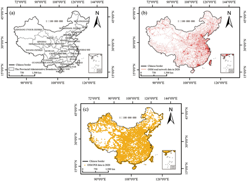
The vector boundary of the research area (Figure 4a) was obtained from the Resource and Environment Science and Data Center (https://www.resdc.cn/). OSM data are typically obtained in two ways. The first way involves selecting a specific area with a selection box and then downloading a corresponding geographic dataset on the official OSM website (https://www.openstreetmap.org/). The second way is to access free OSM data via the GeoFabrik and CloudMade download websites. The data have two formats: OSM-XML and shapefile. The latter is used in this study to download OSM data (all types of roads (Figure 4b), such as primary and secondary roads, and points of interest (POIs) (Figure 4c)) for China from CloudMade in shapefile format from 2014 to 2020.

Figure 4. (a) The vector boundary of the study area, (b) OSM road network data in 2020, (c) OSM POI data in 2020.

Baidu Maps (https://map.baidu.com/) is a relatively successful company in China, and the available data are highly complete and comprehensive and often used by the public for query and navigation tasks, with certain representative and authoritative data, which can be used as reference data. Roads and POIs in the two datasets were compared. Additional reference data, such as road mileage data, were collected from the China Statistical Yearbook and China City Statistical Yearbook from 2015 to 2021. Baidu Maps utilizes the BD-09 coordinate system, whereas the geographic data in the OSM dataset are from the World Geodetic System 1984 (WGS 84). Thus, ensuring spatial location consistency requires a series of coordinate conversions (Gao, Xu, and Li 2021; Xu et al. 2016). First, the BD-09 coordinate system was transformed into the Mars coordinate system (GCJ-02). Subsequently, the GCJ-02 coordinate system was further converted to the WGS 84 coordinate system. Finally, the “Projections and Transformations” tool in ArcGIS software was used to uniformly project the two types of data to the Universal Transverse Mercator (UTM) Zone 50 N.

The categorization discrepancies between OSM data and the reference dataset were considered; for example, the primary and secondary roads in OSM are classified based on the traffic volume, whereas Baidu Maps categorizes roads according to their administrative status, such as national, provincial, and county roads. Therefore, in this study, we compared and analyzed the categories with high similarity between the two datasets to obtain the final classification (Table 2).

Table 2. Corresponding relationships between OSM data and the reference data.

OSM tags	Reference dataset
Motorway, Motorway_link	Expressway
Trunk, Trunk_link	National roads
Primary, Primary_link	Provincial roads
Secondary, Secondary_link	County roads
Tertiary, Tertiary_link, Service, Living_street, Residential	Township roads
Unclassified, Track, Track_grade1–5	Village roads

3. Results

3.1. EWM-Based indicator weight calculation

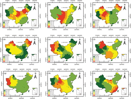
Due to the involvement of multiple spatial scales, including national, provincial, municipal, and grid scales, distinct indicators might exhibit divergent levels of significance and contribution. Consequently, we employed the EWM (Figure 2) for the computation of indicator weights concerning each specific spatial scale (Table 3). At the national, provincial, and municipal scales, the indicators “road network update frequency” and “POI update frequency” emerged as the most influential factors. However, at the grid scale, the indicator “road network accuracy” assumed utmost importance, constituting 45.40% of the entire indicator system weight.

Table 3. The weights of OSM data quality indicators at different scales.

Index factor	National	Provincial	Municipal	Grid
Road network length completeness	9.45%	18.48%	16.74%	15.37%
Relative linear density	9.78%	5.79%	0.79%	0.05%
Road name attribute completeness	11.26%	10.60%	10.89%	10.00%
POI name attribute completeness	7.52%	7.99%	11.38%	13.01%
Road network accuracy	10.11%	8.44%	9.65%	45.40%
Road network update frequency	12.73%	21.70%	22.40%	6.31%
POI update frequency	20.25%	19.75%	24.42%	9.70%
Topological consistency	12.32%	1.68%	0.47%	0.14%
Directional similarity	6.59%	5.58%	3.26%	0.02%

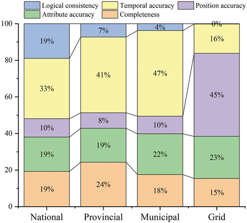
In addition, we explored the impact of different quality dimensions on OSM data quality at various spatial scales (Figure 5), and the results indicate significant variations in the weights of quality dimensions across different scales. Specifically, at the national scale, the weight of “temporal accuracy” is the highest (33%), followed by “completeness”, “attribute accuracy”, and “logical consistency”, with each of them having a weight of approximately 19%. As the spatial scale gradually decreases to the provincial and municipal scales, “temporal accuracy” becomes even more crucial, with weights of 41% and 47% respectively. However, at the more refined grid scale, “position accuracy” emerges as the predominant factor, accounting for 45% of the overall weight. This indicates the critical importance of accurate spatial information for data quality at smaller scales.

Figure 5. The weights of quality dimensions at different spatial scales.

3.2. OSM data quality analysis at multiple scales in China

Based on the OSM data quality evaluation index system constructed in this paper and combined with the EWM-TOPSIS model (Figure 2), the OSM data quality in China from 2014 to 2020 was obtained (Table 4 and Figure 6). The OSM data quality in China displayed a fluctuating trend over the years studied, with an initial increase followed by a decrease before eventually stabilizing, with the highest quality in 2017. A particular concern lies in the consistently low road name attribute completeness, which has remained at approximately 20% over the past seven years. Furthermore, we noted varying degrees of decrease in the relative linear density, road network accuracy, road network, and POI update frequency from 2014 to 2020. In contrast, the road network length completeness and POI name attribute completeness exhibited increasing trends during the same period. Additionally, there was a significant decrease in road length with topological errors and directional similarity, directly impacting the overall OSM data quality.

Figure 6. OSM data quality trends at the national scale in China from 2014 to 2020.

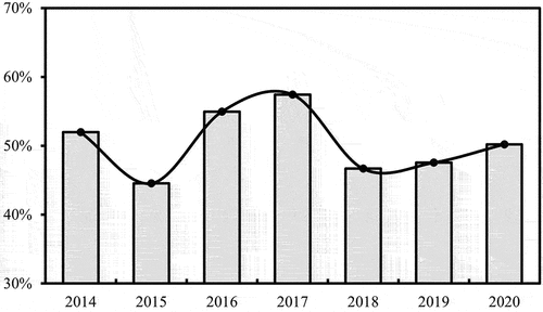
Table 4. OSM data quality at the national scale in China from 2014 to 2020.

Year	Road network length completeness	Relative linear density	Road name attribute completeness	POI name attribute completeness	Road network accuracy	Road network update frequency	POI update frequency	Topological consistency	Directional similarity	T
2014	21.73%	36.39%	20.79%	44.71%	76.37%	47.83%	47.94%	49.41	2.01	51.96%
2015	29.66%	33.54%	20.18%	48.17%	72.38%	35.35%	33.79%	45.55	1.06	44.54%
2016	35.85%	31.38%	20.54%	53.18%	72.44%	29.64%	35.57%	46.89	0.36	54.95%
2017	41.36%	29.16%	20.04%	54.97%	71.88%	29.65%	31.67%	32.37	0.10	57.44%
2018	49.62%	25.43%	19.07%	55.13%	69.39%	23.93%	20.81%	34.54	0.02	46.68%
2019	54.85%	23.58%	18.87%	53.54%	68.75%	21.12%	22.05%	32.87	0.06	47.55%
2020	57.76%	22.87%	18.56%	51.04%	66.90%	29.89%	20.86%	29.03	0.05	50.21%

Figures 7 and 8 show the changes in OSM data quality in China from 2014 to 2020 at the provincial and municipal (with provincial capitals as an example) scales. In general, the OSM data quality in Beijing, Shanghai, Jiangsu, and Guangdong is high, and that in Gansu, Ningxia, Qinghai, and Xinjiang is relatively low. Regarding the temporal trends, for the 31 provinces analyzed at the provincial scale from 2014 to 2020, OSM data quality shows an increasing trend in 22 provinces and a decreasing trend in 9 provinces, with Shaanxi experiencing the most significant decline. At the municipal scale, an upward trend in OSM data quality is observed in the nine provincial capitals, while the trends in the remaining 22 cities exhibit varying degrees of decline.

Figure 7. OSM data quality at the provincial scale in China from 2014 to 2020.

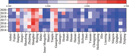
Figure 8. OSM data quality at the municipal scale (taking provincial capitals as an example) in China from 2014 to 2020.

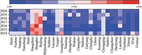
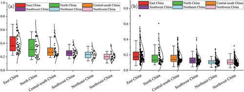
Further analyses (Figures 9 and 10) show that areas with good data quality are mainly concentrated on the southeast side of the Hu Huanyong Line, while areas with poor data quality are concentrated on the northwest side of the Hu Huanyong Line, showing a distribution feature of “dense east and sparse west” that is consistent with economic development and population density. In 1935, the geologist Hu Huanyong proposed the Aihui-Tengchong Line to depict the spatial distribution of the population in China at that time, and the population density was relatively high in areas with good natural conditions, such as those with flat topography, low elevations and adjacent rivers (Cheng, Wang, and Ge 2022). Although the OSM data quality at the municipal scale (Figure 10) does not exhibit a large-scale continuous clustering pattern, it is still evident that there is a patchy distribution in the core areas of the Beijing-Tianjin-Hebei, Yangtze River Delta, Pearl River Delta regions, and around Chongqing. At the provincial and municipal scales, the OSM data quality in the six geographical regions in China decreased in the following order: East China, North China, Central-South China, Southwest China, Northeast China, and Northwest China (Figure 11).

Figure 9. Spatial distribution of OSM data quality at the provincial scale in China in (a) 2014, (b) 2015, (c) 2016, (d) 2017, (e) 2018, (f) 2019, and (g) 2020.

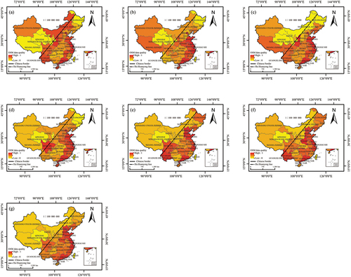
Figure 10. Spatial distribution of OSM data quality at the municipal scale in China in (a) 2014, (b) 2015, (c) 2016, (d) 2017, (e) 2018, (f) 2019, and (g) 2020.

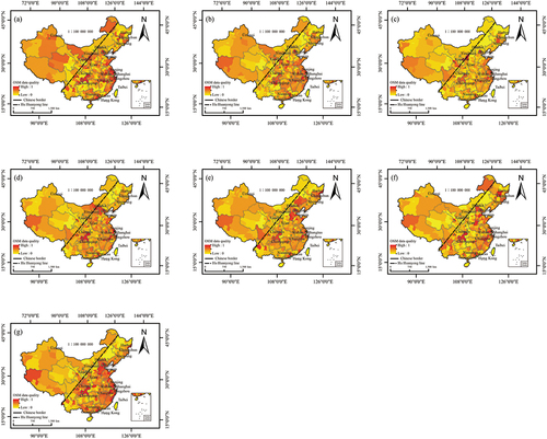
Figure 11. OSM data quality in six geographical regions in China at the (a) provincial scale and (b) municipal scale.

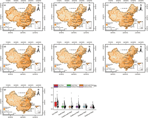
To more comprehensively and accurately reflect the OSM data quality in China, a grid covering all of China was constructed, and each grid cell was 100 × 100 km²; thus, the OSM data quality in China from 2014 to 2020 was represented in the form of grids (Figure 12(a–g)). The OSM data quality still presents the spatial distribution characteristics of high in the east and low in the west at the grid scale. Beijing, Shanghai, Hangzhou and Guangzhou are characterized by high data quality, which is consistent with the data quality evaluation results obtained at the municipal scale. Figure 12(a–g) also reveals an intriguing spatial pattern. Specifically, within the regions characterized by low data quality at the provincial or municipal scale, grid cells that exhibit unexpectedly high data quality at a more local grid scale are observed. This finding indicates that at finer resolutions, there may be localized variations in data quality. Additionally, the trend of OSM data quality of six geographic regions in China at the grid scale is similar to that at the provincial and municipal scales (Figure 12h). This finding verifies the effectiveness of the OSM data quality index system and confirms the feasibility and practicality of the data quality evaluation method proposed in this paper.

Figure 12. Spatial distribution of OSM data quality at the grid scale in China in (a) 2014, (b) 2015, (c) 2016, (d) 2017, (e) 2018, (f) 2019, and (g) 2020. (h) OSM data quality in six geographical regions in China at the grid scale.

At the provincial, municipal, and grid scales, there is a significant difference in OSM data quality between the eastern and western parts of China. These differences may be caused by the economic gap between eastern and western cities. It is well known that the economic capacity of western cities lags far behind that of their eastern counterparts (Shen, Xia, and Li 2022; Zhao et al. 2022), and the poor population in western cities accounts for more than half of the country’s poor population. Therefore, compared with that in the developed cities in the east, the supply of accurate map data in western cities is relatively low.

3.3. Spatial autocorrelation analysis of OSM data quality

3.3.1. Global spatial autocorrelation

Table 5 shows the global Moran’s I values for OSM data quality in China at different spatial scales. Over the period from 2014 to 2020, Moran’s I values are positive and show an increasing trend across provincial, municipal, and grid scales, indicating that the distribution of the OSM data quality in China displays a spatial agglomeration phenomenon and that the spatial agglomeration degree is gradually increasing. Additionally, the analysis reveals certain disparities in the Moran’s I values at different scales, with the highest average Moran’s I values observed at the grid scale. This indicates that the spatial autocorrelation analysis at the grid scale can reflect the internal variations and fine-scale features of OSM data quality in China. The Z-Score and p-Value indicate the spatial correlation level and corresponding significance level in the whole region, respectively. According to the corresponding p-Value for the Moran’s I results, the p-Value in each year at the municipal and grid scales is 0.000, indicating that the 1% significance level test was passed (Z = 1.96). However, at the provincial scale, all the years passed the significance test with a confidence level of 1%, except for 2014, where the p-Value was greater than 0.1, suggesting that the spatial correlation was not significant.

Table 5. Global spatial autocorrelation results based on Moran’s I values from 2014 to 2020.

Spatial scale	Provincial			Municipal			Grid
	$I_{\mathit{Global}}$	Z-Score	P-Value	$I_{\mathit{Global}}$	Z-Score	P-Value	$I_{\mathit{Global}}$	Z-Score	P-Value
2014	0.081	1.503	0.133	0.249	7.697	0.000	0.258	27.060	0.000
2015	0.166	2.607	0.009	0.141	4.834	0.000	0.103	12.724	0.000
2016	0.277	2.949	0.003	0.115	3.891	0.000	0.308	32.944	0.000
2017	0.238	2.525	0.012	0.184	5.816	0.000	0.317	34.897	0.000
2018	0.203	2.178	0.029	0.104	3.346	0.000	0.331	35.054	0.000
2019	0.207	2.209	0.027	0.211	6.578	0.000	0.332	35.682	0.000
2020	0.440	4.325	0.000	0.249	7.782	0.000	0.382	40.206	0.000
Mean	0.230			0.179			0.290

3.3.2. Local spatial autocorrelation

To further explore the spatial characteristics in small areas of the region, a local spatial autocorrelation analysis at the provincial, municipal, and grid scales was performed with equations (24)(24) $I_{\mathit{Local}}=\frac{T_x-\mathit{T}}{S_x^2}\cdot {\sum }_{y=1,y\ne x}^n{W}_{\mathit{xy}}\left(T_y-\mathit{T}\right)$(24) –(25(25) $S_x^2=\frac{{\sum }_{y=1,y\ne x}^n{\left(T_y-\mathit{T}\right)}^2}{\mathit{n}-1}-T^2$(25) ), and a local agglomeration figure was created with ArcGIS software (Figures 13, 14, and Figure 15).

Figure 13. Local spatial autocorrelation distribution of OSM data quality at the provincial scale in (a) 2014, (b) 2015, (c) 2016, (d) 2017, (e) 2018, (f) 2019, and (g) 2020.

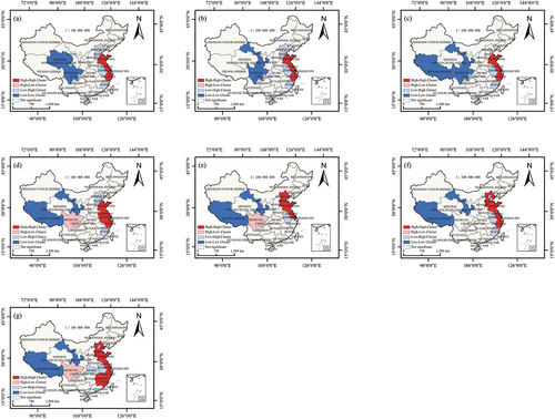
Figure 14. Local spatial autocorrelation distribution of OSM data quality at the municipal scale in (a) 2014, (b) 2015, (c) 2016, (d) 2017, (e) 2018, (f) 2019, and (g) 2020.

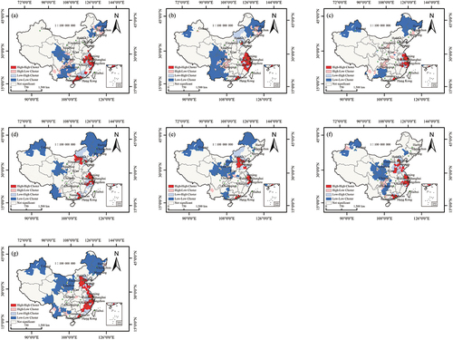
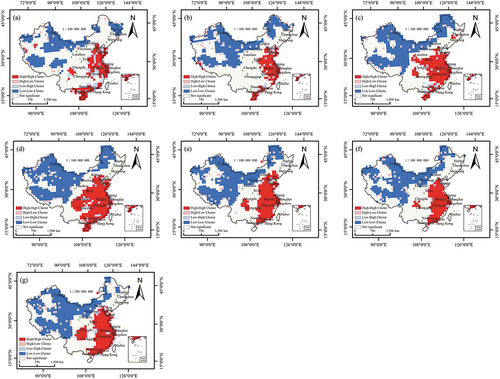
Figure 15. Local spatial autocorrelation distribution of OSM data quality at the grid scale in (a) 2014, (b) 2015, (c) 2016, (d) 2017, (e) 2018, (f) 2019, and (g) 2020.

The local spatial clustering characteristics of the OSM data quality in China are obvious, with mainly high-high (H-H) and low-low (L-L) clusters (Table 6). At the provincial scale, the spatial distribution pattern is relatively stable and significantly differentiated. The provinces in the H-H clusters mainly included Zhejiang, Jiangsu, Shandong and Shanghai, and the scope is expanding continuously. The provinces in the L-L clusters mainly included Gansu and Xizang, and these provinces were generally stable in the H-H and L-L clusters for seven consecutive years, indicating that the local spatial autocorrelation characteristics of most provinces were stable. The provinces in L-H clusters were mainly Anhui and Fujian, and the OSM data quality in surrounding provinces displays high spatial heterogeneity. In addition, Sichuan changed from an L-L cluster to an H-L cluster in 2017, which may be related to changes within that region.

Table 6. Statistics of local spatial autocorrelation for different spatial agglomeration types and scales from 2014 to 2020.

Spatial scale	Spatial agglomeration type	2014	2015	2016	2017	2018	2019	2020
Provincial	HH	4	4	4	5	6	5	8
	HL	0	0	0	1	1	0	1
	LH	3	3	2	2	1	2	2
	LL	2	2	3	2	2	2	2
Municipal	HH	41	42	27	32	31	42	52
	HL	19	17	10	5	8	10	10
	LH	22	15	16	29	17	35	28
	LL	49	70	35	63	52	44	73
Grid	HH	145	120	184	249	189	148	201
	HL	30	46	44	43	42	43	44
	LH	77	49	41	37	27	20	33
	LL	272	348	392	423	402	372	398

Compared with those at the provincial scale, the spatial agglomeration characteristics at the municipal scale are more significant. H-H clusters are mainly distributed in coastal cities in eastern China, such as Shanghai, Guangzhou, and Shenzhen, and the data quality in this region displays a high degree of agglomeration, which is closely related to the data quality in the surrounding areas. As shown in Table 6, from 2014 to 2020, the number of H-H cities changed from 41 to 52, showing an upwards trend. L-L clusters are mainly distributed in Southwest China, Northeast China, and Northwest China, and the number of L-L cities increased from 49 in 2014 to 73 in 2020. For the L-H clusters in East China and North China, the cities with low data quality are surrounded by cities with high data quality. Similarly, for H-L clusters, indicates that the data quality of the city is higher, while that in neighboring cities is comparatively low. Generally, the number of H-L cities shows a downwards trend, while the number of L-H cities shows an upwards trend.

From the grid scale perspective (Figure 15 and Table 6), more regions exhibit positive spatial autocorrelation (H-H and L-L clusters) than negative, and negative spatial correlation types (H-L and L-H) are sporadically distributed. The H-L clusters tend to surround the L-L clusters, whereas the L-H clusters are often distributed around the H-H clusters. In 2014, there were 145 grid cells with H-H clusters and 272 grid cells with L-L clusters, accounting for 27.7% and 51.9%, respectively, of significantly correlated grid cells. By 2020, the number of H-H clusters increased to 201 (29.7%), and the number of L-L clusters increased to 398 (58.9%). Importantly, the local spatial autocorrelation analysis at the grid scale reveals regions with H-H or L-L clusters that were not evident at the municipal scale.

Overall, with variations in spatial scale, the spatiotemporal patterns of OSM data quality in China exhibit relative stability, despite changes in the spatial autocorrelation distribution across multiple administrative levels. Notably, the significant disparities in the spatiotemporal variations in OSM data quality in China are due to the influence of scale dependence and scale effects. Furthermore, large-scale analyses often neglect the intricate spatial patterns present at smaller scales, while small-scale analyses prove more effective in elucidating the spatiotemporal dynamics of regional OSM data quality.

3.4. OSM data quality index and GDP modeling at the provincial and municipal scales

GDP is commonly used to describe regional economic development (Li and Zhang 2017). In this study, OSM data quality index factors were selected as explanatory variables to conduct multiscale GDP modeling to explore the potential of using OSM data quality for economic modeling in China. Provincial and municipal GDP data were obtained from the National Bureau of Statistics of China (http://www.stats.gov.cn/) and the China City Statistical Yearbook (https://www.yearbookchina.com/). The variance inflation factor (VIF) values of all variables at both the provincial and municipal scales are less than 10 (Table 7), indicating no multicollinearity, and all selected variables can be included in the model.

Table 7. Collinearity statistical results.

Spatial scale	Independent variable	VIF	Spatial scale	Independent variable	VIF
Provincial	Road network length completeness	6.247	Municipal	Road network length completeness	1.743
	Relative linear density	5.758		Relative linear density	1.812
	Road name attribute completeness	2.506		Road name attribute completeness	1.206
	POI name attribute completeness	1.579		POI name attribute completeness	1.179
	Road network accuracy	1.925		Road network accuracy	1.168
	Road network update frequency	1.592		Road network update frequency	1.291
	POI update frequency	1.369		POI update frequency	1.283
	Topological consistency	1.369		Topological consistency	1.081
	Directional similarity	1.771		Directional similarity	1.074

Comparing the performance of the GWR and GTWR models by using adjusted-R², residual sum of squares (RSS), and AICc (Table 8). The GTWR model showed notable improvements in adjusted R² values (0.86 at the provincial scale and 0.88 at the municipal scale) compared to the GWR model. And it also produced lower AICc and RSS values, indicating higher explanatory power. Additionally, R² values increased with decreasing spatial scale (provincial to municipal), suggesting that the correlations among data increased with decreasing spatial scale.

Table 8. OSM data quality and GDP modeling results at the provincial and municipal scales in China.

Spatial scale	Model	R^2	Adjusted-R^2	AICc	RSS
Provincial	GWR	0.8475	0.8106	−85.9606	5.9436
	GTWR	0.8953	0.8585	−130.2082	4.0824
Municipal	GWR	0.8775	0.8518	−890.0355	63.2534
	GTWR	0.9063	0.8753	−1066.2704	48.3905

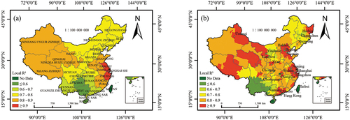
The local R² of the provincial- and municipal-scale GTWR models (Figure 16) were visualized to explore the spatial heterogeneity of relationships among the data. Notably, the local R² vary across regions, but their trends at different scales remain consistent. The proportion of local R² greater than 0.8 at the provincial scale is 38.7%, while at the municipal scale, this proportion increases to 65.0%, with most of these areas distributed in the economically underdeveloped areas in Northwest China and the economically developed areas in East China. The results of the GTWR model not only further verify the advantages of using the OSM data quality index system in provincial- and municipal-scale GDP modeling in China but also indicate that the OSM data quality index approach has certain potential in the economic modeling of economically underdeveloped regions.

Figure 16. Local R² spatial distribution of the GTWR model at the (a) provincial scale and (b) municipal scale.

Figure 17 shows the spatial distribution of individual factor regression coefficients for the GTWR model at the municipal scale. The average regression coefficients for each variable are as follows: 4.06, 1.40, 0.17, 0.23, 0.71, 1.68, 1.10, 1.33, and −0.05, respectively. Data quality index factors affecting the GDP vary with spatial location, with most index factors showing a positive spatial correlation with GDP, except for directional similarity. These results demonstrate the spatially nonstationarity relationship between GDP and OSM data quality index factors.

Figure 17. Spatial distribution of regression coefficients for the GTWR model at the municipal scale.

3.5. GDP simulation at the grid scale

To explore whether the OSM data quality index system at the grid-scale can reflect regional economic development, the indicator factors in 2020 were selected as input variables. The correlation between the nighttime light (NTL) data (https://ngdc.noaa.gov/) and GDP data is significant (Ma et al. 2014); as a result, it is possible to utilize the NTL data in conjunction with the ordinary least squares (OLS) model to allocate GDP values to each pixel of the NTL dataset and generate the grid-scale GDP (Dai, Hu, and Zhao 2017; Zhao et al. 2023). The specific steps are as follows: (1) the total nighttime light (TNL) intensity at the municipal scale is computed as the cumulative sum of all pixels within the respective administrative region; (2) a regression model of TNL and GDP is established, and the regression coefficient is calculated; (3) the regression coefficient and NTL data are used to simulate grid-scale GDP ($\mathit{GD}{P}_G$); and (4) the corrected grid-scale GDP is obtained by correcting the predicted GDP based on the municipal GDP statistics ($\mathit{GD}{P}_M$). The equation is $\mathit{GD}{P}_G\times \mathit{GD}{P}_M/\mathit{GD}{P}_T$, where $\mathit{GD}{P}_T$ is the sum of the predicted GDP values in the region. All GDP data were log transformed as the dependent variable of the final model. Four machine learning models, SVM, RF, XGBoost and CatBoost, were used to simulate GDP at the grid scale. RStudio software was used to randomly divide the data into a training set and a test set at a ratio of 7:3.

Table 9 presents the training and testing results of the four machine learning models for predicting grid cell GDP using OSM data quality. The R² values for all model test sets exceed 0.60. Notably, the CatBoost model yields the highest simulation accuracy, achieving R², RMSE, and MAE values of 0.82, 0.56, and 0.40, respectively. This indicates its superior capability in capturing the underlying relationships between OSM data quality and grid GDP. In conclusion, Table 9 provides evidence of the predictive power of the machine learning models in the context of grid-cell GDP prediction using OSM data quality, and the superior performance and accuracy of the CatBoost model suggest that it can be an effective tool for both researchers and practitioners to predict regional economic development at the grid-cell resolution.

Table 9. Comparison of the accuracy of the GDP simulation results of different machine learning models.

Machine learning model	Dataset	R^2	RMSE	MAE
SVM	Training set	0.5926	0.9097	0.5561
	Test set	0.6286	0.7512	0.5030
RF	Training set	0.7902	0.7717	0.4521
	Test set	0.7472	0.6230	0.7902
XGBoost	Training set	0.9314	0.5770	0.2429
	Test set	0.7716	0.6278	0.4167
CatBoost	Training set	0.8768	0.6696	0.3226
	Test set	0.8152	0.5582	0.3961

4. Discussion

Spatial data quality evaluation is the main basis for assessing data availability. Previous research has demonstrated a concentration of richer OSM data in the developed cities of the eastern regions, while areas of lower data quality predominantly exist in the western and southwestern regions of China (Su et al. 2017; Zheng and Zheng 2014). However, these studies only considered two indicators, completeness, and position accuracy. On the one hand, these indicators are relatively single, and on the other hand, there is a lack of overall comprehensive evaluation. In this study, we developed a unified measure for OSM data quality evaluation index system. Combined with the EWM-TOPSIS model, the OSM data quality in China was evaluated comprehensively for the first time. In terms of weighting methods, traditional weighting methods are often calculated according to experience or artificially set weights, ignoring the relevance and importance of each indicator. The EWM can better reflect the importance and difference of each indicator (Zhou et al. 2022). Consequently, this research employed the EWM to compute indicator weights across different scales, along with an analysis of the significance of quality dimensions within these scales. The findings indicated fluctuations in the weights of different quality dimensions. On a larger scale, ensuring temporal accuracy of data emerges as critically important. Conversely, at a finer scale, precise geographical positioning may wield greater influence on data quality, revealing the intricacy of data quality dimensions across diverse spatial scales. By combining the computed indicator weights with the TOPSIS comprehensive evaluation model, more precise assessments of data quality can be obtained (Wang et al. 2022). The experimental results show the feasibility and practicability of the EWM-TOPSIS model, which provides empirical evidence and a reliable data quality assessment method that facilitates various applications, not only in industry but also in research and within the OSM community itself based on VGI data sources. In addition, the results of the study (Figures 9–12) also can help the volunteers understand where OSM data quality needed to be improved.

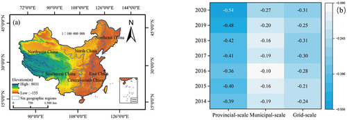
By employing a unified metric, a more comprehensive understanding of OSM data quality can be achieved, enabling easy investigations and visualizations of data quality levels at different scales. The results of the OSM data quality evaluation at the provincial and municipal scales show that areas with high data quality are more concentrated on the southeast side of the Hu Huanyong Line, while areas with low data quality are distributed on the northwest side of the Hu Huanyong Line (Figures 9 and 10), further confirming the close relationship between OSM data quality and population, which supports the conclusions of previous studies that areas with high population density have more VGI contributions (Borkowska and Pokonieczny 2022; Jokar Arsanjani et al. 2013; Minaei 2020; Neis, Zielstra, and Zipf 2013). In addition, we found that the OSM data quality of six geographic regions in China, East China, North China, Central-South China, Southwest China, Northeast China, and Northwest China, decreases. East China, North China, and Central-South China are economic development centers in China. These regions have rapid urbanization, high population density, complete traffic construction and relatively concentrated social resources, so the collection and update of OSM data are relatively timely and comprehensive. However, Southwest China, Northeast China, and Northwest China have almost opposite trends in terms of the economy and population density, so there is a lag in the corresponding OSM data updates, and the data quality is relatively low. Another important factor leading to the low data quality in Northwest China and Southwest China is the geographical environment. The topography of Northwest China and Southwest China is complex (Figure 18a) and includes mountain, desert, and basin geomorphic types. For a better explanation, we explored the relationship between OSM data quality and the digital elevation model (DEM) at different spatial scales from 2014 to 2017. The results show that OSM data quality and elevation at different spatial scales have obvious negative correlations (Figure 18b). Notably, this correlation is strongest at the provincial scale and gradually increases over time, reaching −0.54 in 2020, which further indicates that the topography may influence OSM data quality to a certain extent.

Figure 18. (a) DEM of six geographical regions in China. (b) Correlation between OSM data quality and DEM at different spatial scales.

Another innovation of this paper is the use of OSM data quality indicators as a proxy to estimate regional economic development. Previous studies used the geographic data in the OSM database (e.g. OSM road network density and POI) as a proxy to reflect regional economic development (Feldmeyer et al. 2020; Liu et al. 2020). However, due to did not evaluate the quality of these data, the results may lead to certain errors. In contrast, by using OSM data quality indicators to simulate the GDP, multiple aspects of urban economic development, such as the completeness of road networks and infrastructure and the frequency of data updates, can be more comprehensively considered, thereby improving the accuracy of estimates. The results show that that the application of the unified measure proposed in this research enables accurate predictions of economic development across various spatial scales. This provides an effective reference indicator for accurately assessing regional economic development in data-scarce and underdeveloped regions.

This study has several limitations. First, due to the limited accessibility of high-quality datasets, it is impossible to establish a one-to-one correspondence between OSM road or POI tags and true names, leading to the incomplete evaluation of attribute accuracy. Second, in terms of the calculation of topological consistency, this study only addresses the polyline topology. Topological errors of geospatial data include many aspects, such as polyline and polygon, point and polyline, which need further analysis. Third, OSM data include not only roads and POIs but also other element types, such as lakes and buildings. In this paper, only road and POI data were systematically evaluated. In the next step, all element types should be considered to evaluate OSM data in a more comprehensive way.

As OSM data continues to grow and update, gradually establishing itself as a significant online mapping platform (Anderson, Sarkar, and Palen 2019; Herfort et al. 2021), the future evaluation of OSM data quality remains a crucial research focus (Tzavella, Skopeliti, and Fekete 2022). Our study developed a comprehensive OSM data quality assessment indicator system, comprising diverse key dimensions of quality to ensure an all-encompassing evaluation of data quality. This framework is poised to play a vital role in guiding the management and maintenance of OSM data quality in the future, aiding users and researchers in better understanding and utilizing data quality information. Furthermore, our study employed the EWM-TOPSIS model to conduct an assessment of OSM data quality in China. The application of this model provides a feasible and effective approach for comprehensively evaluating OSM data quality across diverse regions and countries in future research. It offers visualizations that readily identify regions with lower data quality, providing a valuable foundation for optimizing data allocation strategies. By promptly identifying and addressing data quality issues, we could significantly enhance the reliability and accuracy of data applications, thereby contributing to the advancement and growth of the OSM community. Additionally, the comprehensive assessment results obtained from the EWM-TOPSIS model could offer clear improvement directions for volunteers in improving the OSM data quality. Understanding the weights of different quality dimensions allows volunteers to make targeted improvements in data collection and maintenance strategies, thus elevating overall data quality. This fosters a continuous process of improvement, enabling future OSM data can play a more significant and impactful role in diverse application domains.

5. Conclusions

In this paper, an OSM data quality evaluation index system in China is constructed considering the completeness, attribute accuracy, position accuracy, temporal accuracy, and logical consistency of OSM data. Using the China Statistical Yearbook and Baidu Maps as reference data, the EWM-TOPSIS model is used to analyze the quality of Chinese OSM data from 2014 to 2020 in detail. The GTWR model is used to explore the potential of OSM data quality indicators in economic modeling at the provincial and municipal scales in China. Finally, a variety of machine learning algorithms are used for grid-scale GDP simulation. The main conclusions are as follows.

1. The weights of OSM data quality indicators exhibit significant variations across different spatial scales. “Temporal accuracy” holds considerable importance at the national, provincial, and municipal scales, with its weight increasing as the spatial scale decreases, reaching approximately 47% at the municipal scale. However, at the finer grid scale, “position accuracy” has the most significant impact on data quality.

2. From 2014 to 2020, the OSM data quality at the national scale displayed a trend of first increasing, then decreasing and then gradually stabilizing, with the best data quality in 2017. The OSM data quality at different spatial scales displayed a spatiotemporal distribution of high in the east and low in the west, which is influenced by population and geographical environment.

3. The OSM data quality at different scales in China displays a significant positive correlation in space, with notable spatial clustering, and the degree of spatial autocorrelation has increased over time. In addition, the quality of Chinese OSM data exhibits obvious local spatial autocorrelation characteristics, which are dominated by H-H and L-L clusters. From 2014 to 2020, the local spatial autocorrelation characteristics at the provincial scale were relatively stable, while the H-H clustering and the L-L clustering at the municipal and grid scales showed an upward trend.

4. The GTWR model performs well in predicting and revealing the correlation characteristics between the provincial- and municipal-scale GDP and OSM data quality indicators in China from the perspectives of time and space. The adjusted R² was 0.86 at the provincial scale and 0.88 at the municipal scale, and the correlations among the data increased with decreasing spatial scale (provincial to municipal scale). The 38.7% of regions at the provincial scale and 65.0% of regions at the municipal scale with local R² greater than 0.8 were mainly distributed in the economically underdeveloped areas in Northwest China and the economically developed areas in East China.

5. The grid-scale GDP was well simulated by using the OSM data quality index combined with machine learning models. The simulation accuracy of the four models was ranked in descending order as follows: CatBoost > XGBoost > RF > SVM. The CatBoost model displayed the best performance, with R², RMSE and MAE values of 0.82, 0.56, and 0.40, respectively, suggesting that the CatBoost model has great potential for use in simulating GDP at the grid scale.

Disclosure statement

No potential conflict of interest was reported by the author(s).

Data availability statement

The OpenStreetMap data were sourced from the official website of OSM (https://www.openstreetmap.org/). Reference road vector data were obtained from Baidu Maps (https://map.baidu.com/). The vector boundary of the research area was obtained from the Chinese Resource and Environment Science and Data Center (https://www.resdc.cn/). The actual road mileage data, Provincial and municipal GDP were obtained from the National Bureau of Statistics of China (http://www.stats.gov.cn/) and the China City Statistical Yearbook (https://www.yearbookchina.com/).

Additional information

Funding

This work is supported by The National Natural Science Foundation of China [grant number 41461035], Xinjiang “Tianshan Cedar” project [grant number 2020XS04], and Excellent Doctoral Innovation Project of Xinjiang University [XJU2024BS076].

Notes on contributors

Chuqiao Han

Chuqiao Han is currently a Ph.D. candidate at Xinjiang University. He focuses on research in spatiotemporal big data and geographic information system modeling.

Binbin Lu

Binbin Lu currently holds the position of associate professor at Wuhan University. His research focuses on geocomputation, spatial statistics, geographically weighted (GW) modeling, open-source GIS, R coding, and spatio-temporal big data analysis.

Jianghua Zheng

Jianghua Zheng is a Professor of the College of Geographical and Remote Sensing Science at Xinjiang University. His research interests include vegetation and environmental remote sensing, monitoring and safety assessment of forest and grassland ecosystems, as well as research in remote sensing and geographic information systems applications.

Danlin Yu

Danlin Yu is a professor at Montclair State University. His research interests are geographic information analysis, cartographical design and presentation, statistical analysis, urban and regional planning, and system dynamic modeling.

Shudan Zheng

Shudan Zheng received his Master’s degree from Xinjiang University and is currently employed as an engineer at Lantmäteriet. Her research focus is on geographic information system development and applications.

References

- Anderson, J., D. Sarkar, and L. Palen. 2019. “Corporate Editors in the Evolving Landscape of OpenStreetmap.” ISPRS International Journal of Geo-Information 8 (5): 232. https://doi.org/10.3390/ijgi8050232.
- Barrington-Leigh, C., A. Millard-Ball, and M. Ali. 2017. “The World’s User-Generated Road Map is More Than 80% Complete.” PLOS ONE 12 (8): e0180698. https://doi.org/10.1371/journal.pone.0180698.
- Barrington-Leigh, C., and A. Millard-Ball. 2020. “Global Trends Toward Urban Street-Network Sprawl.” Proceedings of the National Academy of Sciences 117 (4): 1941–1950. https://doi.org/10.1073/pnas.1905232116.
- Barron, C., P. Neis, and A. Zipf. 2014. “A Comprehensive Framework for Intrinsic OpenStreetmap Quality Analysis.” Transactions in GIS 18 (6): 877–895. https://doi.org/10.1111/tgis.12073.
- Blower, J. D., J. Masó, D. Díaz, C. J. Roberts, G. H. Griffiths, J. P. Lewis, X. Yang, and X. Pons. 2015. “Communicating Thematic Data Quality with Web Map Services.” ISPRS International Journal of Geo-Information 4 (4): 1965–1981. https://doi.org/10.3390/ijgi4041965.
- Borkowska, S., E. Bielecka, and K. Pokonieczny. 2023. “Comparison of Land Cover Categorical Data Stored in OSM and Authoritative Topographic Data.” Applied Sciences 13 (13): 7525. https://doi.org/10.3390/app13137525.
- Borkowska, S., and K. Pokonieczny. 2022. “Analysis of OpenStreetmap Data Quality for Selected Counties in Poland in Terms of Sustainable Development.” Sustainability 14 (7): 3728. https://doi.org/10.3390/su14073728.
- Bray, M., and D. Han. 2004. “Identification of Support Vector Machines for Runoff Modelling.” Journal of Hydroinformatics 6 (4): 265–280. https://doi.org/10.2166/hydro.2004.0020.
- Breiman, L. 2001. “Random Forests.” Machine Learning 45 (1): 5–32. https://doi.org/10.1023/A:1010933404324.
- Bright, J., S. De Sabbata, S. Lee, B. Ganesh, and D. K. Humphreys. 2018. “OpenStreetmap Data for Alcohol Research: Reliability Assessment and Quality Indicators.” Health & Place 50 (3): 130–136. https://doi.org/10.1016/j.healthplace.2018.01.009.
- Brodeur, J. 2001. “Standardization in Geomatics: In Canada and in Iso/Tc 211.” Geomatica 55 (1): 91–106. NRC Research Press. https://doi.org/10.5623/geomat-2001-0011.
- Brodeur, J., S. Coetzee, D. Danko, S. Garcia, and J. Hjelmager. 2019. “Geographic Information Metadata—An Outlook from the International Standardization Perspective.” ISPRS International Journal of Geo-Information 8 (6): 280. https://doi.org/10.3390/ijgi8060280.
- Chaves Carniel, A. 2023. “Defining and Designing Spatial Queries: The Role of Spatial Relationships.” Geo-Spatial Information Science: 1–25. https://doi.org/10.1080/10095020.2022.2163924.
- Chen, T., and C. Guestrin. 2016. “XGBoost: A Scalable Tree Boosting System.” Paper presented at the 22nd ACM SIGKDD International Conference on Knowledge Discovery and Data Mining, 785–794. New York, August. https://doi.org/10.1145/2939672.2939785.
- Cheng, Z., J. Wang, and Y. Ge. 2022. “Mapping Monthly Population Distribution and Variation at 1-Km Resolution Across China.” International Journal of Geographical Information Science 36 (6): 1166–1184. https://doi.org/10.1080/13658816.2020.1854767.
- Dai, Z., Y. Hu, and G. Zhao. 2017. “The Suitability of Different Nighttime Light Data for GDP Estimation at Different Spatial Scales and Regional Levels.” Sustainability 9 (2): 305. https://doi.org/10.3390/su9020305.
- Degrossi, L. C., J. P. de Albuquerque, R. dos Santos Rocha, and A. Zipf. 2018. “A Taxonomy of Quality Assessment Methods for Volunteered and Crowdsourced Geographic Information.” Transactions in GIS 22 (2): 542–560. https://doi.org/10.1111/tgis.12329.
- Despotovic, M., V. Nedic, D. Despotovic, and S. Cvetanovic. 2015. “Review and Statistical Analysis of Different Global Solar Radiation Sunshine Models.” Renewable and Sustainable Energy Reviews 52 (12): 1869–1880. https://doi.org/10.1016/j.rser.2015.08.035.
- Elias, E. N. N., V. de Oliveira Fernandes, M. J. Alixandrini Junior, and M. A. R. Schmidt. 2020. “The Quality of OpenStreetmap in a Large Metropolis in Northeast Brazil: Preliminary Assessment of Geospatial Data for Road Axes.” Boletim de Ciências Geodésicas 26 (3): e2020012–e2020012. https://doi.org/10.1590/s1982-21702020000300012.
- Fan, H., A. Zipf, Q. Fu, and P. Neis. 2014. “Quality Assessment for Building Footprints Data on OpenStreetmap.” International Journal of Geographical Information Science 28 (4): 700–719. https://doi.org/10.1080/13658816.2013.867495.
- Feldmeyer, D., C. Meisch, H. Sauter, and J. Birkmann. 2020. “Using OpenStreetmap Data and Machine Learning to Generate Socio-Economic Indicators.” ISPRS International Journal of Geo-Information 9 (9): 498. https://doi.org/10.3390/ijgi9090498.
- Forghani, M., and M. Reza Delavar. 2014. “A Quality Study of the OpenStreetmap Dataset for Tehran.” ISPRS International Journal of Geo-Information 3 (2): 750–763. https://doi.org/10.3390/ijgi3020750.
- Gao, C., L. Xu, and W. Li. 2021. “Research on Visualization Method of Congestion Pattern in Urban Transportation Hub.” Paper presented at 2021 2nd International Conference on Artificial Intelligence and Information Systems, New York, May 1–6. https://doi.org/10.1145/3469213.3470239.
- Girres, J.-F., and G. Touya. 2010. “Quality Assessment of the French OpenStreetmap Dataset.” Transactions in GIS 14 (4): 435–459. https://doi.org/10.1111/j.1467-9671.2010.01203.x.
- Goldblatt, R., N. Jones, and J. Mannix. 2020. “Assessing OpenStreetmap Completeness for Management of Natural Disaster by Means of Remote Sensing: A Case Study of Three Small Island States (Haiti, Dominica and St. Lucia).” Remote Sensing 12 (1): 118. https://doi.org/10.3390/rs12010118.
- Goodchild, M. F. 2007. “Citizens as Sensors: The World of Volunteered Geography.” Geo Journal 69 (4): 211–221. https://doi.org/10.1007/s10708-007-9111-y.
- Goodchild, M. F., and L. Li. 2012. “Assuring the Quality of Volunteered Geographic Information.” Spatial Statistics 1 (5): 110–120. https://doi.org/10.1016/j.spasta.2012.03.002.
- Griffith, D. A., and G. Arbia. 2010. “Detecting Negative Spatial Autocorrelation in Georeferenced Random Variables.” International Journal of Geographical Information Science 24 (3): 417–437. https://doi.org/10.1080/13658810902832591.
- Hadimlioglu, I. A., and S. A. King. 2019. “City Maker: Reconstruction of Cities from OpenStreetmap Data for Environmental Visualization and Simulations.” ISPRS International Journal of Geo-Information 8 (7): 298. https://doi.org/10.3390/ijgi8070298.
- Haklay, M., and P. Weber. 2008. “OpenStreetmap: User-Generated Street Maps.” IEEE Pervasive Computing 7 (4): 12–18. https://doi.org/10.1109/MPRV.2008.80.
- Han, C., J. Zheng, J. Guan, D. Yu, and B. Lu. 2022. “Evaluating and Simulating Resource and Environmental Carrying Capacity in Arid and Semiarid Regions: A Case Study of Xinjiang, China.” Journal of Cleaner Production 338 (3): 130646. https://doi.org/10.1016/j.jclepro.2022.130646.
- Hashemi, P., and R. A. Abbaspour. 2015. “Assessment of Logical Consistency in OpenStreetmap Based on the Spatial Similarity Concept.” In OpenStreetmap in GIScience: Experiences, Research, and Applications, edited by J. J. Arsanjani, A. Zipf, P. Mooney, and M. Helbich, 19–36. Berlin: Springer. https://doi.org/10.1007/978-3-319-14280-7_2.
- Hecht, R., C. Kunze, and S. Hahmann. 2013. “Measuring Completeness of Building Footprints in OpenStreetmap Over Space and Time.” ISPRS International Journal of Geo-Information 2 (4): 1066–1091. https://doi.org/10.3390/ijgi2041066.
- Herfort, B., S. Lautenbach, J. P. de Albuquerque, J. Anderson, and A. Zipf. 2021. “The Evolution of Humanitarian Mapping within the OpenStreetmap Community.” Scientific Reports 11 (1): 3037. https://doi.org/10.1038/s41598-021-82404-z.
- Huang, B., B. Wu, and M. Barry. 2010. “Geographically and Temporally Weighted Regression for Modeling Spatio-Temporal Variation in House Prices.” International Journal of Geographical Information Science 24 (3): 383–401. https://doi.org/10.1080/13658810802672469.
- Huang, G., L. Wu, X. Ma, W. Zhang, J. Fan, X. Yu, W. Zeng, and H. Zhou. 2019. “Evaluation of CatBoost Method for Prediction of Reference Evapotranspiration in Humid Regions.” Journal of Hydrology 574 (7): 1029–1041. https://doi.org/10.1016/j.jhydrol.2019.04.085.
- Husen, S. N. R. M., N. H. Idris, and M. H. I. Ishak. 2018. “The Quality of OpenStreetmap in Malaysia: A Preliminary Assessment.” International Archives of the Photogrammetry, Remote Sensing and Spatial Information Sciences XLII-4 (W9): 291–298. https://doi.org/10.5194/isprs-archives-XLII-4-W9-291-2018.
- Jacobs, K. T., and S. W. Mitchell. 2020. “OpenStreetmap Quality Assessment Using Unsupervised Machine Learning Methods.” Transactions in GIS 24 (5): 1280–1298. https://doi.org/10.1111/tgis.12680.
- Jahanshahloo, G. R., F. Hosseinzadeh Lotfi, and M. Izadikhah. 2006. “Extension of the TOPSIS Method for Decision-Making Problems with Fuzzy Data.” Applied Mathematics and Computation 181 (2): 1544–1551. https://doi.org/10.1016/j.amc.2006.02.057.
- Jokar Arsanjani, J., Z. Alexander, M. Peter, and M. Helbich. 2015. “An Introduction to OpenStreetmap in Geographic Information Science: Experiences, Research, and Applications.” In OpenStreetmap in GIScience: Experiences, Research, and Applications, edited by J. J. Arsanjani, A. Zipf, P. Mooney, and M. Helbich, 1–15. Berlin: Springer. https://doi.org/10.1007/978-3-319-14280-7_1.
- Jokar Arsanjani, J., M. Helbich, M. Bakillah, J. Hagenauer, and A. Zipf. 2013. “Toward Mapping Land-Use Patterns from Volunteered Geographic Information.” International Journal of Geographical Information Science 27 (12): 2264–2278. https://doi.org/10.1080/13658816.2013.800871.
- Jokar Arsanjani, J., M. Peter, Z. Alexander, and S. Anne. 2015. “Quality Assessment of the Contributed Land Use Information from OpenStreetmap versus Authoritative Datasets.” In OpenStreetmap in GIScience: Experiences, Research, and Applications, edited by J. J. Arsanjani, A. Zipf, P. Mooney, and M. Helbich, 37–58. Berlin: Springer. https://doi.org/10.1007/978-3-319-14280-7_3.
- Klonner, C., M. Hartmann, R. Dischl, L. Djami, L. Anderson, M. Raifer, F. Lima-Silva, L. C. Degrossi, A. Zipf, and J. P. de Albuquerque. 2021. “The Sketch Map Tool Facilitates the Assessment of OpenStreetmap Data for Participatory Mapping.” ISPRS International Journal of Geo-Information 10 (3): 130. https://doi.org/10.3390/ijgi10030130.
- Li, C., K. Wu, and X. Gao. 2020. “Manufacturing Industry Agglomeration and Spatial Clustering: Evidence from Hebei Province, China.” Environment, Development and Sustainability 22 (4): 2941–2965. https://doi.org/10.1007/s10668-019-00328-1.
- Li, C., and X. Zhang. 2017. “Renminbi Internationalization in the New Normal: Progress, Determinants and Policy Discussions.” China & World Economy 25 (2): 22–44. https://doi.org/10.1111/cwe.12192.
- Li, J., H. Qin, J. Wang, and J. Li. 2022. “OpenStreetmap-Based Autonomous Navigation for the Four Wheel-Legged Robot via 3D-Lidar and CCD Camera.” IEEE Transactions on Industrial Electronics 69 (3): 2708–2717. https://doi.org/10.1109/TIE.2021.3070508.
- Lin, S.-S., S.-L. Shen, A. Zhou, and Y.-S. Xu. 2020. “Approach Based on TOPSIS and Monte Carlo Simulation Methods to Evaluate Lake Eutrophication Levels.” Water Research 187 (12): 116437. https://doi.org/10.1016/j.watres.2020.116437.
- Liu, B., Y. Shi, D.-J. Li, Y.-D. Wang, G. Fernandez, and M.-H. Tsou. 2020. “An Economic Development Evaluation Based on the OpenStreetmap Road Network Density: The Case Study of 85 Cities in China.” ISPRS International Journal of Geo-Information 9 (9): 517. https://doi.org/10.3390/ijgi9090517.
- Lu, B., Y. Hu, D. Murakami, C. Brunsdon, A. Comber, M. Charlton, and P. Harris. 2022. “High-Performance Solutions of Geographically Weighted Regression in R.” Geo-Spatial Information Science 25 (4): 536–549. https://doi.org/10.1080/10095020.2022.2064244.
- Luo, N., T. Wan, H. Hao, and Q. Lu. 2019. “Fusing High-Spatial-Resolution Remotely Sensed Imagery and OpenStreetmap Data for Land Cover Classification Over Urban Areas.” Remote Sensing 11 (1): 88. https://doi.org/10.3390/rs11010088.
- Ma, T., Y. Zhou, Y. Wang, C. Zhou, S. Haynie, and T. Xu. 2014. “Diverse Relationships Between Suomi-NPP VIIRS Night-Time Light and Multi-Scale Socioeconomic Activity.” Remote Sensing Letters 5 (7): 652–661. https://doi.org/10.1080/2150704X.2014.953263.
- Medeiros, G., and M. Holanda. 2019. “Solutions for Data Quality in GIS and VGI: A Systematic Literature Review.” In New Knowledge in Information Systems and Technologies, 645–654. Berlin: Springer. https://doi.org/10.1007/978-3-030-16181-1_61.
- Meng, Y., F. Ni, Y. Deng, J. Feng, Z. Sheng, and C. Luo. 2018. “Ecological Risk Assessment of Water Resources in Ya’an City Based on EWM-TOPSIS.” Ekoloji 27 (106): 1765–1774.
- Minaei, M. 2020. “Evolution, Density and Completeness of OpenStreetmap Road Networks in Developing Countries: The Case of Iran.” Applied Geography 119 (6): 102246. https://doi.org/10.1016/j.apgeog.2020.102246.
- Minghini, M., and F. Frassinelli. 2019. “OpenStreetmap History for Intrinsic Quality Assessment: Is OSM Up-To-Date?” Open Geospatial Data, Software and Standards 4 (1): 9. https://doi.org/10.1186/s40965-019-0067-x.
- Mooney, P., and L. Morgan. 2015. “How Much Do We Know About the Contributors to Volunteered Geographic Information and Citizen Science Projects?” ISPRS Annals of the Photogrammetry, Remote Sensing & Spatial Information Sciences II-3 (W5): 339–343. https://doi.org/10.5194/isprsannals-II-3-W5-339-2015.
- Muttaqien, B. I., F. O. Ostermann, and R. L. G. Lemmens. 2018. “Modeling Aggregated Expertise of User Contributions to Assess the Credibility of OpenStreetmap Features.” Transactions in GIS 22 (3): 823–841. https://doi.org/10.1111/tgis.12454.
- Nasiri, A., R. Ali Abbaspour, A. Chehreghan, and J. Jokar Arsanjani. 2018. “Improving the Quality of Citizen Contributed Geodata Through Their Historical Contributions: The Case of the Road Network in OpenStreetmap.” ISPRS International Journal of Geo-Information 7 (7): 253. https://doi.org/10.3390/ijgi7070253.
- Neis, P., and D. Zielstra. 2014. “Recent Developments and Future Trends in Volunteered Geographic Information Research: The Case of OpenStreetmap.” Future Internet 6 (1): 76–106. https://doi.org/10.3390/fi6010076.
- Neis, P., D. Zielstra, and A. Zipf. 2012. “The Street Network Evolution of Crowdsourced Maps: OpenStreetmap in Germany 2007–2011.” Future Internet 4 (1): 1–21. https://doi.org/10.3390/fi4010001.
- Neis, P., D. Zielstra, and A. Zipf. 2013. “Comparison of Volunteered Geographic Information Data Contributions and Community Development for Selected World Regions.” Future Internet 5 (2): 282–300. https://doi.org/10.3390/fi5020282.
- Novack, T., L. Vorbeck, and A. Zipf. 2022. “An Investigation of the Temporality of OpenStreetmap Data Contribution Activities.” Geo-Spatial Information Science 27 (2): 259–275. https://doi.org/10.1080/10095020.2022.2124127.
- Ord, J. K., and A. Getis. 1995. “Local Spatial Autocorrelation Statistics: Distributional Issues and an Application.” Geographical Analysis 27 (4): 286–306. https://doi.org/10.1111/j.1538-4632.1995.tb00912.x.
- Prokhorenkova, L., G. Gusev, A. Vorobev, A. Veronika Dorogush, and A. Gulin. 2018. “CatBoost: Unbiased Boosting with Categorical Features.” Advances in Neural Information Processing Systems: 31. https://doi.org/10.48550/arXiv.1706.09516.
- Qiu, M., Q. Zuo, Q. Wu, Z. Yang, and J. Zhang. 2022. “Water Ecological Security Assessment and Spatial Autocorrelation Analysis of Prefectural Regions Involved in the Yellow River Basin.” Scientific Reports 12 (1): 1–15. https://doi.org/10.1038/s41598-022-07656-9.
- Rafi, S., W. Yu, M. Azeem Akbar, A. Alsanad, and A. Gumaei. 2020. “Multicriteria Based Decision Making of DevOps Data Quality Assessment Challenges Using Fuzzy TOPSIS.” IEEE Access 8:46958–46980. https://doi.org/10.1109/ACCESS.2020.2976803.
- Saaty, T. L. 2013. “The Modern Science of Multicriteria Decision Making and its Practical Applications: The AHP/ANP Approach.” Operations Research 61 (5): 1101–1118. https://doi.org/10.1287/opre.2013.1197.
- Schellekens, J., R. J. Brolsma, R. J. Dahm, G. V. Donchyts, and H. C. Winsemius. 2014. “Rapid Setup of Hydrological and Hydraulic Models Using OpenStreetmap and the SRTM Derived Digital Elevation Model.” Environmental Modelling & Software 61 (11): 98–105. https://doi.org/10.1016/j.envsoft.2014.07.006.
- See, L., P. Mooney, G. Foody, L. Bastin, A. Comber, J. Estima, S. Fritz, et al. 2016. “Crowdsourcing, Citizen Science or Volunteered Geographic Information? The Current State of Crowdsourced Geographic Information.” ISPRS International Journal of Geo-Information 5 (5): 55. https://doi.org/10.3390/ijgi5050055.
- Senaratne, H., A. Mobasheri, A. Loai Ali, C. Capineri, and M. (. Haklay. 2017. “A Review of Volunteered Geographic Information Quality Assessment Methods.” International Journal of Geographical Information Science 31 (1): 139–167. https://doi.org/10.1080/13658816.2016.1189556.
- Shabani, M., Z. Masoumi, and A. Rezaei. 2022. “Assessment of Groundwater Potential Using Multi-Criteria Decision Analysis and Geoelectrical Surveying.” Geo-Spatial Information Science 25 (4): 600–618. https://doi.org/10.1080/10095020.2022.2069052.
- Shan, J., Z. Li, D. Lercel, K. Tissue, J. Hupy, and J. Carpenter. 2023. “Democratizing Photogrammetry: An Accuracy Perspective.” Geo-Spatial Information Science 26 (2): 175–188. https://doi.org/10.1080/10095020.2023.2178336.
- Shen, W., W. Xia, and S. Li. 2022. “Dynamic Coupling Trajectory and Spatial-Temporal Characteristics of High-Quality Economic Development and the Digital Economy.” Sustainability 14 (8): 4543. https://doi.org/10.3390/su14084543.
- Su, S., C. Lei, A. Li, J. Pi, and Z. Cai. 2017. “Coverage Inequality and Quality of Volunteered Geographic Features in Chinese Cities: Analyzing the Associated Local Characteristics Using Geographically Weighted Regression.” Applied Geography 78 (1): 78–93. https://doi.org/10.1016/j.apgeog.2016.11.002.
- Tzavella, K., A. Skopeliti, and A. Fekete. 2022. “Volunteered Geographic Information Use in Crisis, Emergency and Disaster Management: A Scoping Review and a Web Atlas.” Geo-Spatial Information Science 27 (2): 423–454. https://doi.org/10.1080/10095020.2022.2139642.
- Vapnik, V. N. 1999. “An Overview of Statistical Learning Theory.” IEEE Transactions on Neural Networks 10 (5): 988–999. https://doi.org/10.1109/72.788640.
- Wang, M., Y. He, H. Meng, Y. Zhang, B. Zhu, J. Mango, and X. Li. 2022. “Assessing Street Space Quality Using Street View Imagery and Function-Driven Method: The Case of Xiamen, China.” ISPRS International Journal of Geo-Information 11 (5): 282. https://doi.org/10.3390/ijgi11050282.
- Wang, M., Q. Li, Q. Hu, and M. Zhou. 2013. “Quality Analysis of Open Street Map Data.” International Archives of the Photogrammetry, Remote Sensing and Spatial Information Sciences XL-2 (W1): 155–158. https://doi.org/10.5194/isprsarchives-XL-2-W1-155-2013.
- Wu, H., A. Q. Lin, K. C. Clarke, W. Z. Shi, A. Cardenas-Tristan, and Z. F. Tu. 2021. “A Comprehensive Quality Assessment Framework for Linear Features from Volunteered Geographic Information.” International Journal of Geographical Information Science 35 (9): 1826–1847. https://doi.org/10.1080/13658816.2020.1832228.
- Wu, Y., X. Zhu, W. Gao, and F. Qian. 2018. “The Spatial Characteristics of Coupling Relationship Between Urbanization and Eco-Environment in the Pan Yangtze River Delta.” Energy Procedia 152 (10): 1121–1126. https://doi.org/10.1016/j.egypro.2018.09.136.
- Xu, F. F., B. Y. Lin, Q. Lu, Y. Huang, and K. Q. Zhu. 2016. “Cross-Region Traffic Prediction for China on OpenStreetmap.” Paper presented at Proceedings of the 9th ACM SIGSPATIAL International Workshop on Computational Transportation Science, New York, October 37–42. https://doi.org/10.1145/3003965.3003972.
- Xu, Y., Z. Chen, Z. Xie, and L. Wu. 2017. “Quality Assessment of Building Footprint Data Using a Deep Autoencoder Network.” International Journal of Geographical Information Science 31 (10): 1929–1951. https://doi.org/10.1080/13658816.2017.1341632.
- Yao, Y., J. Zhou, Z. Sun, Q. Guan, Z. Guo, Y. Xu, J. Zhang, Y. Hong, Y. Cai, and R. Wang. 2023. “Estimating China’s Poverty Reduction Efficiency by Integrating Multi-Source Geospatial Data and Deep Learning Techniques.” Geo-Spatial Information Science 1–17. https://doi.org/10.1080/10095020.2023.2165975.
- Zelany, M. 1974. “A Concept of Compromise Solutions and the Method of the Displaced Ideal.” Computers & Operations Research 1 (3): 479–496. https://doi.org/10.1016/0305-0548(74)90064-1.
- Zhan, X., and S. V. Ukkusuri. 2019. “Spatial Dependency of Urban Sprawl and the Underlying Road Network Structure.” Journal of Urban Planning and Development 145 (4): 04019014. https://doi.org/10.1061/(ASCE)UP.1943-5444.0000526.
- Zhang, W. B., Y. Leung, and J. H. Ma. 2019. “Analysis of Positional Uncertainty of Road Networks in Volunteered Geographic Information with a Statistically Defined Buffer-Zone Method.” International Journal of Geographical Information Science 33 (9): 1807–1828. https://doi.org/10.1080/13658816.2019.1606430.
- Zhang, Y., Z. Zhao, and J. Zheng. 2020. “CatBoost: A New Approach for Estimating Daily Reference Crop Evapotranspiration in Arid and Semi-Arid Regions of Northern China.” Journal of Hydrology 588 (9): 125087. https://doi.org/10.1016/j.jhydrol.2020.125087.
- Zhang, Y., X. Li, A. Wang, T. Bao, and S. Tian. 2015. “Density and Diversity of OpenStreetmap Road Networks in China.” Journal of Urban Management 4 (2): 135–146. https://doi.org/10.1016/j.jum.2015.10.001.
- Zhao, Z., Y. Pan, J. Zhu, J. Wu, and R. Zhu. 2022. “The Impact of Urbanization on the Delivery of Public Service–Related SDGs in China.” Sustainable Cities and Society 80 (5): 103776. https://doi.org/10.1016/j.scs.2022.103776.
- Zhao, Z., X. Tang, C. Wang, G. Cheng, C. Ma, H. Wang, and B. Sun. 2023. “Analysis of the Spatial and Temporal Evolution of the GDP in Henan Province Based on Nighttime Light Data.” Remote Sensing 15 (3): 716. https://doi.org/10.3390/rs15030716.
- Zheng, S., and J. Zheng. 2014. “Assessing the Completeness and Positional Accuracy of OpenStreetmap in China.” In Thematic Cartography for the Society, 171–189. Berlin: Springer. https://doi.org/10.1007/978-3-319-08180-9_14.
- Zhou, J., Y. Tu, Y. Chen, and H. Wang. 2017. “Estimating Spatial Autocorrelation with Sampled Network Data.” Journal of Business & Economic Statistics 35 (1): 130–138. https://doi.org/10.1080/07350015.2015.1061437.
- Zhou, Q. 2018. “Exploring the Relationship Between Density and Completeness of Urban Building Data in OpenStreetmap for Quality Estimation.” International Journal of Geographical Information Science 32 (2): 257–281. https://doi.org/10.1080/13658816.2017.1395883.
- Zhou, X., H. Li, H. Zhang, R. Zhang, and H. Li. 2022. “A Study on the Cognition of Urban Spatial Image at Community Scale: A Case Study of Jinghu Community in Zhengzhou City.” The Land 11 (10): 1654. https://doi.org/10.3390/land11101654.
- Zhu, Y., D. Tian, and F. Yan. 2020. “Effectiveness of Entropy Weight Method in Decision-Making.” Mathematical Problems in Engineering 2020 (3): e3564835. https://doi.org/10.1155/2020/3564835.
- Zielstra, D., and H. H. Hochmair. 2011. “Comparative Study of Pedestrian Accessibility to Transit Stations Using Free and Proprietary Network Data.” Transportation Research Record: Journal of the Transportation Research Board 2217 (1): 145–152. https://doi.org/10.3141/2217-18.
- Zyoud, S. H., and D. Fuchs-Hanusch. 2017. “A Bibliometric-Based Survey on AHP and TOPSIS Techniques.” Expert Systems with Applications 78 (7): 158–181. https://doi.org/10.1016/j.eswa.2017.02.016.