Extracting iceberg freeboard using shadow length in high-resolution optical images

ABSTRACT

Icebergs are big chunks of ice floating on the ocean surface, and melting of icebergs contributes for the major part of freshwater flux into ocean. Dynamic monitoring of the icebergs in Antarctica and accurate estimation of their volume are important for predicting the trend of freshwater budget of the Southern Ocean. The iceberg freeboard is a key parameter for measuring the thickness and volume of an iceberg and is defined as the difference between the elevation of iceberg surface and sea level. So far, freeboards of icebergs have been successfully extracted using InSAR DEM, and the laser and radar altimeter. However, uncertainties exist in these results mainly caused by missed detection of small icebergs due to the spatially sparse and temporally incomplete data coverage. In addition to the above techniques, optical images can also be used to extract the iceberg freeboard based on its geometric relationship with shadow length, which can effectively compensate for the above shortcomings. Although the feasibility has been preliminarily presented, the precision and extensive application of shadow-height method deserves further research, such as estimating the basal melting of icebergs. In this work, we tested an optical image-based freeboard extraction method over icebergs in Prydz Bay, Antarctica. A normalized shadow pixel index (NSPI) is designed to identify iceberg shadows with different shapes in HY-1C/D CZI and Sentinel-2 MSI optical images. The iceberg freeboard can be determined with an acceptable precision (2 m) in optical images compared with laser altimeter (i.e. ICESat-2) measurements. Moreover, basal melting of icebergs has been assessed according to the variation of freeboard using repeated optical observations. The results indicate that icebergs in the study area were with a mean freeboard of about 56 m in early December 2022, and experienced a decrease in freeboard of 1.9 m within two months, in correspondence with the Antarctic seasonal trend. The methodological framework, therefore, turns out to be a reliable complementary approach to studying the iceberg freeboard in polar regions.

KEYWORDS:

• Optical remote sensing
• iceberg
• freeboard
• shadow length
• HY-1C/D CZI
• Sentinel-2 MSI

1. Introduction

Icebergs are big chunks of ice formed by breaking off from the bigger glacier, they are floating on the ocean surface but composed of frozen freshwater (Benn and Åström 2018). Icebergs calving contributes to half of the mass loss of ice sheet, which plays a significant role in the global freshwater cycle by delivering freshwater to regions far away from the ice sheet (Rignot et al. 2013; Silva, Bigg, and Nicholls 2006). Melting of the small icebergs (<10 km²) contributes for the major part of freshwater flux into ocean (Tournadre et al. 2016). The cold melt-water would influence the upper ocean by freshening and cooling due to its uptake of latent heat (Gladstone, Bigg, and Nicholls 2001; Jacobs et al. 1992), and icebergs can thus have a large impact on the ocean circulation (Jongma et al. 2009; Merino et al. 2016; Remy et al. 2008; Tamura et al. 2012). Considering that the occurrence of ice shelf collapse in Antarctica is becoming increasingly frequent with global warming (Liu et al. 2015), accurate estimation of iceberg volume is important to predict the future trend of freshwater budget of the Southern Ocean and its impact on the hydrological ecosystem (Schwarz and Schodlok 2009).

The iceberg freeboard is a significant geometric parameter for measuring the thickness and volume of an iceberg and is defined as the difference between elevation of iceberg surface and sea level. So far, various remote sensing technologies have been applied to estimate iceberg freeboard. Among these satellite laser and radar altimetry are the most frequently used methods. For the former, elevation profiles can be measured by ICESat (Ice, Cloud, and Land Elevation Satellite) equipped with GLAS (geoscience laser altimeter system) and ICESat-2 equipped with ATLAS (advanced topographic laser altimeter system) (Jansen, Schodlok, and Rack 2007; Scambos et al. 2005; Wang et al. 2014). For the latter, high-rate waveform data of Jason-1/2 has been used to measure the mean freeboard of the icebergs in the Southern Ocean from 2002 to 2012 (Tournadre, Girard-Ardhuin, and Legrésy 2012, 2015). Besides, synthetic aperture radar (SAR) has shown to be a robust tool to detect icebergs based on the assumption that icebergs return a stronger backscatter signal than their surroundings (Williams, Rees, and Young 1999). On this foundation, TanDEM-X SAR interferometry (InSAR) is developed to derive the topography and volume information of icebergs (Dammann et al. 2019). However, small icebergs tend to be missed by the above methods due to the temporally low data availability over ice-covered waters and the sparse data coverage between the scanning tracks.

Optical images can also be used for iceberg freeboard estimation. One way is to use the Digital Surface Model (DSM) generated from automatic matching stereo images (Dryak and Enderlin 2020; Enderlin et al. 2018), but this method is limited in terms of temporally sparse data acquisition and the expensive cost. Another way is to extract the iceberg freeboard using shadow length in optical satellite images with wide coverage and relatively high spatial and temporal resolution, especially considering that iceberg shadows on sea ice surface are obvious and long at low solar elevation. The feasibility has been preliminarily verified using unmanned aerial vehicle (UAV) and Landsat-8 panchromatic images (Guan et al. 2021; Li et al. 2019). Extensive application of the shadow-height method deserves further research, such as estimating the dynamic basal melting of icebergs.

Therefore, the main objective of this work is to explore the potential of optical remote sensing for iceberg freeboard extraction. Prydz Bay in East Antarctica with a large number of icebergs is selected as the study area. In this study, we designed a normalized shadow pixel index (NSPI) based on the spectral characteristics of shadow covered area, and it is applicable for the identification of iceberg shadows with different shapes in HY-1C/D CZI and Sentinel-2 MSI images. The iceberg freeboard can be determined using shadow length with acceptable precision (2 m) compared with laser altimeter (i.e. ICESat-2) measurements. Moreover, basal melting of icebergs has been assessed according to the variation of iceberg freeboard using repeated MSI observations. In brief, this work shows an alternative approach to determining the iceberg freeboard and assessing the variation of ice-snow resources. Combined with the in-situ measured or satellite laser and radar altimeter data, a high-quality freeboard dataset of the various icebergs in polar regions has the potential to be generated in the future. We hope that this work will stimulate further investigation by our community in optical measurements of icebergs.

2. Study area and imagery

The study area is located in Prydz Bay, East Antarctica, which is the largest embayment in Antarctica in the Indian Ocean sector of the Southern Ocean (Guo et al. 2022). Fast ice is prevalent in Prydz Bay, reaching its maximum range with a large number of icebergs forming on the surface during the winter season in the Southern Hemisphere (Zhao et al. 2022). In Prydz Bay, Zhongshan Station of China (69°22′24″ S, 76°22′40″ E) serves as a logistical transit hub for inland expedition on the icy continent, and China’s polar icebreakers (Xuelong and Xuelong 2) arrived in Prydz Bay in December 2022 to carry out the icebreaking and transportation tasks. These can all be observed in the HY-1D CZI image on 3 December 2022 and the Sentinel-2 MSI image on 6 December 2022 (Figure 1).

Figure 1. (a) HY-1D CZI true color RGB image (R: 650 nm, G: 560 nm, B: 460 nm) on Dec 03, 2022 (18:09 UTC), covering Prydz Bay. Sentinel-2 MSI true color RGB image (R: 665 nm, G: 560 nm, B: 490 nm) on Dec 06, 2022 (03:56 UTC) covering the same area is shown in the inset image. (b) to (d) the enlarged and enhanced view of Xuelong Ships, shadows of icebergs and Zhongshan Station.

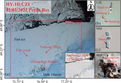
In this study, the CZI Level-1A data (digital number; DN; dimensionless) with a spatial resolution of 50 m were obtained from National Satellite Ocean Application Service (NSOAS), and the MSI Level-1C data (top-of-atmosphere reflectance, dimensionless) with a spatial resolution of 10 m were obtained from the European Space Agency (ESA). Both of them provide precise observation geometry data, including the solar zenith angle (θ₀), sensor zenith angle (θ), and relative azimuth angle (φ). Due to the relatively low solar elevation, the shadows of icebergs are long on ice surface and can be observed in both CZI and MSI images (Figure 1(b) and 1(c)).

3. Methods

3.1. Shadow pixel index

Detection method of cloud shadows can provide reference for the extraction of iceberg shadows (Choi and Bindschadler 2004; Jin et al. 2012; Zhu, Wang, and Woodcock 2015). For area covered by iceberg shadow, the direct solar radiation can hardly be received, and the reflected radiation of the surrounding terrain is weak. Therefore, the received signal is mainly composed of scattered atmospheric radiation, and it is stronger with the shorter wavelength. Scattering in the blue band is stronger than that in the near-infrared (NIR) band. Based on this, the normalized shadow pixel index (NSPI) is defined as

(1) $\text{NSPI=}({\text{DN}}_{\text{NIR}}{\text{-DN}}_{\text{Blue}}\text{ /}\left({\text{DN}}_{\text{NIR}}{\text{+DN}}_{\text{Blue}}\right)$(1)

Regions with low NSPI values can be regarded as iceberg shadow. In this study, the threshold of NSPI is set as −0.6 for CZI and MSI images after experiment. In order to determine the shadow length, the image is rotated and the rotation angle is γ = 360° – ζ – η, for convenience where ζ is the longitude of the iceberg position and η is the solar azimuth angle. The first and end pixels of shadow along the north-south direction in the rotated image are regarded as the shadow formation point (SFP) and shadow edge point (SEP), respectively, and the distance between them is calculated as the shadow length.

3.2. Shadow-height model

The shadow length has been widely used to estimate building height (Irvin and Mckeown 1989; Kadhim and Mourshed 2018). In this study, this method is employed to extract the iceberg freeboard, and only the surface height is considered without the fast ice thickness. There exists a geometric relationship between iceberg freeboard (H) and shadow length (S) associated with the observation geometry (Figure 2) and can be classified into two cases: (1) satellite and the sun on the same side of the iceberg (0° < |φ| < 180°); (2) satellite and the sun on different sides of the iceberg (180° < |φ| < 360°). α and β refer to the sensor/solar elevation angle, respectively, and can be calculated as the complementary angle of the sensor/solar zenith angle (θ and θ₀).

Figure 2. Geometric relationship between iceberg freeboard (H) and shadow length (S). Note that this figure is in the perspective view, where point O, P, Q, and R are in the same plane representing the ice surface orthogonal to the iceberg.

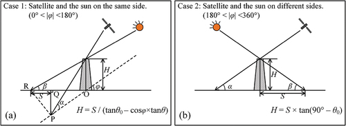
For the first case (Figure 2(a)), R is the edge point of shadow, P is the sensor observation point, O is the ground point of iceberg, and PQ is perpendicular to RO. Note that O, P, Q, and R are in the same plane representing the sea ice surface, and length of RQ represents the shadow length (S) in satellite images. According to the theory of cosine

(2) $\mathrm{R}{\mathrm{P}}^2=\mathrm{R}{\mathrm{O}}^2+\mathrm{P}{\mathrm{O}}^2-2\times \mathrm{RO}\times \mathrm{PO}\times \cos \mathit{\phi }$(2)

(3) $\mathrm{PO}=\mathit{H}/\tan \mathit{\alpha }=\mathit{H}\times \tan \mathit{\theta },\mathit{\hspace{0.17em}}\mathit{RO}\mathit{\hspace{0.17em}}=\mathit{H}/\tan \mathit{\beta }=\mathit{H}\times \tan {\theta }_0$(3)

(4) $\sin \mathrm{\angle }\mathrm{QRP}=\mathit{PQ}/\mathit{RP}=\mathit{PO}\times \mathit{sin\phi }/\mathit{RP}=\mathit{H}\times \mathit{tan\theta }\times \mathit{sin\phi }/\mathit{RP}$(4)

(5) $\cos \mathrm{\angle }\mathrm{QRP}=\mathrm{RQ}/\mathrm{RP}=\mathrm{S}/\mathrm{RP}$(5)

Squaring, adding, and making use of sin²∠QRP + cos²∠QRP = 1 gives

(6) $\mathit{H}=\mathit{S}/\left(\tan {\mathit{\theta }}_0-\mathrm{cos\phi }\times \mathrm{tan\theta }\right)$(6)

For the second case (Figure 2(b)), H can be calculated as

(7) $\mathit{H}=\mathit{S}\times \mathit{tan\beta }=\mathit{S}\times \mathit{tan}\left({90}^{\circ }-{\mathit{\theta }}_0\right)$(7)

The theoretical iceberg freeboard measurement precision (∆H) of a single shadow pixel and the absolute difference (AD) between the CZI-derived and MSI-derived results are acquired. They are defined as

(8) $\mathrm{\Delta }\mathit{H}=\mathrm{\Delta }\mathrm{L}\times \tan \mathit{\beta }$(8)

(9) $\mathrm{AD}=\left|{\mathit{H}}_{\_\mathrm{CZI}}-{\mathit{H}}_{\_\mathrm{MSI}}\right|$(9)

4. Results and discussion

4.1. Identification of iceberg shadows

Comparing the CZI image on 3 December 2022 and the MSI image on 6 December 2022, 66 pairs of icebergs with the size ranging from 0.005 to 2 km² were selected after filtering out the ones with incomplete shadows caused by neighboring icebergs and indistinguishable shadows caused by inaccurate determination of SFPs and SEPs. Considering the two images were obtained within 3 days, variation of the iceberg freeboard is relatively slight. Some of the selected iceberg pairs are shown in Figure 3.

Figure 3. Selected iceberg pairs in CZI (R: 650 nm, G: 560 nm; B: 460 nm) and MSI (R: 665 nm, G: 560 nm; B: 490 nm) true color RGB images. Note that some of them were on the track of ICESat-2 orbits (green dotted line) at the same period.

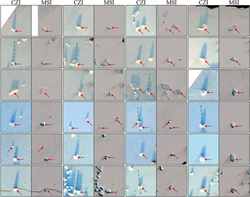
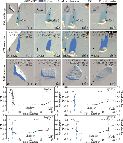
Iceberg shadows in CZI (case 1) and MSI (case 2) images correspond to the two cases in Section 3.2. Due to the very low sun elevation angle (2°) in CZI images, icebergs can form various shadows with different shapes, and the shadows can be sorted by shapes (Figure 4(a)), such as pinnacle, tabular, blocky, and wedge (Guan et al. 2021). The NSPI index advanced in this study can effectively distinguish these shadows in both CZI and MSI images (Figure 4(b)). NSPI values of iceberg shadows extracted along the artificial profile lines are significantly lower than those of icebergs and fast ice, showing a value response consistent with the spatial distribution of shadows, and the SFPs and SEPs can be extracted on these profile lines, which can be proved by the first-order derivatives as the two points are approximately equal to the breaking points of the NSPI curve (Figure 4(d)). In particular, for icebergs with irregular shadow shapes, the longest shadow along the north-south direction in the rotated image is considered corresponding to the highest point of the iceberg.

Figure 4. (a) CZI images showing different shapes of iceberg shadows, inset images are the corresponding MSI images. (b) and (c) NSPI extracted shadows in CZI and MSI images with the shadow orientation and observation geometry information annotated. Shadows in CZI images can be sorted by shapes, such as pinnacle, tabular, blocky, and wedge. (d) NSPI values and their first derivatives along the profile lines in (a). SFPs and SEPs are extracted and annotated on the profile lines.

4.2. Iceberg freeboard extraction and validation

66 pairs of icebergs were obtained in the study area and all of them can be observed and measured by both CZI and MSI images. Some key parameters of the selected icebergs are listed in Table 1. Distribution of the CZI and MSI derived iceberg freeboard is shown in Figure 5(a), and the distribution trend is basically consistent. Most of the icebergs are with a freeboard in the range of 30 to 80 m.

Figure 5. (a) Distribution of the iceberg freeboard (H) in CZI and MSI images. (b) The theoretical iceberg freeboard measurement precision (∆H) of a single shadow pixel in images with different spatial resolutions and solar elevation angles. (c) Distribution of the absolute difference (AD) of CZI-derived and MSI-derived iceberg freeboards. (d) Cross validation between the CZI-derived and MSI-derived iceberg freeboards.

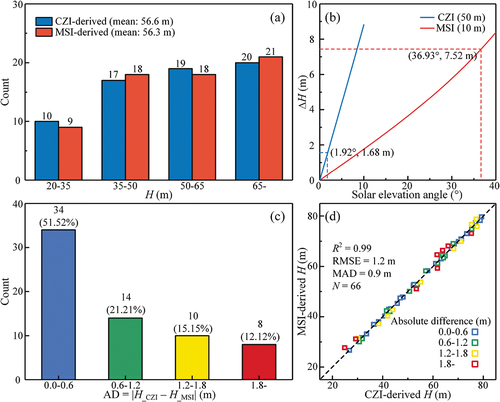
Table 1. Parameters of the selected icebergs in HY-1C/D CZI and Sentinel-2 MSI images.

Sensor	HY-1C/D CZI	Sentinel-2 MSI
Solar elevation angle	1.65°–2.20° (mean: 1.92°)	36.57°–37.37° (mean: 36.93°)
Length of shadows	656 m–4490 m	36 m–182 m
Iceberg freeboard	24.9 m–137.3 m (mean: 56.6 m)	26.7 m–137.1 m (mean: 56.3 m)

The precision evaluation results indicate that in optical images: (1) precisions of the iceberg freeboard are related to the pixel size (∆L) and solar elevation angle (β) (Figure 5(b)), and the low solar elevation of CZI image can effectively compensate for its lower spatial resolution; (2) the CZI-derived iceberg freeboards are highly correlated with the MSI-derived ones with a mean absolute difference (MAD) of 0.9 m ((Figure 5(d)), and more than half of the iceberg pairs (51.52%) are with an absolute difference (AD) less than 0.6 m (Figure 5(c)). For results derived from optical images, the MSI-derived ones are regarded as true values due to the higher spatial resolution. The measurement difference may come from: (1) mixed pixel effect caused by the different spatial resolution (50 m for the CZI image and 10 m for the MSI image), leading to the difficulty in determining the shadow boundary; (2) shadows in CZI and MSI images were on different sides of the iceberg, and the thickness of ice or snow on different sides was different.

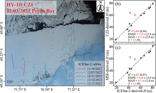
To further assess the measurement precision of optical images, the laser altimeter data from ICESat-2 was searched and checked. There were 5 tracks of ICESat-2 data covering the study area in the period of 15 days around the imaging date of CZI and MSI, where only 11 of 66 icebergs could be tracked by the ICESat-2 orbits due to the temporally incomplete and spatially sparse data coverage (Figure 6(a)). For ICESat-2, the iceberg freeboards could be extracted from Level-2A data (ATL03) processed by PhoREAL (version 3.30). Comparing the laser altimeter and optical satellite measurements (Figures 6(b) and 6(c)), the results indicate that the iceberg freeboard can be determined with acceptable precision (2 m) in optical images. It should be noted that there are two points (marked in red) where the ICESat-2-derived freeboards were significantly lower than the CZI or MSI derived ones, this is because the orbit track did not pass over the highest point of the iceberg, which is one major shortcoming of laser altimeter measurement.

Figure 6. (a) ICESat-2 orbits (from Nov 19, 2022 to Dec 15, 2022) overlaid on the icebergs in the study area. (b) and (c) Cross validation between the laser altimeter and optical satellite measurements of iceberg freeboards. Note that the parameters written in red included the outliers (orbit track did not pass over the highest point of the iceberg), while the parameters written in black did not include those points.

4.3. Estimation of iceberg basal melting

As the summer season in Antarctica (from October to next March) went on, the extent of fast ice in Prydz Bay changed significantly due to edge wasting, sidewall melting, and wave erosion. This can be observed in both CZI and MSI images on 25 January 2023 (Figure 7), where the outer edge of the fast ice turned out to have molten inwards for about 10 km. Apart from the disappeared icebergs on the melted or drifted fast ice, there remained 33 pairs of icebergs in the optical images on 25 January 2023. Some of them are shown in Figures 8(a),(b).

Figure 7. HY-1C CZI and Sentinel-2 MSI true color RGB images covering Prydz Bay on Jan 25, 2023, where the melting of fast ice can be observed. The enlarged and enhanced views of iceberg shadow are shown in the inset images.

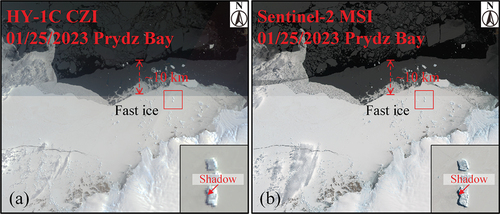
Figure 8. (a) and (b) Same-name icebergs in MSI images on Dec 06, 2022 and Jan 25, 2023. (b) Comparison of the freeboard derived on the two days. H’ (right y-axis) is defined as the absolute difference between the two.

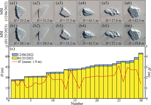
Optical images used in this study have the advantages of wide coverage and high temporal resolution, especially the HY-1C/D satellites which can ensure a global coverage twice a day. The wide coverage ensures that icebergs in the study area can all be observed, and the high temporal resolution ensures that the dynamic change of iceberg volume and freeboards can be measured. Therefore, basal melting of these icebergs can be estimated using repeated shadow measurements comparing with the results in Section 4.2. The mean solar elevation angles are 30° and 33° in CZI and MSI images on 25 January 2023, respectively. According to Equation 8(8) $\mathrm{\Delta }\mathit{H}=\mathrm{\Delta }\mathrm{L}\times \tan \mathit{\beta }$(8) , the theoretical freeboard measurement precision (∆H) of MSI image with higher spatial resolution is obviously better than that of CZI image. Estimating the freeboard of them by MSI images using the shadow-height method in Section 3, the results indicate that along with the iceberg drifting and rising temperature of Antarctic summer, the icebergs have experienced varying degrees of melting, and the freeboard of them have decreased in the range of 0.9 m to 3.1 m with a mean of 1.9 m (1 m/month during Antarctic summer) (Figure 8(c)), which is closed to the empirical results (0.8 m/month during the austral summer, Li et al. 2018) measured by the radar altimeter (i.e. CryoSat-2).

Unlike the satellite laser or radar altimeter which can only measure icebergs along the orbit tracks and rarely pass over a same iceberg, optical images can measure nearly all icebergs with wide coverage and high spatial and temporal resolution. Though suffering from cloud cover, the shadow-height method based on optical images can provide a good supplementary means for the altimeter method, which can help understand and quantify the mutual interaction between the environmental conditions (e.g. air temperature, ocean temperature, wind, etc.) and iceberg mass loss.

5. Conclusions

Iceberg shadow length can provide a reliable medium for estimating iceberg freeboard in optical images. This work presents a new methodological framework for the use of iceberg shadows with the following aspects: (1) identification of iceberg shadows; (2) determining iceberg freeboard using the shadow length; (3) estimating the basal melting of icebergs by repeated shadow measurements. So far, the methodological framework has been successfully applied to the HY-1C/D CZI and Sentinel-2 MSI images of icebergs in Prydz Bay, East Antarctica. The results of this work indicate that the normalized shadow pixel index (NSPI) is able to identify iceberg shadows with different shapes (i.e. pinnacle, tabular, blocky, and wedge). The shadow-height method can effectively estimate iceberg freeboard with non-overlapping shadow under different observation geometry conditions (satellite and the sun on the same or different sides), and the method has an acceptable precision (2 m) for optical images with high spatial resolution (<50 m). In addition to the spatial resolution, the performance of this method is mainly influenced by solar elevation, and the theoretical measurement precision is better with lower solar elevation. Moreover, basal melting of icebergs can be estimated based on repeated observations, for austral summer the melting rate is about 1 m/month, and the derived trend is in correspondence with the Antarctic seasonal trend. Compared with existing work utilizing shadow length to extract iceberg freeboard, in this work satellite images with different observation geometry conditions were taken into consideration, and iceberg basal melting can be estimated over successive time intervals. As a result, the methodological framework proposed in this work can measure nearly all icebergs with wide coverage and high spatial and temporal resolution and can provide a feasible supplementary means combined with the in-situ measured or satellite laser and radar altimeter data (e.g. Cryosat-2 and ICESat-2). Our future work will combine machine learning based techniques with this method to automatically extract the shadows and generate a high-quality freeboard dataset of the various icebergs in polar regions.

Acknowldgements

We thank the National Satellite Ocean Application Service (NSOAS, http://www.nsoas.org.cn/eng/), the European Space Agency (ESA, https://www.esa.int/) and the National Snow and Ice Data Center (NSIDC, https://nsidc.org/) for providing HY-1C/D, Sentinel-2 and ICESat-2 data, respectively. We particularly commemorate Dr. Jianqiang Liu for his contributions in popularizing the application of HY-1C/D satellites and guiding our research.

Disclosure statement

No potential conflict of interest was reported by the author(s).

Data availability statement

The data that support the findings of this study are available from the corresponding author, upon reasonable request.

Additional information

Funding

This work was jointly supported by National Key Research and Development Program of China [Grant number 2021YFC2803301], China Europe Dragon 5 Cooperation Program [Grant number 59310], and National Natural Science Foundation of China [Grant number 42071387].

Notes on contributors

Ziyi Suo

Ziyi Suo is currently a PhD student in Geography with Nanjing University and received his master’s degree with International Institute for Earth System Science, Nanjing University. His research interests include optical remote sensing of sea ice and ultraviolet remote sensing.

Yingcheng Lu

Yingcheng Lu is currently a Professor with International Institute for Earth System Science, Nanjing University. His research interests include optical quantitative remote sensing and its application in marine environment monitoring and treatment.

Jianqiang Liu

Jianqiang Liu was the Deputy Director with the National Satellite Ocean Application Service (NSOAS), Ministry of Natural Resources. His research interests include data preprocessing, satellite application, and sea ice monitoring.

Jing Ding

Jing Ding is currently a research scientist with the National Satellite Ocean Application Service (NSOAS), Ministry of Natural Resources. Her research interests include the assessment of the ocean satellite system and ocean remote sensing data processing.

Qing Wang

Qing Wang received his PhD degree in Geography with Nanjing University. His research interests include Lidar technology of monitoring marine environment.

Ling Li

Ling Li is currently a master student with International Institute for Earth System Science, Nanjing University. Her research interests include remote sensing data analysis and optical remote sensing of sea ice

Weimin Ju

Weimin Ju is currently a Professor with International Institute for Earth System Science, Nanjing University. His research interests include the retrieval of vegetation parameters from remote sensing data and simulating terrestrial carbon and water fluxes.

Manchun Li

Manchun Li is currently a Professor with the Jiangsu Provincial Key Laboratory of Geographic Information Science and Technology, Nanjing University. His research interests include geographic information system (GIS) and remote sensing applications.

References

- Benn, D. I., and J. A. Åström. 2018. “Calving Glaciers and Ice Shelves.” Advances in Physics 3 (1): 1. https://doi.org/10.1080/23746149.2018.1513819.
- Choi, H., and R. Bindschadler. 2004. “Cloud Detection in Landsat Imagery of Ice Sheets Using Shadow Matching Technique and Automatic Normalized Difference Snow Index Threshold Value Decision.” Remote Sensing of Environment 91 (2): 237–242. https://doi.org/10.1016/j.rse.2004.03.007.
- Dammann, D. O., L. E. B. Eriksson, S. V. Nghiem, E. C. Pettit, N. T. Kurtz, J. G. Sonntag, T. E. Busche, F. J. Meyer, and A. R. Mahoney. 2019. “Iceberg Topography and Volume Classification Using TanDEM-X Interferometry.” The Cryosphere 13 (7): 1861–1875. https://doi.org/10.5194/tc-13-1861-2019.
- Dryak, M. C., and E. M. Enderlin. 2020. “Analysis of Antarctic Peninsula Glacier Frontal Ablation Rates with Respect to Iceberg Melt-Inferred Variability in Ocean Conditions.” Journal of Glaciology 66 (257): 1–14. https://doi.org/10.1017/jog.2020.21.
- Enderlin, E. M., C. J. Carrigan, W. H. Kochtitzky, A. Cuadros, T. Moon, and G. S. Hamilton. 2018. “Greenland Iceberg Melt Variability from High-Resolution Satellite Observations.” The Cryosphere 12 (2): 565–575. https://doi.org/10.5194/tc-12-565-2018.
- Gladstone, R. M., G. R. Bigg, and K. W. Nicholls. 2001. “Iceberg Trajectory Modeling and Meltwater Injection in the Southern Ocean.” Journal of Geophysical Research Oceans 106 (C9): 19903–19915. https://doi.org/10.1029/2000jc000347.
- Guan, Z., X. Cheng, Y. Liu, T. Li, B. Zhang, and Z. Yu. 2021. “Effectively Extracting Iceberg Freeboard Using Bi-Temporal Landsat-8 Panchromatic Image Shadows.” Remote Sensing 13 (3): 430. https://doi.org/10.3390/rs13030430.
- Guo, G., L. Gao, J. Shi, and Y. Zu. 2022. “Wind-Driven Seasonal Intrusion of Modified Circumpolar Deep Water Onto the Continental Shelf in Prydz Bay, East Antarctica.” Journal of Geophysical Research Oceans 127 (12). https://doi.org/10.1029/2022JC018741.
- Irvin, R. B., and D. M. Mckeown. 1989. “Methods for Exploiting the Relationship Between Buildings and Their Shadows in Aerial Imagery.” IEEE Transactions on Systems, Man, and Cybernetics 19 (6): 1564–1575. https://doi.org/10.1109/21.44071.
- Jacobs, S. S., H. H. Helmer, C. S. M. Doake, A. Jenkins, and R. M. Frolich. 1992. “Melting of Ice Shelves and the Mass Balance of Antarctica.” Journal of Glaciology 38 (130): 375–387. https://doi.org/10.3189/S0022143000002252.
- Jansen, D., M. Schodlok, and W. Rack. 2007. “Basal Melting of A-38B: A Physical Model Constrained by Satellite Observations.” Remote Sensing of Environment 111 (2–3): 195–203. https://doi.org/10.1016/j.rse.2007.03.022.
- Jin, S., C. Homer, L. Yang, G. Xian, J. Fry, P. Danielson, and P. A. Townsend. 2012. “Automated Cloud and Shadow Detection and Filling Using Two-Date Landsat Imagery in the USA.” International Journal of Remote Sensing 34 (5): 1540–1560. https://doi.org/10.1080/01431161.2012.720045.
- Jongma, J. I., E. Driesschaert, T. Fichefet, H. Goosse, and H. Renssen. 2009. “The Effect of Dynamic-Thermodynamic Icebergs on the Southern Ocean Climate in a Three-Dimensional Model.” Ocean Modelling 26 (1–2): 104–113. https://doi.org/10.1016/j.ocemod.2008.09.007.
- Kadhim, N., and M. Mourshed. 2018. “A Shadow-Overlapping Algorithm for Estimating Building Heights from VHR Satellite Images.” IEEE Geoscience and Remote Sensing Letters 15 (1): 8–12. https://doi.org/10.1109/LGRS.2017.2762424.
- Li, T., M. Shokr, Y. Liu, X. Cheng, T. Li, F. Wang, and F. Hui. 2018. “Monitoring the Tabular Icebergs C28A and C28B Calved from the Mertz Ice Tongue Using Radar Remote Sensing Data.” Remote Sensing of Environment 216:615–625. https://doi.org/10.1016/j.rse.2018.07.028.
- Liu, Y., X. Cheng, R. M. Gladstone, J. N. Bassis, H. Liu, J. Wen, and F. Hui. 2015. “Ocean-Driven Thinning Enhances Iceberg Calving and Retreat of Antarctic Ice Shelves.” Proceedings of the National Academy of Sciences 112 (11): 3263–3268. https://doi.org/10.1073/pnas.1415137112.
- Li, T., B. Zhang, X. Cheng, M. J. Westoby, Z. Li, C. Ma, F. Hui, et al. 2019. “Resolving Fine-Scale Surface Features on Polar Sea Ice: A First Assessment of UAS Photogrammetry without Ground Control.” Remote Sensing 11 (7): 784. https://doi.org/10.3390/rs11070784.
- Merino, N., J. Le Sommer, G. Durand, N. C. Jourdain, G. Madec, P. Mathiot, and J. Tournadre. 2016. “Antarctic Icebergs Melt Over the Southern Ocean: Climatology and Impact on Sea Ice.” Ocean Modelling 104:99–110. https://doi.org/10.1016/j.ocemod.2016.05.001.
- Remy, J. P., S. Becquevort, T. G. Haskell, and J. L. Tison. 2008. “Impact of the B-15 Iceberg “Stranding event” on the Physical and Biological Properties of Sea Ice in McMurdo Sound, Ross Sea, Antarctica.” Antarctic Science 20 (6): 593–604. https://doi.org/10.1017/S0954102008001284.
- Rignot, E., S. Jacobs, J. Mouginot, and B. Scheuchl. 2013. “Ice Shelf Melting Around Antarctica.” Science 341 (6143): 266–270. https://doi.org/10.1126/science.1235798.
- Scambos, T., O. Sergienko, A. Sargent, D. MacAyeal, and J. Fastook. 2005. “ICESat Profiles of Tabular Iceberg Margins and Iceberg Breakup at Low Latitudes.” Geophysical Research Letters 32 (23): 97–116. https://doi.org/10.1029/2005GL023802.
- Schwarz, J. N., and M. P. Schodlok. 2009. “Impact of Drifting Icebergs on Surface Phytoplankton Biomass in the Southern Ocean: Ocean Colour Remote Sensing and In Situ Iceberg Tracking.” Deep Sea Research Part I: Oceanographic Research Papers 56 (10): 1727–1741. https://doi.org/10.1016/j.dsr.2009.05.003.
- Silva, T. A. M., G. R. Bigg, and K. W. Nicholls. 2006. “Contribution of Giant Icebergs to the Southern Ocean Freshwater Flux.” Journal of Geophysical Research 111 (C3): C03004. https://doi.org/10.1029/2004jc002843.
- Tamura, T., G. D. Williams, A. D. Fraser, and K. I. Ohshima. 2012. “Potential Regime Shift in Decreased Sea Ice Production After the Mertz Glacier Calving.” Nature Communications 3 (1): 826. https://doi.org/10.1038/ncomms1820.
- Tournadre, J., N. Bouhier, F. Girard-Ardhuin, and F. Rémy. 2015. “Large Icebergs Characteristics from Altimeter Waveforms Analysis.” Journal of Geophysical Research Oceans 120 (3): 1954–1974. https://doi.org/10.1002/2014JC010502.
- Tournadre, J., N. Bouhier, F. Girard-Ardhuin, and F. Rémy. 2016. “Antarctic Icebergs Distributions 1992-2014.” Journal of Geophysical Research Oceans 121 (1): 327–349. https://doi.org/10.1002/2015JC011178.
- Tournadre, J., F. Girard-Ardhuin, and B. Legrésy. 2012. “Antarctic Icebergs Distributions, 2002–2010.” Journal of Geophysical Research Oceans 117 (C5): C05004. https://doi.org/10.1029/2011JC007441.
- Wang, X., X. Cheng, P. Gong, C. K. Shum, D. M. Holland, and X. Li. 2014. “Freeboard and Mass Extraction of the Disintegrated Mertz Ice Tongue with Remote Sensing and Altimetry Data.” Remote Sensing of Environment 144:1–10. https://doi.org/10.1016/j.rse.2014.01.002.
- Williams, R. N., W. G. Rees, and N. W. Young. 1999. “A Technique for the Identification and Analysis of Icebergs in Synthetic Aperture Radar Images of Antarctica.” International Journal of Remote Sensing 20 (15–16): 3183–3199. https://doi.org/10.1080/014311699211697.
- Zhao, J., B. Cheng, T. Vihma, P. Lu, H. Han, and Q. Shu. 2022. “The Internal Melting of Landfast Sea Ice in Prydz Bay, East Antarctica.” Environmental Research Letters 17 (7): 074012. https://doi.org/10.1088/1748-9326/ac76d9.
- Zhu, Z., S. Wang, and C. E. Woodcock. 2015. “A Shadow-Overlapping Algorithm for Estimating Building Heights from VHR Satellite Images.” IEEE Geoscience & Remote Sensing Letters 15 (1): 8–12. https://doi.org/10.1109/LGRS.2017.2762424.