Forest age estimation using UAV-LiDAR and Sentinel-2 data with machine learning algorithms- a case study of Masson pine (Pinus massoniana)

ABSTRACT

The assessment of ecological functions, such as those of forest structure zoning and carbon sinks, heavily relies on forest age classification. Therefore, monitoring forest age is a crucial element of forest resource surveys. With the increased availability of high-quality open-access satellite data and advancements in Unmanned Aerial Vehicle Light Detection and Ranging (UAV-LiDAR) technology, remote sensing has emerged as an essential method for acquiring accurate forest age information. In this study, Sentinel-2 remote sensing data, UAV-LiDAR data, and combined Sentinel-2 and LiDAR data are used as data sources. Three machine learning algorithms, Adaptive Boosting (AdaBoost), Random Forest (RF), and Extreme Random Tree (ERT), are used to predict forest age in a Masson pine (Pinus massoniana Lamb.) forest. The optimal model is used to predict the forest age and simulate the spatial age distribution. The machine learning models based on separate Sentinel-2 and LiDAR data accurately predict the age of the Masson pine forest. Nevertheless, the accuracy of the RF model with combined data was higher than that in other cases, with an accuracy R value of 0.81. The model displayed good stability, and the spatial uncertainty of age estimation was low. Compared with the RF model using only Sentinel-2 data (R = 0.43), the RF model with combined LiDAR and Sentinel-2 data achieved the highest accuracy, with R values 88.37% higher. In addition, the forest canopy structure parameters, such as the average height of the forest stand extracted from UAV-LiDAR data, had a significant impact on the estimation of forest age. Thus, when the combined Sentinel-2 and LiDAR data were used to establish these parameters, the highest accuracy in the estimation of Masson pine was obtained. The findings of this study provide new insights for forest age estimation based on multi-source remote sensing data.

KEYWORDS:

• Masson pine
• forest age
• Unmanned Aerial Vehicle Light Detection and Ranging (UAV-LiDAR)
• Sentinel-2
• machine learning

1. Introduction

Forest age generally refers to the average age of a stand, which is a key factor in the evaluation of the ecological functions, such as the forest structure zoning and carbon sinks (Zhou et al. 2016). Related studies have shown that the Net Primary Productivity (NPP) of forest ecosystems increases rapidly with the growth of young stands, peaks at middle age, and declines slowly at maturity (Wang, Wang, and Yu 2008). Therefore, many carbon cycle models have considered the effect of stand age on NPP (He et al. 2012; Mao et al. 2022; Zheng et al. 2019). In addition, forest age is spatially heterogeneous, and its spatial distribution directly affects the forest biomass and species density (Eaton and Lawrence 2009; Hernández-Stefanoni et al. 2011). Therefore, forest age monitoring has been an important element in forest resource surveys and forest carbon sink function evaluations.

At present, forest age monitoring mainly consists of two methods: ground sample surveys and remote sensing estimations. The sample plot survey mainly uses the growth cones to measure the stand age or estimates the stand age by modeling the stand age with a stand diameter at breast height and tree height (Lu, Guo, and Hu 1993). This method obtains a real and reliable forest age, but it is time-consuming, laborious, and inefficient when applied to large-scale, extensive, or topographically complex forest areas, and it is difficult to obtain information such as the spatial distribution of forest age at the same time (Almeida et al. 2019). Remote sensing provides real-time, dynamic, simultaneous monitoring of large areas and information-rich data. Many optical remote sensing, Synthetic Aperture Radar (SAR), and Light Detection and Ranging (LiDAR) sensors offer temporally continuous and spatially consistent data products for forest resource monitoring. Therefore, combining remote sensing information with a small amount of forest age sample data to construct remote sensing information models for achieving large-scale spatial and temporal estimation of forest age application is an important technical tool for current forest age monitoring (Beckschäfer 2017; G. Chen et al. 2018; Kayitakire, Hamel, and Defourny 2006; Maltman et al. 2023).

Research suggests that as trees age, dynamic changes in the leaf chlorophyll content and internal structure significantly influence the spectral response. For example, leaves in the canopy of mature forests exhibit high contrast between near-infrared and red light reflectance (Grant 1987; Knipling 1970). Optical remote sensing can be used to acquire reflectance data for vegetation at different wavelengths, such as at visible spectral, near-infrared, and shortwave infrared wavelengths. These data can be used to calculate texture and various vegetation indices to monitor the growth of plants, making them the preferred data sources for monitoring forest age. Escasio, Santillan and Makinano-Santillan (2023) used Sentinel-2 images to establish a model to estimate the stand age of Falcata plantations, and they obtained satisfactory results. Spracklen and Spracklen (2021) also utilized Sentinel-2 images to classify the age of Acacia plantations, and the accuracy of their results met the relevant requirements. Li et al. (2018a) estimated the spatial distribution of the age of coniferous mixed forest, broad-leaved mixed forest, and coniferous mixed forest areas in the Haoer Mountain region using data such as Resource 3 satellite images. Li et al. (2022) utilized a Landsat time-series dataset from 1987 to 2019 covering Le County, Fujian, to establish a forest age estimation model that considers forest disturbances. They achieved high accuracy in estimating the forest age in highly disturbed areas.

However, optical remote sensing data do not provide to forest structure information, which may impact the accuracy of forest age estimation results. In contrast, LiDAR is a type of active remote sensing technology that is relatively less affected by weather conditions. It analyzes the magnitude, amplitude, frequency, and phase of the reflected spectrum on the surface of the ground object by measuring the propagation distance of the laser emitted from the sensor between the sensor and the target object. This analysis provides precise positioning information and presents accurate 3D-structural information of the target object (K. Zhou et al. 2022). Therefore, LiDAR has advantages in accurately estimating parameters such as forest canopy height, Leaf Area Index (LAI), storage volume, biomass, and carbon stocks (Jaskierniak et al. 2021; Mao et al. 2022; B. Zhang et al. 2022; Zhang et al. 2020; L. Zhou et al. 2022). Because tree height, crown width, and biomass being closely related to forest age, LiDAR data are an excellent data source for estimating forest age (Lefsky et al. 2005). For example, Racine et al. (2014) acquired forest structure and site attributes for natural forests in Canada using LiDAR data. They employed the k-nearest neighbor method to estimate the stand age of an entire forest area with high accuracy.

LiDAR data can be used to estimate stand age based solely on 3D structural information, but the absence of spectral information can lead to misclassification in stand age estimation. As a result, there has been growing interest in combining optical remote sensing data with LiDAR data to improve the estimation of forest age. Maltamo et al. (2009) predicted the age of managed forest areas in Finland with the nonparametric k-Most Similar Neighbor (k-MSN) method utilizing both Airborne Laser Scanning (ALS) data and aerial photographs, and good results were obtained. Xu, Manley and Morgenroth (2018) utilized RapidEye-derived metrics and LiDAR-derived metrics to forecast stand variables, such as mean top height, basal area, volume, and stand age, for planted forests in New Zealand. The estimation of stand age achieved the highest accuracy when combining RapidEye optical data with LiDAR data. Schumacher et al. (2020) used ALS and Sentinel-2 remote sensing variables in combination with the Norwegian Forest Resources Map stand index to develop a linear regression model for estimating the age map of forest stands in the Norwegian region. The findings of the study demonstrated that the tree height and stand index estimated by airborne laser scanning were the most crucial variables for predicting the stand age. Previous studies have demonstrated that combining optical remote sensing data with LiDAR data is efficient for predicting forest age. However, it has not been determined which combination method works best, therefore, it is necessary to compare the effectiveness of combining various data sources with models to estimate forest age at the regional scale (Xu, Manley, and Morgenroth 2018).

At present, the more widely used models for the quantitative estimation of remote sensing forest parameters mainly fall into two categories: statistical algorithms and machine learning algorithms. Statistical algorithms, such as the Multiple Linear Regression (MLR) model, have a simple structure and offer some advantages in estimating the forest biomass. However, the MLR model assumes a linear relationship between the remote sensing data and the biophysical attributes, as well as the independence of the remote sensing variables. In reality, most spectral responses of biophysical attributes are nonlinear, which means the MLR method often fails to meet the basic assumptions and cannot fully capture the intricate relationships between the remote sensing variables and the forest parameters (Du et al. 2012; Li et al. 2023). On the other hand, machine learning-based models such as Random Forest (RF), Support Vector Regression (SVR), Adaptive Boosting (AdaBoost), Gradient Boosting Decision Tree (GBDT), and Extreme Randomized Trees (ERT) models are able to reflect the nonlinear relationship between the remote sensing variables and the forest parameters with high parameter estimation accuracy. These models have become popular methodologies in the construction of remote sensing estimation models for forest parameters in recent years (Dong et al. 2020; Li et al. 2018). These methods are also being applied to forest age estimation. For instance, Tang et al. (2020) utilized Sentinel-2 images as the data source and employed the MLR, RF, and SVR methods to construct larch forest age estimation models. They achieved high accuracy in estimating the age of larch forests. Li (2022) used Landsat, Sentinel-2, and MODIS data as the base data and applied the RF, GBDT, and SVR algorithms to accurately estimate the monthly scale stand age in eucalyptus plantations.

In summary, optical remote sensing methods can be used to estimate forest age by acquiring spectral information, which is a widely used data source. Additionally, 3D structural information for forests obtained by LiDAR provides a new optional data source for forest age estimation. The purpose of this paper is to explore whether incorporating 3D structural information for forests into commonly used optical remote sensing datasets can improve the accuracy of forest age estimation. By combining the advantages of both optical and LiDAR remote sensing data, using machine learning methods for estimation means holds great potential in forest age remote sensing estimation research. This study combines ground data, remote sensing data and machine learning to estimate the age of a Masson pine forest. Specifically, we evaluate whether the combination of Sentinel-2 optical data and LiDAR data can improve the accuracy of forest age estimation compared with using either dataset alone. Additionally, three machine learning methods, namely AdaBoost, RF and ERT, are used to determine which method yields the highest accuracy and lowest error in estimating stand variables. This study provides new insights for forest age estimation and essential parameters for evaluating forest carbon income and expenditure.

2. Study area and data

2.1. Overview of the study area

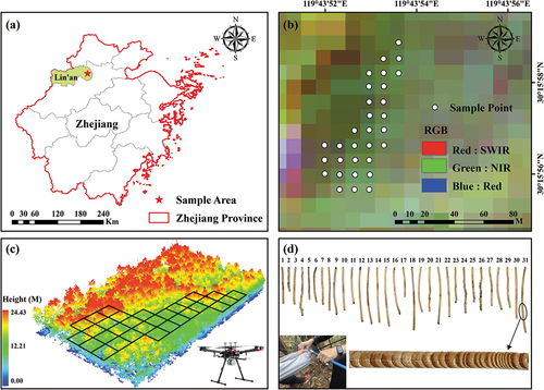
Lin’an is situated in the northwestern part of Zhejiang Province. It falls under the central subtropical monsoon climate zone, characterized by abundant precipitation and simultaneous periods of rain and warmth. The average annual temperature is approximately 16°C, with annual precipitation exceeding 1700 mm. The forest coverage rate in this region is remarkably high at 77.8%. The study area specifically lies in the eastern part of the Lin’an District, between 30°15’55″ and 30°16’00″ north latitude and 119°43’51″ and 119°43’55″ east longitude. The elevation of the area is approximately 102 m, making it a low mountainous region with a higher terrain in the east gradually sloping downward toward the west. The dominant tree species within the study area is Masson pine. Figure 1a displays the location information of the sample site.

Figure 1. (a) Location of the study area (b) spatial distribution of Sentinel-2 images and sample plots in the study area (c) UAV laser cloud images of study area sites (d) Masson pine age survey.

2.2. Datasets and processing

2.2.1. UAV-LiDAR data

A DJI Matrice 600 Pro hexacopter UAV with a lightweight lidar Velodyne Puck LITE^TM laser scanning instrument was utilized to collect the point cloud data in the study area on 18 October 2022, as shown in Figure 1c. The UAV operated at an altitude of 100 m, and followed a course spacing of 25 m. The data sampling implemented a collateral overlap rate of 50%. The laser wavelength used was 903 nm, accompanied by a laser emission frequency of 300 kHz. The sensor recorded the initial echo information from the laser pulse, employing a wavelength of 903 nm. It achieved a maximum scanning angle of ± 15°, a scanning frequency of 20 Hz, a scanning speed resulting in 300,000 points per second. The average point cloud density obtained was 190 points per square meter.

In the LiDAR360 platform, the LiDAR point cloud data were denoised using the height thresholding method. Subsequently, the ground and nonground points were extracted using the Improved Progressive TIN Densification (IPTD) filtering algorithm (Zhao et al. 2016). Triangulated Irregular Network (TIN) interpolation was then performed based on the ground points to generate Digital Elevation Models (DEMs) of the study area at a spatial resolution of 0.3 m. To account for the impact of topographic relief on the elevation values of the point cloud data, a normalization process was implemented, facilitating subsequent analysis.

2.2.2. Sentinel-2 data

Based on the ground survey data, a Sentinel-2 remote sensing image with low cloud cover and good quality was selected for performing the forest age estimation in the study area, as shown in Figure 1b. Sentinel-2 is equipped with 13 spectral bands, which include the visible, near-infrared, and short-wave infrared bands, along with its distinctive red-edge band. It has a swath width of 290 km and revisits the same area every 5 days. The spatial resolution of the obtained images is 10 m in the visible and near-infrared bands. The chosen image had the identifier N0400_R089_T50RQU, was captured on 30 September 2022, and had a cloud coverage of 2.05%. To analyze the selected image, it was imported into the Google Earth Engine (GEE) platform using the COPERNICUS/S2_SR_HARMONIZED dataset. Subsequently, cropping was performed to obtain a cloud-free image of the study area.

2.2.3. Masson pine age data collection

Before conducting aerial photography of the study area by UAV-LiDAR, this study established 31 fixed sample plots measuring 10 m × 10 m in the study area for performing a ground survey from 5 October 2022, to 18 October 2022, as shown in Figure 1b,c. The corners of each sample plot were accurately positioned using Real-Time Kinematics (RTK) with a horizontal positioning error of ±2 cm and an elevation positioning error of ±5 cm. During the ground survey, each sample plot was thoroughly examined. The total number of trees, along with their diameters at breast height, were recorded. Additionally, for each sample plot, five standard trees with different diameters and heights at breast height were carefully chosen. Growth cones were used to drill complete cores at breast height to determine the age of the trees by counting the annual rings, as depicted in Figure 1d. Subsequently, the collected cores were processed, and the average age of the standard trees was adopted as the average forest age of the sample plots. This average age served as the basis for constructing the subsequent forest age estimation model (Zhu et al. 2023).

3. Methods

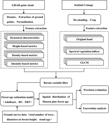
Three data sources, namely, LiDAR data, Sentinel-2 data, and the combination of LiDAR with Sentinel-2 data, were utilized to develop a model for estimating the forest age of Masson pine in the study area. Initially, remote sensing characteristic variables were defined based on relevant literature. Subsequently, the Boruta algorithm was utilized to analyze and select the significant variables for forest age estimation. To construct the forest age estimation model, three algorithms, namely, AdaBoost, RF, and ERT, were applied to the three data sources. Through accuracy assessments, the best model and data combinations was identified. The selected model and data combinations were then utilized for estimating the age distribution across the study area.

3.1. UAV-LiDAR data feature variable settings

The LiDAR data feature variables consisted of four categories: stand canopy structure features, stand height features, LiDAR point cloud density features, and LiDAR intensity. In total, there were 101 variables. Among these variables, the average tree height of each sample plot was determined by utilizing the DEM and DSM of the respective plot for segmenting the point cloud data into individual tree segments. The average height of the individual trees within the sample plot was then calculated. Detailed explanations of other parameters can be found in Table 1.

Table 1. LiDAR-extracted feature variables.

Feature Type	Feature Name	Feature Description
Structural characteristics	Height	Average stand height
	CC	Canopy Cover, Ratio of the number of vegetation points in the first echo to the number of points in the first echo.
	GF	Gap Fraction, Extract the number of ground points with Z-value below the height threshold (2m) divided by the total number of points
	LAI	Leaf Area Index, $\mathit{LAI}=-\frac{cos\left(\mathit{ang}\right)\times ln\left(\mathit{GF}\right)}{k}$, where ang is the mean scan angle, GF is the gap rate, and k is the extinction coefficient (Richardson, Moskal, and Kim 2009)
Height-based metrics	H1/H5/H10/H20/H25/H30/H40/H50/ H60/H70/H75/H80/H90/H95/H99	The percentiles of the canopy height distribution (1th, 5th, 10th, 20th,25th, 30th, 40th, 50th, 60th,70th,75th, 80th, 90th, 95th, and 99th) of first returns
	Hiq	Hiq = H75−H25。
	AIH1/AIH5/AIH10/AIH20/AIH25/ AIH30/AIH40/AIH50/AIH60/AIH70/AIH75/AIH80/AIH90/AIH95/AIH99	Cumulative percentile of canopy height distribution (1th, 5th, 10th, 20th,25th, 30th, 40th, 50th, 60th,70th,75th, 80th, 90th, 95th, and 99th) of first returns
	AIHiq	AIHiq = AIH75−AIH25。
	Hmax/Hmin/Hmean/Hmedia/Hmadme	Maximum height/minimum height/average height/median height/median absolute deviation of all points within each statistical cell
	Hvar/Hstdde/Hskew/Hkurt/Hcv/Hsqrt/ Hcurt/Hcanopy/Hmad	Variance/standard deviation/skewness/kurtosis/coefficient of variation/power-of-two average/power-of-three average/canopy undulation rate/mean absolute deviation for all point heights within each statistical unit
Density-based metrics	D0/D1/D2/D3/D4/D5/D6/D7/D8/D9	The proportion of points above the quantiles (10th, 20th, 30th, 40th, 50th, 60th, 70th, 80th, and 90th) to total number of points
Intensity-based metrics	I1/I5/I10/I20/I25/I30/I40/I50/I60/I70/I75/ I80/I90/I95/I99	The percentiles of the canopy intensity distribution (1th, 5th, 10th, 20th,25th, 30th, 40th, 50th, 60th,70th,75th, 80th, 90th, 95th, and 99th) of first returns
	Iiq	Iiq = I75−I25
	AII1/AII5/AII10/AII20/AII25/AII30/AII40 /AII50/AII60/AII70/AII75/AII80 /AII90/AII95/AII99	Cumulative percentile of canopy intensity distribution (1th, 5th, 10th, 20th,25th, 30th, 40th, 50th, 60th,70th,75th, 80th, 90th, 95th, and 99th) of first returns
	Imax/Imin/Imean/Imedia/Imadme	Median of the highest intensity/lowest intensity/average intensity/median intensity/median absolute deviation for all points within each statistical cell
	Ivar/Istdde/Iskew/Ikurt/Icv/Imad	Variance/standard deviation/skewness/kurtosis/coefficient of variation/mean absolute deviation for all point intensities within each statistical cell

3.2. Sentinel-2 remote sensing feature variable settings

Sentinel-2 remote sensing image feature variables were extracted, which can be categorized into three groups: spectral bands, vegetation indices, and texture features. These are detailed in Table 2:

Table 2. Sentinel-2 extracted feature variables.

Type	Name	Calculation Models or Descriptions	Abbreviation	Notes and References
Original Band	Aerosols	Band1	B1	/
	Blue	Band2	B2
	Green	Band3	B3
	Red	Band4	B4
	Red Edge 1	Band5	B5
	Red Edge 2	Band6	B6
	Red Edge 3	Band7	B7
	NIR	Band8	B8
	Red Edge 4	Band8A	B8A
	Water vapor	Band9	B9
	SWIR 1	Band11	B11
	SWIR 2	Band12	B12
Spectral Vegetation Indices	DVI	$\mathit{NIR}-\mathit{R}$	DVI	(Jaskierniak et al. 2021)
	EVI	$\left(2.5\left(\mathit{NIR}-\mathit{R}\right)\right)/\left(\mathit{NIR}+6\mathit{R}-7.5\mathit{B}+1\right)$	EVI	(Muhaimin et al. 2022)
	TVI	$0.5\left(120\left(\mathit{NIR}-\mathit{G}\right)-200\left(\mathit{R}-\mathit{G}\right)\right)$	TVI	(Su, Liu, and Su 2017)
	RVI	$\mathit{NIR}/\mathit{R}$	RVI	(Tan et al. 2019)
	PSRI	$\left(\mathit{R}-\mathit{B}\right)\times \mathit{RedEdge}2$	PSRI	(X. Zhang et al. 2022)
	NDII	$\left(\mathit{NIR}-\mathit{SWIR}1\right)/\left(\mathit{NIR}+\mathit{SWIR}1\right)$	NDII	(Sriwongsitanon et al. 2016)
	NDWI	$\left(\mathit{G}-\mathit{NIR}\right)/\left(\mathit{G}+\mathit{NIR}\right)$	NDWI	(Racine et al. 2014)
	NDVI	$\left(\mathit{NIR}-\mathit{R}\right)/\left(\mathit{NIR}+\mathit{R}\right)$	NDVI	(Muhaimin et al. 2022)
	MNDWI	$\left(\mathit{G}-\mathit{SWRI}1\right)/\left(\mathit{G}+\mathit{SWRI}1\right)$	MNDWI	(Qiu, Gan, and Zhao 2022)
	SAVI	$1.5\times \left(\mathit{NIR}-\mathit{R}\right)/\left(\mathit{NIR}+\mathit{R}+0.5\right)$	SAVI	(Zhen et al. 2021)
	NDBI	$\left(\mathit{SWIR}1-\mathit{NIR}\right)/\left(\mathit{SWIR}1+\mathit{NIR}\right)$	NDBI	(Muhaimin et al. 2022)
	Cire	$\left(\left(\mathit{RedEdge}3/\mathit{RedEdge}1\right)-1\right)$	Cire	(Gitelson, Gritz, and Merzlyak 2003)
Texture Features Based On The Gray-Level Co-occurrence Matrix (GLCM)	Variance	$\sum _{\mathit{i}=1}^n\sum _{\mathit{j}=1}^n{\left(\mathit{i}-\mathit{mean}\right)}^2{P}_{\mathit{ij}}$	VAR	$P_{\left(\mathit{i},\mathit{j}\right)}=\frac{{\mathit{V}}_{\left(\mathit{i},\mathit{j}\right)}}{{\sum }_{i=1}^n{\sum }_{j=1}^n{V}_{\left(\mathit{i},\mathit{j}\right)}}$ $V_{\left(\mathit{i},\mathit{j}\right)}$ is the $\mathit{i}$th row of the $\mathit{j}$th column in the $\mathit{N}$th moving window. $u_x=\sum _{\mathit{j}=1}^n\mathit{j}\sum _{\mathit{i}=1}^n{P}_{\left(\mathit{i},\mathit{j}\right)}$ $u_y=\sum _{\mathit{i}=1}^n\mathit{i}\sum _{\mathit{j}=1}^n{P}_{\left(\mathit{i},\mathit{j}\right)}$ ${\sigma }_x=\sum _{\mathit{j}=1}^n{\left(j-u_i\right)}^2\sum _{\mathit{i}=1}^n{P}_{\left(\mathit{i},\mathit{j}\right)}$ ${\sigma }_y=\sum _{\mathit{i}=1}^n{\left(i-u_j\right)}^2\sum _{\mathit{j}=1}^n{P}_{\left(\mathit{i},\mathit{j}\right)}$ (Li et al. 2023; Mohammadpour, Viegas, and Viegas 2022)
	Homogeneity	$\sum _{\mathit{i}=1}^n\sum _{\mathit{j}=1}^n\frac{1}{1+{\left(\mathit{i}-\mathit{j}\right)}^2}{P}_{\left(\mathit{i},\mathit{j}\right)}$	HOM
	Contrast	$\sum _{\left|\mathit{i}-\mathit{j}\right|=0}^{\mathit{n}-1}{\left|\mathit{i}-\mathit{j}\right|}^2\left\{\sum _{\mathit{i}=1}^n\sum _{\mathit{j}=1}^n{P}_{\left(\mathit{i},\mathit{j}\right)}\right\}$	CON
	Dissimilarity	$\sum _{\left|\mathit{i}-\mathit{j}\right|=0}^{\mathit{n}-1}\left|\mathit{i}-\mathit{j}\right|\left\{\sum _{\mathit{i}=1}^n\sum _{\mathit{j}=1}^n{P}_{\left(\mathit{i},\mathit{j}\right)}\right\}$	DIS
	Entropy	$-\sum _{\mathit{i}=1}^n\sum _{\mathit{j}=1}^n{P}_{\left(\mathit{i},\mathit{j}\right)}log\left(\mathit{P}\left(\mathit{i},\mathit{j}\right)\right)$	ENT
	Angular second moment	$\sum _{\mathit{i}=1}^n\sum _{\mathit{j}=1}^n\mathit{P}{\left(\mathit{i},\mathit{j}\right)}^2$	ASM
	Correlation	$\frac{{\sum }_{i=1}^n{\sum }_{j=1}^n\mathit{ij}{{\mathit{P}}_{\left(\mathit{i},\mathit{j}\right)}}^2-{\mu }_x{\mu }_y}{{\sigma }_x{\sigma }_y}$	COR
	Cluster Shade	$\sum _{\mathit{i}=1}^n\sum _{\mathit{j}=1}^n{\left(i+j-{\mu }_i-{\mu }_j\right)}^3{P}_{\left(\mathit{i},\mathit{j}\right)}$	SHA

1. The spectral bands are the grayscale values of the original bands of Sentinel-2 images.

2. The vegetation indices include the Difference Vegetation Index (DVI), Enhanced Vegetation Index (EVI), Triangular Vegetation Index (TVI), Ratio Vegetation Index (RVI), Plant Senescence Reflectance Index (PSRI), Normalized Difference Infrared Index (NDII), Normalized Difference Water Index (NDWI), Normalized Difference Vegetation Index (NDVI), Modified Normalized Difference Water Index (MNDWI), Soil Adjusted Vegetation Index (SAVI), Normalized Difference Barren Index (NDBI), and Chlorophyll Index (Cire).

3. Texture features are calculated by the grayscale co-generation matrix method for the four spectral bands of blue, green, red and near-infrared, including Variance (VAR), Homogeneity (HOM), Contrast (CON), Dissimilarity (DIS), Entropy (ENT), Angular Second Moment (ASM), Correlation (COR), Cluster Shade (SHA). To mitigate any biases caused by different texture window sizes (Zhao 2017), Gray-level Co-occurrence Matrix (GLCM) textures were calculated using window sizes of 3 × 3, 5 × 5, 7 × 7, 9 × 9, and 11 × 11. As a result, a total of 160 texture feature values, combined with 12 original band grayscale values and 12 vegetation indices, yielded a total of 184 remote sensing variables.

3.3. Boruta algorithm-based feature variable screening

The Boruta algorithm(Guindo et al. 2021b) is an RF-based classification wrapper algorithm that efficiently identifies features highly correlated with the outcome variable. It achieves this by building multiple RFs, creating shadow features that randomly rank the original features, and iteratively eliminating the original features. The Boruta feature selection algorithm screens out all features correlated with the dependent variable by iteratively eliminating variables whose importance is significantly lower than that of the shadow features (Marshall et al. 2023). The Z score is calculated by dividing the average accuracy loss by its standard deviation. The original feature is deemed important by comparing its Z score with the maximum Z score (MZSA) among the shadow features. If Z < MZSA, the feature is rejected; if Z > MZSA, the feature is accepted, and further statistical analysis is conducted using a two-sided test to determine its significance (Guindo et al. 2021a). The Boruta package in the R was used to filter the LiDAR data (Table 1) and the Sentinel-2 image features (Table 2).

3.4. Introduction to three machine learning models

3.4.1. Adaptive boosting algorithm

The AdaBoost algorithm, proposed by Freund and Schapire (1996) in 1996, aimed to improve the boosting algorithm, which is a popular combinatorial classifier approach. The AdaBoost algorithm works by training multiple weak classifiers on the same training set and then filtering them based on their weight coefficients to create a strong classifier. This iterative process results in a final classifier with a high accuracy for performing classification tasks. The sample weights are determined based on the correctness of each sample’s classification in every training iteration and the overall correctness of the final classification. Although the AdaBoost algorithm achieves high classification accuracy, it requires significant computational resources and involves a more complex process (Shu et al. 2015; Wang et al. 2013; Zhang 2018). In this study, we utilized the AdaBoostRegressor package from the ensemble module in the scikit-learn library to build an AdaBoost model for predicting the age of Masson pine.

3.4.2. Random forest

Breiman (2001) proposed the RF model by combining the bagging integrated learning algorithm (Breiman 1996) and the random subspace method (Ho 1998) and improved on the decision tree algorithm to propose the RF model, which can be used when the dependent variable is a categorical variable or a continuous variable. When the dependent variable is a categorical variable or a continuous variable, classification and regression analysis can be performed (Tang 2020), respectively. The RF algorithm employs bootstrap sampling to randomly select k samples from the original training set, where k is equal to the size of the training set. For each of the k samples, a decision tree model is built to obtain the k classification results. The final classification result is determined by voting on each record using the k classification results (L. Chen et al. 2018; Dong and Huang 2013; Fang et al. 2011). The RF model is straightforward to implement, provides good generalization capability, and operates much faster than the AdaBoost algorithm. In this study, the RandomForestRegressor package from the ensemble module in the scikit-learn library, implemented in the Python language, is used to construct a random forest model for predicting the age of Masson pine.

3.4.3. Extreme random trees

Proposed by Pierre Geurts in 2006, the ERT algorithm is an integrated learning algorithm that combines decision trees and is a variant of the RF model (Geurts, Ernst, and Wehenkel 2006). The ERT algorithm uses all of the training samples for training and randomly selects k features as split nodes to construct a decision tree consisting of k random nodes. By repeating this process N times, we obtain a classification model consisting of N decision trees. The final classification result is determined through voting (Wang, Tan, and Fan 2023). The key difference between the ERT and RF models lies in the sample selection: RF models adopt bootstrap sampling, while ERT models use all of the samples. Additionally, ERT models exhibit stronger randomness than RF models. Unlike RF models, which strive to find optimal nodes, ERT models obtain nodes completely at random (Wu et al. 2022). In this study, we constructed an ERT model to predict the age of Masson pine by utilizing the ExtraTreesRegressor package from the ensemble module in the scikit-learn library.

3.5. Model parameter adjustment

In this study, the GridSearchCV method is employed to tune the model parameters, and the performance of each parameter combination is evaluated based on 50-fold cross-validation. The optimization results of each model parameter are presented in Table 3.

Table 3. Optimized model parameters.

Model name	Parameter name	Parameter value
AdaBoost	n_estimators	250
	learning_rate	1
RF	n_estimators	50
	max_depth	10
	min_samples_split	10
	min_samples_leaf	1
ERT	n_estimators	5
	max_depth	10
	min_samples_split	2
	min_samples_leaf	4

3.6. Model accuracy evaluation method

Because of the small number of samples obtained, this study uses Leave One Out Cross-Validation (LOOCV) to verify the accuracy of the model to reduce the model error. LOOCV is a branch of K-fold CV, in which one sample is selected as the test set from N observed datasets, and the remaining N−1 samples are eliminated as the training set to build the model to obtain the prediction value of the test set. The operation is repeated N times until each sample is selected as the test set once (Wen, Zhao, and Huang 2022).

Two evaluation indices, the correlation coefficient R and the Root Mean Square Error (RMSE), are utilized to assess the estimation outcomes of the forest age model, which can better reflect the accuracy and stability of the model. The calculation equations are shown in Equations (1) and (2).

(1) $\mathit{R}=\sqrt{1-\frac{{\sum }_{i=1}^n{\left(\widehat{y_i}-y_i\right)}^2}{{\sum }_{i=1}^n{\left(y_i-\bar{y}\right)}^2}}$(1)

(2) $\mathit{RMSE}=\sqrt{\frac{{\sum }_{i=1}^n{\left(y_i-\widehat{y_i}\right)}^2}{\mathit{n}}}$(2)

where $y_i$ denotes the actual value of stand age, $\widehat{y_i}$ denotes the predicted value of stand age, $\bar{y}$ denotes the average value of stand age at all sample sites, and n denotes the number of sample sites.

The flowchart of this study is shown in Figure 2.

Figure 2. Flowchart of the steps used in our study.

4. Results and analysis

4.1. Feature variable screening and importance analysis

Figure 3a–d display the importance Z score for the four categories of LiDAR data: structural characteristics, height-based metrics, density-based metrics, and intensity-based metrics. Figure 3a–d indicate that no variables were selected for the intensity-based metrics, while 11 variables were selected among the three categories of structural characteristics, height-based metrics, and density-based metrics. Figure 3e–j illustrate the Z score for the three categories of the original band, vegetation index, and texture features of Sentinel-2 data. Variables such as B1, B5, B8A, B11 and B12 (original spectral bands) as well as variance, entropy, and shading (texture information) were selected.

Figure 3. Results of feature variable screening based on the Boruta algorithm.

Red box plots represent the Z scores of rejected features, and green box plots represent the Z scores of confirmed features. Yellow box plots indicate the Z scores of features that are yet to be determined. Blue box line plots correspond to the minimum, average, and maximum Z scores of shadow features. WiBjXX represents the texture information for the jth band window size of the image for i. XX refers to VAR, HOM, CON, DIS, ENT, ASE, COR, and SHA.

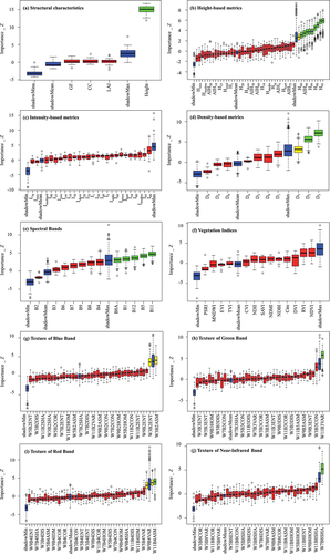
According to Figure 3, the average stand height obtained the highest score among all variables, with a Z score of approximately 15. Furthermore, height-based metrics such as H₉₅ also received high scores, which indicated their significant influence in estimating the age of Masson pine. In the Sentinel-2 data, the vegetation red-edge bands B5 and B8A, the shortwave infrared bands B11 and B12, and the shaded textures derived from B8 exhibited an effect on the age estimation of Masson pine.

Based on the above analysis, the variables listed in Table 4 were ultimately selected for the age estimation of Masson pine stands in this study. The LiDAR data included 12 variables, while the Sentinel-2 data included 8 variables.

Table 4. Feature variables filtered based on the Boruta algorithm.

Feature Types		Number	Feature Name
LiDAR parameter	Average stand height	1	Height
	Height-based metrics	9	AIH90/AIH95/AIH99/H5/H60/H80/H90/H95/H99
	Density-based metrics	2	D2/D3
Sentinel-2 parameter	Original Band	5	B1/B5/B8A/B11/B12
	GLCM	3	W9B3VAR/W9B4ENT/W5B8SHA

4.2. Comparison of forest age models with different data

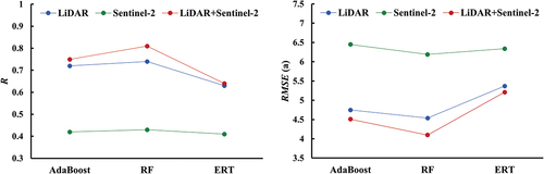
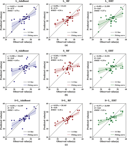
Figure 4 displays the R and RMSE of the age estimation for Masson pine after LOOCV cross-validation using three models from three data sources. The R of different models varied between 0.4 and 0.9, while the RMSE ranged from 6 to 10a. From a data source perspective, the combined LiDAR with Sentinel-2 forest age model exhibited the highest overall accuracy, followed by the LiDAR data alone and then the Sentinel-2 data alone. Compared to the least accurate Sentinel-2 data, the LiDAR data combined with the Sentinel-2 forest age model improved the R-value by 88.37% and reduced the RMSE value by 50.98%. Among the three machine learning models, the RF model generally outperformed the AdaBoost and ERT models in terms of accuracy. Specifically, the RF model constructed with LiDAR data combined with Sentinel-2 data achieved the highest accuracy, with an R of 0.81 and an RMSE of only 4.1 years. This corresponds to an 8% and 26.56% increase in accuracy compared to the AdaBoost and ERT models constructed with LiDAR data combined with Sentinel-2 data, respectively. Additionally, the RMSE is reduced by 10% and 27.07%, respectively.

Figure 4. Comparison of the accuracy of the forest age estimation models.

To further analyze the accuracy and distribution of misspecification in age models for Masson pine from three data sources, a correlation between the predicted and measured ages was plotted. Figures 5a–c depict the age models and prediction results of Masson pine based on single LiDAR data, single Sentinel-2 data, and LiDAR data combined with Sentinel-2 data, respectively. From Figure 5, it can be observed that the age of the Masson pine forest tended to be overestimated in all of the models between 25–40 years old, while the age of the Masson pine forest appears to be underestimated between 40–60 years old. Examining the deviation of the model fit curves from the 1:1 line reveals that the overestimation of lower values and underestimation of higher values are most pronounced for the single Sentinel-2 data, followed by the single LiDAR data, while the LiDAR data combined with the Sentinel-2 data shows relatively minimal deviations.

Figure 5. Forest age estimation results (a) accuracy evaluation of forest age model based on single LiDAR data (b) accuracy evaluation of forest age model based on single Sentinel-2 data (c) Accuracy evaluation of forest age model with LiDAR combined with Sentinel-2.

Table 5 presents the absolute values of each model’s prediction value and its corresponding actual value obtained through the difference operation. The cumulative percentage of the absolute prediction error values, $\left|\mathit{\epsilon }\right|\le 5\mathit{a}$, is calculated to analyze the error distribution of the forest age more precisely. Overall, the cumulative percentages of the absolute values of prediction errors$\left|\mathit{\epsilon }\right|\le 5\mathit{a}$ for the models based on the single Sentinel-2 data ranged from 0.58 to 0.61, which were generally low, indicating that the mean errors of the models based on the single Sentinel-2 data were larger, which was consistent with the results of Section 4.2. The cumulative percentage of the absolute value of prediction error$\left|\mathit{\epsilon }\right|\le 5\mathit{a}$ for the AdaBoost model based on the single LiDAR data is the highest at 0.87, followed by the ERT model based on the single LiDAR data and the AdaBoost and RF models of the LiDAR data combined with the Sentinel-2 data, both at 0.84, and the errors of several types of models are not very different. However, the number of prediction errors with an absolute value of$\left|\mathit{\epsilon }\right|=0$ for the RF model with LiDAR data combined with Sentinel-2 data is as high as 7, accounting for 22.58% of all samples, which is significantly higher than other models, and its stability is better.

Table 5. Distribution of the absolute values of prediction errors.

Data source – Models	The absolute value of prediction error (N = 31)
	0a	1a	2a	3a	4a	5a	>5a	$\mathit{\epsilon }\le 5$
S – AdaBoost	2	6	3	4	2	1	12	0.58
S – RF	4	5	1	5	2	2	11	0.61
S – ERT	3	4	5	1	3	3	12	0.61
L – AdaBoost	4	6	7	6	2	2	4	0.87
L – RF	2	7	5	6	2	3	6	0.81
L – ERT	4	4	5	5	4	4	9	0.84
S+L – AdaBoost	4	6	9	4	1	2	5	0.84
S+L – RF	7	3	6	3	4	3	5	0.84
S+L – ERT	1	6	4	7	2	3	8	0.74

In summary, LiDAR data combined with Sentinel-2 data and using the RF model can achieve accurate age estimation of Masson pine; of course, single LiDAR data also yield high accuracy in age estimation.

4.3. Prediction of the spatial distribution of the age of Masson pine

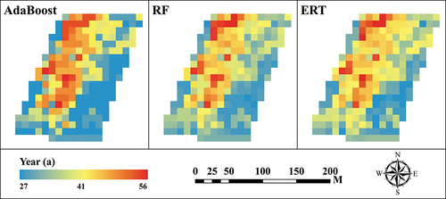
AdaBoost, RF, and ERT models were utilized to estimate the age of Masson pine stands using single LiDAR data, single Sentinel-2 data, and a combination of LiDAR data and Sentinel-2 data, respectively. The models were validated using the LOOCV method. The accuracy results indicated combining LiDAR with Sentinel-2 data and employing the RF model yielded the best solution for the age estimation of Masson pine. Building upon this finding, the study combined LiDAR and Sentinel-2 data to construct AdaBoost, RF, and ERT models for predicting the forest age of Masson pine in the Lin’an study area and its surrounding areas. Forest age distribution maps were obtained, and the results are presented in Figure 6. It is apparent that the age estimations from the three models for Masson pine stand in the study area ranged between 27 and 56 years, exhibiting a spatial distribution with higher values in the east and lower values in the west, as well as higher values in the north and lower values in the south.

Figure 6. Age distribution of Masson pine based on LiDAR combined with Sentinel-2 data.

5. Conclusion and discussion

5.1. Discussion

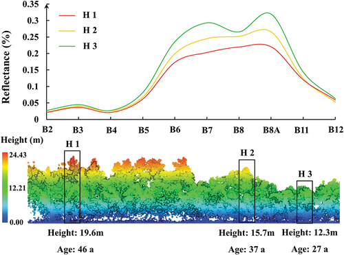
In this study, three data sources, LiDAR data, Sentinel-2 data, and a combination of LiDAR data and Sentinel-2 data, were used to construct an inverse model for estimating the age of Masson pine forests. The results indicated that the forest age model developed by combining LiDAR data with Sentinel-2 data exhibited higher accuracy than the models based solely on Sentinel-2 data or LiDAR data. This finding is consistent with the results reported by Xu, Manley and Morgenroth (2018), who also observed that a combined data model outperformed other models in terms of accuracy. Additionally, the RF model based on the combined data in this study achieved a higher accuracy (R = 0.81) than that of a larch stand age regression model based on Sentinel-2 (R = 0.79) as reported by Tang et al. (2020). Sentinel-2 data and other optical satellite remote sensing methods can be used to track vegetation growth through spectral features, vegetation indices, and texture analysis. Figure 7 clearly illustrates a significant disparity in the spectral reflectance of trees at different ages within the near-infrared and red-edge bands (703–864 nm) of the Sentinel-2 data. This discrepancy is evident as younger trees exhibit higher reflectance, and older trees display lower reflectance. The higher reflectance in younger trees can be attributed to their relatively smaller and sparser leaves, smaller thickness, and lower chlorophyll content. Conversely, as trees mature, their leaf density and thickness increase, along with higher chlorophyll content, resulting in decreased reflectance (Croft et al. 2013; Huang et al. 2023). However, optical remote sensing suffers from limitations such as spectral similarity and foreign bodies in the spectrum. This may lead to the phenomenon that young pine forests have the same spectra as old pine forests, or forests of the same age may have different spectra. Moreover, as natural stands of Masson pine approach a certain age (40–50 years)(Sun, Cao, and Sanchez-Azofeifa 2019; Zhang et al. 2004), their canopy closure leads to relatively uniform texture characteristics, further complicating accurate age estimation using Sentinel-2 data. In contrast, LiDAR data can provide precise information related to the forest age, including the stand height and the 3D canopy structure. As stands age, both the structure and density of trees undergo changes. For example, the increasing trend in tree height with increasing stand age is also reflected in Figure 7. The LiDAR-based variables in this study also encompass this information (Table 3), with point cloud height and canopy point cloud density increasing with increasing stand age. Overall, as stand age increases, spectral reflectance tends to decrease, trees grow taller, and the density of the canopy increases. Therefore, by combining LiDAR data and Sentinel-2 data, the advantages of both datasets are effectively leveraged, leading to accurate age estimation results.

Figure 7. Sentinel-2 spectral curves and normalized LiDAR point cloud heights for trees of different ages.

To avoid relying on a single model, three machine learning methods (AdaBoost, RF, and ERT) were used in this study for performing age estimation. The ensemble machine learning approach is adaptable to complex nonlinear relationships and can enhance the accuracy of forest age prediction by integrating multiple classifiers or decision trees. It continuously optimizes decision tools and strategies to maximize algorithm performance (Li et al. 2023). The RF is simple, easy to parallelize, capable of handling high-dimensional data, and exhibits good noise immunity (Breiman 2001; B. Zhang et al. 2022). AdaBoost is capable of handling high-dimensional data and large-scale features with low sensitivity to outliers. It also offers advantages in terms of speed, simplicity, and ease of programming (Tu, Liu, and Xu 2017). Extreme random trees have advantages in terms of training speed, memory consumption, and the handling of high-dimensional data, especially for large-scale datasets and high-dimensional feature spaces (Geurts, Ernst, and Wehenkel 2006). In this study, all three machine learning methods were found to be effective in estimating forest age. Among these methods, the RF model outperformed both the AdaBoost and ERT models in terms of accuracy. However, it is worth noting that the ERT model yielded lower accuracy results than the other two methods. Machine learning, especially integrated learning, is more advantageous for cases with many observed samples (Guo 2022; Yu et al. 2023; Zhang et al. 2022). For small sample sets, bootstrap sampling is more advantageous for model prediction. Both RF and AdaBoost utilize bootstrap sampling to construct the applied datasets. However, ERT employs a completely random sampling method, which may explain why the accuracy of RF and AdaBoost models is higher than that of the ERT model. Furthermore, RF demonstrates better robustness to noise and outliers, while AdaBoost is more sensitive to them, resulting in higher accuracy for the RF. The RF model demonstrated the highest performance in the forest age inversion study, which aligns with the findings of Tang et al. (2020). It is evident that the application of the random forest model in forest age estimation holds considerable promise.

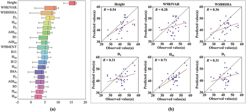
On the other hand, the modeling parameters greatly influence the accuracy and reliability of the forest age estimation model. Figure 8 demonstrates the correlation between the feature variables and forest age. In Figure 8a, the ranking of feature variables’ importance, filtered by Boruta’s algorithm, is illustrated. The average height of the forest stand shows the highest importance score (Z = 15.81), which is three times higher than the average importance of the other variables, making it the most significant parameter. It is followed by the green band variance with a window size of 9 × 9 (Z = 8.39) and the near-infrared band shadow with a window size of 5 × 5 (Z = 7.50) two texture features; LiDAR extracted the highest number of height variables (nine) and Sentinel-2 extracted spectral features (five), accounting for 45% and 25%, respectively, as key parameters for stand age estimation. Both the mean stand height and the height variables are indicators of the stand structure, confirming that the stand structure features have an important influence on the tree growth and stand age estimation. When the growth state and spatial structure of the forest change, the reflectance and texture information of the spectral bands in the remote sensing images will also change accordingly, so the spectral features and texture features can reflect the dynamic growth changes of the forest. To further understand the relationship between each parameter and the forest age, this study calculated the correlation between the variables screened by Boruta’s algorithm and the forest age using the RF model. Scatter plots of the top six variables with their respective importance scores and forest age were generated, as shown in Figure 8b. These plots show that all top six variables with importance scores are positively correlated with the stand age, with R values ranging from 0.28 to 0.71. Among them, the height where 95% of the points in the point cloud data cell (H95) are located and the average stand height (Height) exhibit the highest correlation coefficients of 0.71 and 0.54, respectively. This further confirms the close relationship between forest canopy parameters such as tree height and crown diameter in the RF model and stand age.

Figure 8. (a) Importance ranking of modeling parameters and (b) correlation between the top 6 variables in terms of importance ranking and stand age.

In this study, the UAV imagery of the study area was also acquired for comparison with Sentinel-2. The UAV imagery was captured by a DJI Phantom 4 Pro V2.0 drone equipped with a DJI FC6310 digital camera and acquired after processing. UAV imagery contains three spectral bands, blue, green and red. The texture features are calculated using the GLCM method in 3.2 for 3 spectral bands, yielding a total of 120 texture feature values. Plus 3 spectral band values and 4 visible vegetation indices (Table 6), for a total of 127 remotely sensed variables. Variables were averaged over the sample area.

Table 6. Visible vegetation index.

Name	Calculation Models	References
NGRDI	$\left(\mathit{G}-\mathit{R}\right)/\left(\mathit{G}+\mathit{R}\right)$	(Tucker 1979)
GLI	$\left(2\mathit{G}-\mathit{R}-\mathit{B}\right)/\left(2\mathit{G}+\mathit{R}+\mathit{B}\right)$	(Louhaichi, Borman, and Johnson 2001)
RGRI	$\mathit{R}/\mathit{G}$	(Deng et al. 2016)
ExG	$2\mathit{G}-\mathit{R}-\mathit{B}$	(W. Mao, Wang, and Wang 2003)

Figure 9a,b show the correlation plots between predicted and measured ages of RF forest age inversion models constructed on the basis of a single UAV imagery and LiDAR combined with UAV imagery, respectively, and show the accuracy R and error RMSE. From Figure 9a, it is evident that the accuracy of the RF model based on single UAV imagery (R = 0.18) is lower than the RF model accuracy based on single Sentinel-2 (R = 0.43) and single LiDAR (R = 0.74). And Figure 9b shows that the RF model accuracy of LiDAR combined with UAV imagery is R = 0.65, lower than that of LiDAR combined with Sentinel-2 (R = 0.81).

Figure 9. RF forest age model estimation results (a) accuracy evaluation of forest age model based on single UAV imagery data (b) accuracy evaluation of forest age model with LiDAR combined with UAV imagery.

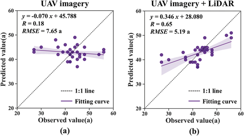
The results of RF model accuracy based on a single UAV imagery are less satisfactory for two main reasons: First, it is more difficult to account for changes in forest age using visible light data alone. None of the three visible bands of Sentinel-2 in Figure 3 were included. The difference in spectral reflectance of trees of different ages is not significant in the visible bands (B2-B4) of the Sentinel-2 data in Figure 7. So the UAV imagery inversion of forest age is not as accurate as Sentinel-2. Secondly, high spatial resolution imagery can capture detailed spectral-based information on individual trees. However, as UAV imagery is orthophoto, and there are instances of overlapping and interlocking tree canopies in densely forested areas, detailed spectral texture may introduce some uncertainty (Wen et al. 2020). In contrast, LiDAR can precisely acquire information such as stand height, which significantly influences forest age estimation (Figure 8). Therefore, the UAV imagery inversion of forest age is not as accurate as LiDAR. Furthermore, The negative correlation between UAV imagery data and forest age contributes to the reduced accuracy when combined with LiDAR data. Overall, combining LiDAR data with Sentinel-2 data yields better forest age inversion results.

The combination of Sentinel-2 and LiDAR is of great interest in small- and medium-scale forest age inversion. Of course, the use of UAV imagery data and LiDAR is also an important tool for forest age inversion, but with slightly less accuracy. For example, Maltamo et al. (2009) used ALS and aerial photographs to estimate stand attributes, including forest age, in managed forest areas in Finland. In Maltamo’s experimental results, the RMSE of the forest age result was 13.54–23.49 a, which was lower than the S+L result of the present study (RMSE of 4.1–5.21 a). Meanwhile, in our study, the RF model accuracy of LiDAR combined with UAV imagery has a lower accuracy. Investigating some sophisticated methodologies to further utilize UAV imagery may be able to improve forest age inversion accuracy(Brovkina et al. 2018; Qin et al. 2023; Ramli and Tahar 2020). In addition, although the satellite-based radar has lower resolution, it has better application prospects in large-scale forest age inversion by extracting tree heights and combining with Sentinel-2 (Zhou et al. 2023).

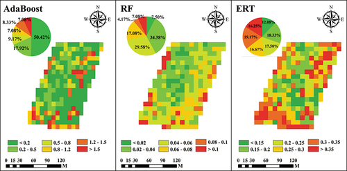
Uncertainty analysis assesses the accuracy of the forest age estimation by quantifying the degree of certainty (Li et al. 2023). The degree of uncertainty in the three models, namely, the AdaBoost, RF, and ERT models, based on LiDAR combined with Sentinel-2 data, was verified by calculating the standard deviation of the prediction results after 100 model runs, as shown in Figure 10. Figure 10 illustrates that the AdaBoost model exhibits a higher uncertainty range (0–3.2a) and greater model instability, followed by the ERT model (0–0.4 a), while the RF model demonstrates the smallest uncertainty range (0–0.14 a). To further analyze the frequency distribution of the model uncertainty, a pie chart was generated. It showed that 88.74% of the image elements with forest age uncertainty less than 0.08 a were accurately inverted using the RF model, which indicated its superior stability. Furthermore, the uncertainty distribution of all three models exhibited a trend of being low near the sample site and high in areas farther away from the sample site, which displayed significant spatial heterogeneity.

Figure 10. Uncertainty analysis of forest age prediction.

5.2. Conclusion

This study, three machine learning methods, namely AdaBoost, RF and ERT, are used to estimate the forest age based on three datasets: single LiDAR data, single Sentinel-2 data, and a combined dataset consisting of Sentinel-2 and LiDAR data. The study shows that: (1) the combined LiDAR data with the Sentinel-2 data model exhibited the highest overall accuracy, followed by the LiDAR data, and the Sentinel-2 data performed comparatively worse. (2) Regarding the LiDAR data combined with the Sentinel-2 data approach, all three machine learning models (AdaBoost, RF, and ERT) demonstrated reasonably accurate estimations of the upper Masson pine forest age. Among them, the RF model achieved the highest accuracy with an R of 0.81, minimal error, an RMSE of 4.1, and a low uncertainty in the spatial distribution of the forest age. (3) The forest canopy structure parameters, such as the mean stand height and the height characteristics extracted from the UAV-LiDAR data, significantly influenced the estimation of the forest age. This factor played a pivotal role in achieving high-precision estimation of the Masson pine age when combining the LiDAR data with the Sentinel-2 data. Combining the LiDAR data led to an 88.37% increase in the accuracy of the age estimation for the Masson pine compared to using the single Sentinel-2 data.

Disclosure statement

No potential conflict of interest was reported by the author(s).

Data availability statement

The Sentinel-2 dataset used in this study is publicly available for download from The Copernicus Open Access Hub (https://scihub.copernicus.eu/).The other data that support the findings of this study are available from the corresponding author, [Huaqiang Du, E-mail: [email protected]], upon reasonable request.

Additional information

Funding

This work was supported in part by the Leading Goose Project of Science Technology Department of Zhejiang Province [grant number 2023C02035], in part by the National Natural Science Foundation of China [grant number 32171785, 32201553 and 31901310], and in part by the Key Research and Development Program of Zhejiang Province [grant number 2021C02005].

Notes on contributors

Jinjin Chen

Jinjin Chen received the B.S. degree in geography information science from Zhejiang A & F University, Hangzhou, China, in 2021, where she is currently pursuing the M.S. degree. Her research interests include forest age and carbon storage estimation using remotely sensed data.

Xuejian Li

Xuejian Li received the B.S. degree in geographical science from Qiqihar University, Qiqihar, China, in 2014, and the M.S. degree in forest management and the Ph.D. degree in bamboo resources and efficient utilization from Zhejiang A & F University, Hangzhou, China, in 2017 and 2021, respectively. He is currently an Associate Professor with the School of Environment and Resources Science, Zhejiang A & F University. His research focuses on the temporal and spatial evolution of bamboo forest phenology and its response to climate change.

Zihao Huang

Zihao Huang received the B.S. degree in geographic information science from Nanjing Tech University, Nanjing, China, in 2018, and the M.S. degree in forest management from Zhejiang A & F University, Hangzhou, China, in 2021, where he is currently pursuing the Ph.D. degree in forestry. His research interests include land use and land cover change, machine learning, forest carbon estimation, and monitoring using remote sensing techniques.

Jie Xuan

Jie Xuan received the B.Eng. degree in Computer Science and Technology from Ningbo University, Ningbo, China, in 2020, the M.S. degree in Forestry from Zhejiang Agricultural and Forestry University, Hangzhou, China, in 2023, and is currently pursuing the Ph.D. degree in Forestry. His research interests include forest structure parameter extraction and biomass estimation, target detection, and forest carbon sink estimation.

Chao Chen

Chao Chen received the B.S. degree in geography information science from Zhejiang A & F University, Hangzhou, China, in 2021, where he is currently pursuing the M.S. degree. His research interests include the stand spatial structure using lidar data.

Mengchen Hu

Mengchen Hu received the B.S. degree in geography information science from Zhejiang A & F University, Hangzhou, China, in 2021, where she is currently pursuing the M.S. degree. Her research interests include phenology of urban forest and the effect of urbanization on it.

Cheng Tan

Cheng Tan received the B.S. degree in biological sciences from Zunyi Normal University, China, in 2021, where he is currently pursuing the M.S. degree.His research interests include the Masson pine pest monitoring.

Yongxia Zhou

Yongxia Zhou received the B.S. degree in forestry from Gansu Agricultural University, China, in 2021, where she is currently pursuing the M.S. degree. Her research interests include parameter estimation of moso bamboo forest based on UAV hyperspectral data.

Yinyin Zhao

Yinyin Zhao received the B.S. degree in surveying and mapping engineering from Zhejiang A & F University, Hangzhou, China, in 2022, where she is currently pursuing the M.S. degree. Her research interests include parameter extraction and biomass inversion of typical subtropical forests by UAV Live 3D and Satellite Remote Sensing.

Jiacong Yu

Jiacong Yu received the B.S. degree in geography information science from Zhejiang A & F University, Hangzhou, China, in 2022, where she is currently pursuing the M.S. degree. His research interests include the climate inversion and carbon cycle in subtropical forests.

Lei Huang

Lei Huang received her Bachelor’s degree in Land Resource Management from Jiangxi Agricultural University, Nanchang, China, in 2021. She is currently pursuing her master’s degree at Zhejiang Agriculture and Forestry University. Her research interests include the use of remote sensing data for monitoring land use change and estimating forest carbon stocks.

Meixuan Song

Meixuan Song received her Bachelor’s degree in agronomy from Jilin Agricultural University, Changchun, China, in 2022. She is currently pursuing her master’s degree at Zhejiang Agriculture and Forestry University. Her research interests include the use of remote sensing data for monitoring land use change and estimating forest carbon stocks.

Huaqiang Du

Huaqiang Du received the B.S. degree in forestry and the M.S. degree in forest management from Northeast Forestry University, Harbin, China, in 1999 and 2002, respectively, and the Ph.D. degree from Beijing Forestry University, Beijing, China, in 2005. He is currently a Professor with the School of Environment and Resources Science, Zhejiang A & F University, Hangzhou, China. His research interests include forest carbon estimation with remote sensing techniques and forest resource monitoring using multisource remotely sensed data and digital image processing.

References

- Almeida, D. R. A., S. C. Stark, R. Chazdon, B. W. Nelson, R. G. Cesar, P. Meli, E. B. Gorgens, et al. 2019. “The Effectiveness of Lidar Remote Sensing for Monitoring Forest Cover Attributes and Landscape Restoration.” Forest Ecology and Management 438:34–43. https://doi.org/10.1016/j.foreco.2019.02.002.
- Beckschäfer, P. 2017. “Obtaining Rubber Plantation Age Information from Very Dense Landsat TM & ETM+ Time Series Data and Pixel-Based Image Compositing.” Remote Sensing of Environment 196:89–100. https://doi.org/10.1016/j.rse.2017.04.003.
- Breiman, L. 1996. “Bagging Predictors.” Machine Learning 24 (2): 123–140. https://doi.org/10.1007/BF00058655.
- Breiman, L. 2001. “Random Forests.” Machine Learning 45 (1): 5–32. https://doi.org/10.1023/A:1010933404324.
- Brovkina, O., E. Cienciala, P. Surový, and P. Janata. 2018. “Unmanned Aerial Vehicles (UAV) for Assessment of Qualitative Classification of Norway Spruce in Temperate Forest Stands.” Geo-Spatial Information Science 21 (1): 12–20. https://doi.org/10.1080/10095020.2017.1416994.
- Chen, G., J.-C. Thill, S. Anantsuksomsri, N. Tontisirin, and R. Tao. 2018. “Stand Age Estimation of Rubber (Hevea Brasiliensis) Plantations Using an Integrated Pixel- and Object-Based Tree Growth Model and Annual Landsat Time Series.” ISPRS Journal of Photogrammetry and Remote Sensing 144:94–104. https://doi.org/10.1016/j.isprsjprs.2018.07.003.
- Chen, L., G. Zhou, H. Du, Y. Liu, F. Mao, X. Xu, X. Li, L. Cui, Y. Li, and D. Zhu. 2018. “Simulation of CO, Flux and Controlling Factors in Moso Bamboo Forest Using Random Forest Algorithm.” Scientia Silvae Sinicae 54 (8): 1–12. https://doi.org/10.11707/j.1001-7488.20180801.
- Croft, H., J. Chen, Y. Zhang, and A. Simic. 2013. “Modelling Leaf Chlorophyll Content in Broadleaf and Needle Leaf Canopies from Ground, CASI, Landsat TM 5 and MERIS Reflectance Data.” Remote Sensing of Environment 133:128–140. https://doi.org/10.1016/j.rse.2013.02.006.
- Deng, J., G. Ren, Y. Lan, H. Huang, and Y. Zhang. 2016. “Low Altitude Unmanned Aerial Vehicle Remote Sensing Image processing Based on Visible Band.” Journal of South China Agricultural University 37 (6): 16–22. https://doi.org/10.7671/j.issn.1001-11X.2016.06.003.
- Dong, L., H. Du, N. Han, X. Li, D. E. Zhu, F. Mao, M. Zhang, et al. 2020. “Application of Convolutional Neural Network on Lei Bamboo Above-Ground-Biomass (AGB) Estimation Using Worldview-2.” Remote Sensing 12 (6): 958. https://doi.org/10.3390/rs12060958.
- Dong, S., and Z. Huang. 2013. “A Brief Theoretical Overview of Random Forests.” Integration Techniques 2 (1): 1–7.
- Du, H., G. Zhou, H. Ge, W. Fan, X. Xu, W. Fan, and Y. Shi. 2012. “Satellite-Based Carbon Stock Estimation for Bamboo Forest with a Non-Linear Partial Least Square Regression Technique.” International Journal of Remote Sensing 33 (6): 1917–1933. https://doi.org/10.1080/01431161.2011.603379.
- Eaton, J. M., and D. Lawrence. 2009. “Loss of Carbon Sequestration Potential After Several Decades of Shifting Cultivation in the Southern Yucatán.” Forest Ecology and Management 258 (6): 949–958. https://doi.org/10.1016/j.foreco.2008.10.019.
- Escasio, J., J. Santillan, and M. Makinano-Santillan. 2023. “Using Machine Learning Classifiers and Regression Models for Estimating the Stand Ages of Falcata Plantations from Sentinel Data.” International Archives of the Photogrammetry, Remote Sensing and Spatial Information Sciences 48:465–472. https://doi.org/10.5194/isprs-archives-XLVIII-4-W6-2022-465-2023.
- Fang, K., J. Wu, J. Zhu, and B. Xie. 2011. “A Review of Random Forest Methods Research.” Statistics & Information Forum 26 (3): 32–38. https://doi.org/10.1007/3116(2011)03/0032/07.
- Freund, Y., and R. E. Schapire. 1996. “Game Theory, On-Line Prediction and Boosting.” Computational Learning Theory 325–332.
- Geurts, P., D. Ernst, and L. Wehenkel. 2006. “Extremely Randomized Trees.” Machine Learning 63 (1): 3–42. https://doi.org/10.1007/s10994-006-6226-1.
- Gitelson, A. A., Y. Gritz, and M. N. Merzlyak. 2003. “Relationships Between Leaf Chlorophyll Content and Spectral Reflectance and Algorithms for Non-Destructive Chlorophyll Assessment in Higher Plant Leaves.” Journal of Plant Physiology 160 (3): 271–282. https://doi.org/10.1078/0176-1617-00887.
- Grant, L. 1987. “Diffuse and Specular Characteristics of Leaf Reflectance.” Remote Sensing of Environment 22 (2): 309–322. https://doi.org/10.1016/0034-4257(87)90064-2.
- Guindo, M. L., M. H. Kabir, R. Chen, and F. Liu. 2021a. “Potential of Vis-NIR to Measure Heavy Metals in Different Varieties of Organic-Fertilizers Using Boruta and Deep Belief Network.” Ecotoxicology & Environmental Safety 228:112996. https://doi.org/10.1016/j.ecoenv.2021.112996.
- Guindo, M. L., M. H. Kabir, R. Chen, and F. Liu. 2021b. “Potential of Vis-NIR to Measure Heavy Metals in Different Varieties of Organic-Fertilizers Using Boruta and Deep Belief Network.” Ecotoxicology & Environmental Safety 228:112996. https://doi.org/10.1016/j.ecoenv.2021.112996.
- Guo, Y. 2022. Research on the Method of Forest Cover and ChangeInformation Extraction Based on Machine Learning. PhD diss., University of Chinese Academy of Sciences.
- He, L., J. M. Chen, Y. Pan, R. Birdsey, and J. Kattge. 2012. “Relationships Between Net Primary Productivity and Forest Stand Age in US Forests.” Global Biogeochemical Cycles 26 (3): 3. https://doi.org/10.1029/2010GB003942.
- Hernández-Stefanoni, J. L., J. M. Dupuy, F. Tun-Dzul, and F. May-Pat. 2011. “Influence of Landscape Structure and Stand Age on Species Density and Biomass of a Tropical Dry Forest Across Spatial Scales.” Landscape Ecology 26 (3): 355–370. https://doi.org/10.1007/s10980-010-9561-3.
- Ho, T. K. 1998. “The Random Subspace Method for Constructing Decision Forests.” IEEE Transactions on Pattern Analysis and Machine Intelligence 20 (8): 832–844. https://doi.org/10.1109/34.709601.
- Huang, Z., X. Li, H. Du, W. Zou, G. Zhou, F. Mao, W. Fan, Y. Xu, C. Ni, and B. Zhang. 2023. “An Algorithm of Forest Age Estimation Based on the Forest Disturbance and Recovery Detection.” IEEE Transactions on Geoscience Remote Sensing. https://doi.org/10.1109/TGRS.2023.3322163.
- Jaskierniak, D., A. Lucieer, G. Kuczera, D. Turner, P. N. J. Lane, R. G. Benyon, and S. Haydon. 2021. “Individual Tree Detection and Crown Delineation from Unmanned Aircraft System (UAS) LiDAR in Structurally Complex Mixed Species Eucalypt Forests.” ISPRS Journal of Photogrammetry and Remote Sensing 171:171–187. https://doi.org/10.1016/j.isprsjprs.2020.10.016.
- Kayitakire, F., C. Hamel, and P. Defourny. 2006. “Retrieving Forest Structure Variables Based on Image Texture Analysis and IKONOS-2 Imagery.” Remote Sensing of Environment 102 (3–4): 390–401. https://doi.org/10.1016/j.rse.2006.02.022.
- Knipling, E. B. 1970. “Physical and Physiological Basis for the Reflectance of Visible and Near-Infrared Radiation from Vegetation.” Remote Sensing of Environment 1 (3): 155–159. https://doi.org/10.1016/S0034-4257(70)80021-9.
- Lefsky, M. A., D. P. Turner, M. Guzy, and W. B. Cohen. 2005. “Combining Lidar Estimates of Aboveground Biomass and Landsat Estimates of Stand Age for Spatially Extensive Validation of Modeled Forest Productivity.” Remote Sensing of Environment 95 (4): 549–558. https://doi.org/10.1016/j.rse.2004.12.022.
- Li, M. 2022. Research on Estimation of Eucalyptus plantation Age in Guangxi Based on Time series Satellite Images. Master’s thesis., Guilin University of Technology.
- Li, X., H. Du, F. Mao, G. Zhou, L. Chen, L. Xing, W. Fan, et al. 2018. “Estimating Bamboo Forest Aboveground Biomass Using EnKF-Assimilated MODIS LAI Spatiotemporal Data and Machine Learning Algorithms.” Agricultural and Forest Meteorology 256–257:445–457. https://doi.org/10.1016/j.agrformet.2018.04.002.
- Li, F., M. Li, Z. Shi, H. Jiang, and J. An. 2018. “Estimates Stand Age Distribution Based on Forest Survey and Remote Sensing Data.” Forest Engineering 34 (2): 30–34. https://doi.org/10.16270/j.cnki.slgc.2018.02.019.
- Li, H., G. Zhang, Q. Zhong, L. Xing, and H. Du. 2023. “Prediction of Urban Forest Aboveground Carbon Using Machine Learning Based on Landsat 8 and Sentinel-2: A Case Study of Shanghai, China.” Remote Sensing 15 (1): 284. https://doi.org/10.3390/rs15010284.
- Li, Y., X. Zhou, Y. Chen, and F. Wang. 2022. “Estimation and Evaluation of Forest Age in Jiangle County, fujian Province Based on Lansat Time Series Remote Sensing Disturbance Detection.” Remote Sensing Technology and Applications 37 (3): 651–662. https://doi.org/10.11873/j.issn.1004-0323.2022.3.0651.
- Louhaichi, M., M. M. Borman, and D. E. Johnson. 2001. “Spatially Located Platform and Aerial Photography for Documentation of Grazing Impacts on Wheat.” Geocarto International 16 (1): 65–70. https://doi.org/10.1080/10106040108542184.
- Lu, Z., J. Guo, and S. Hu. 1993. “Determination of Stand Number Maturity Age by Growth Cone Sample Wood Method.” East China Forest Manager 7 (2): 29–33.
- Maltamo, M., P. Packalén, A. Suvanto, K. T. Korhonen, L. Mehtätalo, and P. Hyvönen. 2009. “Combining ALS and NFI Training Data for Forest Management Planning: A Case Study in Kuortane, Western Finland.” European Journal of Forest Research 128 (3): 305–317. https://doi.org/10.1007/s10342-009-0266-6.
- Maltman, J. C., T. Hermosilla, M. A. Wulder, N. C. Coops, and J. C. White. 2023. “Estimating and Mapping Forest Age Across Canada’s Forested Ecosystems.” Remote Sensing of Environment 290:113529. https://doi.org/10.1016/j.rse.2023.113529.
- Mao, F., H. Du, G. Zhou, J. Zheng, X. Li, Y. Xu, Z. Huang, and S. Yin. 2022. “Simulated Net Ecosystem Productivity of Subtropical Forests and its Response to Climate Change in Zhejiang Province, China.” Science of the Total Environment 838:155993. https://doi.org/10.1016/j.scitotenv.2022.155993.
- Mao, W., Y. Wang, and Y. Wang. 2003. “Real-Time Detection of Between-Row Weeds Using Machine Vision.” 2003 ASAE Annual Meeting, 1. St. Joseph: American Society.
- Marshall, T. L., L. C. Nickels, P. W. Brady, E. J. Edgerton, J. J. Lee, and P. A. Hagedorn. 2023. “Developing a Machine Learning Model to Detect Diagnostic Uncertainty in Clinical Documentation.” Journal of Hospital Medicine 18 (5): 405–412. https://doi.org/10.1002/jhm.13080.
- Mohammadpour, P., D. X. Viegas, and C. Viegas. 2022. “Vegetation Mapping with Random Forest Using Sentinel 2 and GLCM Texture Feature—A Case Study for Lousã Region, Portugal.” Remote Sensing 14 (18): 4585. https://doi.org/10.3390/rs14184585.
- Muhaimin, M., D. Fitriani, S. Adyatma, and D. Arisanty. 2022. “Mapping Build-Up Area Density Using Normalized Difference Built-Up Index (Ndbi) and Urban Index (Ui) Wetland in the City Banjarmasin.” IOP Conference Series: Earth and Environmental Science 1089 (1): 012036.
- Qin, S., H. Wang, X. Li, J. Gao, J. Jin, Y. Li, J. Lu, et al. 2023. “Enhancing Landsat Image Based Aboveground Biomass Estimation of Black Locust with Scale Bias-Corrected LiDAR AGB Map and Stratified Sampling.” Geo-Spatial Information Science 1–14. https://doi.org/10.1080/10095020.2023.2249042.
- Qiu, M., S. Gan, and L. Zhao. 2022. “Analysis of Index Method for Extracting Water Area of Erhai Lake Using Sentinel-2 Lmage.” Urban Geotechnical Investigation & Surveying 6:117–122. https://doi.org/10.1672/8262(2022)06-117-06.
- Racine, E. B., N. C. Coops, B. St-Onge, and J. Bégin. 2014. “Estimating Forest Stand Age from LiDAR-Derived Predictors and Nearest Neighbor Imputation.” Forest Science 60 (1): 128–136. https://doi.org/10.5849/forsci.12-088.
- Ramli, M. F., and K. N. Tahar. 2020. “Homogeneous Tree Height Derivation from Tree Crown Delineation Using Seeded Region Growing (SRG) Segmentation.” Geo-Spatial Information Science 23 (3): 195–208. https://doi.org/10.1080/10095020.2020.1805366.
- Richardson, J. J., L. M. Moskal, and S. H. Kim. 2009. “Modeling Approaches to Estimate Effective Leaf Area Index from Aerial Discrete-Return LIDAR.” Agricultural and Forest Meteorology 149 (6–7): 1152–1160. https://doi.org/10.1016/j.agrformet.2009.02.007.
- Schumacher, J., M. Hauglin, R. Astrup, and J. Breidenbach. 2020. “Mapping Forest Age Using National Forest Inventory, Airborne Laser Scanning, and Sentinel-2 Data.” Forest Ecosystems 7 (1): 793–806. https://doi.org/10.1186/s40663-020-00274-9.
- Shu, Y., S. Li, J. Li, H. Tang, X. Shi, and H. Du. 2015. “Classification of High Resolution Remote Sensing Image by CombiningSpatially Correlated Pixels Template and Multi-Class AdaBoost.” Remote Sensing Information 30 (4): 115–120. https://doi.org/10.3969/i.issn.1000-3177.2015.04.020.
- Spracklen, B., and D. V. Spracklen. 2021. “Synergistic Use of Sentinel-1 and Sentinel-2 to Map Natural Forest and Acacia Plantation and Stand Ages in North-Central Vietnam.” Remote Sensing 13 (2): 185. https://doi.org/10.3390/rs13020185.
- Sriwongsitanon, N., H. Gao, H. H. Savenije, E. Maekan, S. Saengsawang, and S. Thianpopirug. 2016. “Comparing the Normalized Difference Infrared Index (NDII) with Root Zone Storage in a Lumped Conceptual Model.” Hydrology and Earth System Sciences 20 (8): 3361–3377. https://doi.org/10.5194/hess-20-3361-2016.
- Su, T., Q. Liu, and X. Su. 2017. “Remote Sensing Classification of Crops Based on Multiple Vegetation Indices Time Series with Machine Learning.” Jiangsu Agricultural Sciences 45 (16): 219–224. https://doi.org/10.15889/j.issn.1002-1302.2017.16.054.
- Sun, C., S. Cao, and G. A. Sanchez-Azofeifa. 2019. “Mapping Tropical Dry Forest Age Using Airborne Waveform LiDAR and Hyperspectral Metrics.” International Journal of Applied Earth Observation and Geoinformation 83:101908. https://doi.org/10.1016/j.jag.2019.101908.
- Tang, S. 2020. Study on Extraction of Stand Age Information of Typical coniferous Forests in Northeast China and its Impact On tree Species Classification. Master’s thesis., Nanjing University.
- Tang, S., Q. Tian, K. Xu, N. Xu, and J. Yue. 2020. “Age Information Retrieval of Larix Gmelinii Forest Using Sentinel-2 Data.” Journal of Remote Sensing (Chinese) 24 (12): 1511–1524. https://doi.org/10.11834/jrs.20208500.
- Tan, Y., J. Y. Sun, B. Zhang, M. Chen, Y. Liu, and X. D. Liu. 2019. “Sensitivity of a Ratio Vegetation Index Derived from Hyperspectral Remote Sensing to the Brown Planthopper Stress on Rice Plants.” Sensors 19 (2): 375. https://doi.org/10.3390/s19020375.
- Tucker, C. J. 1979. “Red and Photographic Infrared Linear Combinations for Monitoring Vegetation.” Remote Sensing of Environment 8 (2): 127–150. https://doi.org/10.1016/0034-4257(79)90013-0.
- Tu, C., H. Liu, and B. Xu. 2017. “AdaBoost Typical Algorithm and its Application Research.” MATEC Web of Conferences, 00222. Vol. 139. Paris: EDP Sciences.
- Wang, X., L. Tan, and J. Fan. 2023. “Performance Evaluation of Mangrove Species Classification Based on Multi-Source Remote Sensing Data Using Extremely Randomized Trees in Fucheng Town, Leizhou City, Guangdong Province.” Remote Sensing 15 (5): 1386. https://doi.org/10.3390/rs15051386.
- Wang, X., C. Wang, and G. Yu. 2008. “Spatial and Temporal Patterns of Forest Carbon Exchange Based on Global Eddy Correlation.” China Science (Series D: Earth Science) 38 (9): 1092–1102.
- Wang, K., R. Zhang, D. Yin, and H. Zhang. 2013. “Cloud Detection for Remote Sensing Image Based on Edge Features and AdaBoost Classifier.” Remote Sensing Technology and Applications 28 (2): 263–268. https://doi.org/10.11873/j.issn.1004-0323.2013.2.263.
- Wen, X., M. Jia, X. Li, Z. Wang, C. Zhong, and E. Ma. 2020. “Identification of Mangrove Canopy Species Based on Visible Unmanned Aerial Vehicle Images.” Journal of Forest and Environment 40 (5): 486–496. https://doi.org/10.13324/j.cnki.jfcf.2020.05.005.
- Wen, B., L. Zhao, and L. Huang. 2022. “Proof of the Asymptotic Equivalence Between AlC Criterion and LOOCV.” Statistics & Decision 38 (6): 40–43. https://doi.org/10.13546/j.cnki.tjyjc.2022.06.008.
- Wu, S., J. Chen, L. Li, C. Zhang, R. Huang, and Q. Zhang. 2022. “Quantitative Inversion of Lunar Surface Chemistry Based on Hyperspectral Feature Bands and Extremely Randomized Trees Algorithm.” Remote Sensing 14 (20): 5248. https://doi.org/10.3390/rs14205248.
- Xu, C., B. Manley, and J. Morgenroth. 2018. “Evaluation of Modelling Approaches in Predicting Forest Volume and Stand Age for Small-Scale Plantation Forests in New Zealand with RapidEye and LiDAR.” International Journal of Applied Earth Observation and Geoinformation 73:386–396. https://doi.org/10.1016/j.jag.2018.06.021.
- Yu, Y., H. Gao, S. Tao, and S. Wang. 2023. “A Review of Hyperspectral Remote Sensing Image Classification Based on Ensemble Learnino.” Geomatics & Spatial Information Technology 46 (4): 49–52+60.
- Zhang, M. 2018. Research of the Detection Algorithm on Railway Fastener DefectsBased on Adaboost. Master’s thesis., Lanzhou Transportation University.
- Zhang, Z., L. Cao, H. Liu, X. Fu, and X. Shen. 2020. “Assessing the 3-D Structure of Bamboo Forests Using an Advanced Pseudo-Vertical Waveform Approach Based on Airborne Full-Waveform LiDAR Data.” IEEE Transactions on Geoscience & Remote Sensing 59 (12): 10647–10670. https://doi.org/10.1109/TGRS.2020.3042790.
- Zhang, X., X. Hou, M. Wang, L. Wang, and F. Liu. 2022. “Study on Relationship Between Photosynthetic Rate and Hyperspectral Indexes of Wheat Under Stripe Rust Stress.” Spectroscopy and Spectral Analysis 42 (3): 940–946. https://doi.org/10.3964/j.issn.1000-0593(2022)03-0940-07.
- Zhang, B., X. Li, H. Du, G. Zhou, F. Mao, Z. Huang, L. Zhou, J. Xuan, Y. Gong, and C. Chen. 2022. “Estimation of Urban Forest Characteristic Parameters Using UAV-Lidar Coupled with Canopy Volume.” Remote Sensing 14 (24): 6375. https://doi.org/10.3390/rs14246375.
- Zhang, Y., D. Lu, X. Jiang, Y. Li, and D. Li. 2022. “Forest Structure Simulation of Eucalyptus Plantation Using Remote-Sensing-Based Forest Age Data and 3-Pg Model.” Remote Sensing 15 (1): 183. https://doi.org/10.3390/rs15010183.
- Zhang, Q., G. Pavlic, W. Chen, R. Latifovic, R. Fraser, and J. Cihlar. 2004. “Deriving Stand Age Distribution in Boreal Forests Using SPOT VEGETATION and NOAA AVHRR Imagery.” Remote Sensing of Environment 91 (3–4): 405–418. https://doi.org/10.1016/j.rse.2004.04.004.
- Zhao, A. J. 2017. “Effects of Image Texture Window Sizes on LAle Estimation of Different Communities in Montane Broad-Leaved Forest.” Journal of Natural Resources 32 (5): 877–888. https://doi.org/10.11849/zrzyxb.20151266.
- Zhao, X., Q. Guo, Y. Su, and B. Xue. 2016. “Improved Progressive TIN Densification Filtering Algorithm for Airborne LiDAR Data in Forested Areas.” ISPRS Journal of PhotogrammetryRemote Sensing 117:79–91. https://doi.org/10.1016/j.isprsjprs.2016.03.016.
- Zhen, Z., S. Chen, T. Yin, E. Chavanon, N. Lauret, J. Guilleux, M. Henke, W. Qin, L. Cao, and J. Li. 2021. “Using the Negative Soil Adjustment Factor of Soil Adjusted Vegetation Index (Savi) to Resist Saturation Effects and Estimate Leaf Area Index (Lai) in Dense Vegetation Areas.” Sensors 21 (6): 2115. https://doi.org/10.3390/s21062115.
- Zheng, J., F. Mao, H. Du, X. Li, G. Zhou, L. Dong, M. Zhang, N. Han, T. Liu, and L. Xing. 2019. “Spatiotemporal Simulation of Net Ecosystem Productivity and Its Response to Climate Change in Subtropical Forests.” Forests 10 (8): 708. https://doi.org/10.3390/f10080708.
- Zhou, K., L. Cao, H. Liu, Z. Zhang, G. Wang, and F. Cao. 2022. “Estimation of Volume Resources for Planted Forests Using an Advanced LiDAR and Hyperspectral Remote Sensing.” Resources, Conservation and Recycling 185:106485. https://doi.org/10.1016/j.resconrec.2022.106485.
- Zhou, X., Y. Hao, L. Di, X. Wang, C. Chen, Y. Chen, G. Nagy, and T. Jancso. 2023. “Improving GEDI Forest Canopy Height Products by Considering the Stand Age Factor Derived from Time-Series Remote Sensing Images: A Case Study in Fujian, China.” Remote Sensing 15 (2): 467. https://doi.org/10.3390/rs15020467.
- Zhou, L., X. Li, B. Zhang, J. Xuan, Y. Gong, C. Tan, H. Huang, and H. Du. 2022. “Estimating 3D Green Volume and Aboveground Biomass of Urban Forest Trees by UAV-Lidar.” Remote Sensing 14 (20): 5211. https://doi.org/10.3390/rs14205211.
- Zhou, T., S. Wang, L. Zhou, Y. Chi, and M. Dai. 2016. “Carbon Dynamics of China’s Forests During 1901–2010: The Importance of Forest Age.” Chinese Science Bulletin 61 (18): 2064–2073. https://doi.org/10.1360/N972015-00811.
- Zhu, J., H. Shi, H. Sun, and R. Cong. 2023. “Some Thoughts on the Method of Measuring the Ages of Ancient Trees.” Chinese Landscape Architecture 39 (1): 124–127. https://doi.org/10.19775/j.cla.2023.01.0124.