Pan-tropical daily L-band microwave land surface emissivity retrieval from GNSS-R observations

ABSTRACT

The uncertainties in microwave land surface emissivity (MLSE) measurements have long limited the use of spaceborne microwave radiometer data. As an emerging observation method, Global Navigation Satellite System Reflectometry (GNSS-R) has demonstrated great potential in several land and ocean applications. In this study, a method for obtaining daily MLSE dataset in the pan-tropical region from Cyclone GNSS (CYGNSS) observations is presented and evaluated. The CYGNSS observations are first aggregated into the Equal-Area-Scalable-Earth (EASE) 2.0 36 km grid by a combined weight function of distance, time, and signal-to-noise ratio variance. Then, the method employs a pixel-by-pixel regression algorithm to conduct the daily MLSE retrieval using reference emissivity derived from the Soil Moisture Active Passive (SMAP) brightness temperature. The CYGNSS MLSE shows good agreement with SMAP MLSE, delivering an overall root-mean-square error (RMSE) of 0.022 and 0.017 for horizontal and vertical polarization, respectively, during the training set spanning the whole year of 2018. Furthermore, on the test set from January 2019 to May 2019, the RMSE values amounted to 0.030 and 0.023 for horizontal and vertical polarization, respectively. Temperature records from the International Soil Moisture Network are employed to calculate the emissivity and for in-situ validation, which yield an RMSE of 0.034 and 0.026 for the two polarizations, respectively. The proposed algorithm provides an encouraging approach to obtain accurate daily MLSE dataset for microwave remote sensing. Compared to the SMAP MLSE, the CYGNSS MLSE has a remarkable improvement of 86% in temporal resolution, greatly complementing the existing microwave emissivity datasets.

KEYWORDS:

• Microwave land surface emissivity (MLSE)
• Global Navigation Satellite System Reflectometry (GNSS-R)
• Cyclone GNSS (CYGNSS)

1. Introduction

Land surface emissivity (LSE) is a critical quantity in the knowledge of the surface thermal radiation and is significant for studying land physical processes (Min, Lin, and Li 2009; Wu et al. 2022; Zhang et al. 2023). Thermal infrared and microwave are the most concerned bands in the study of LSE. In comparison with thermal infrared, microwaves are capable of penetrating clouds and are less affected by the atmosphere for their longer wavelength. However, the application of microwave radiometry for land surface parameter retrievals is quite challenging due to the complexity compared to the ocean surface. The land parameters affecting microwave land surface emissivity (MLSE) mainly include soil moisture, roughness, soil type, vegetation, and surface water.

MLSE cannot be directly measured but can be retrieved from emission measurements such as spaceborne radiometers (Ringerud, Kummerow, and Peters-Lidard 2015). So far, many studies have retrieved MLSE using the top of atmosphere (TOA) microwave brightness temperatures from satellite sensors such as Special Sensor Microwave Imagers (SSM/I) (Prigent, Rossow, and Matthews 1997), Advanced Microwave Sounding Unit (AMSU) (Karbou et al. 2005), and Advanced Microwave Scanning Radiometer-Earth Observing System (AMSR-E) (Moncet et al. 2011; Norouzi et al. 2011). Statistical modeling is a commonly used empirical approach which looks at the statistical relationship between emissivity and predictor variables from historical data (Tian et al. 2015; Turk, Haddad, and You 2014). One of the simplest statistical modeling methods involves establishing a regression relationship between brightness temperature and emissivity. In addition, physical modeling is also a basic approach to estimate emissivity at a small scale, which employs numerical models to calculate emissivity based on their physical relationship with other land surface variables such as soil moisture, soil texture, and vegetation properties (Ringerud et al. 2013; Weng, Yan, and Grody 2001).

The uncertainty in MLSE greatly limits the use of spaceborne microwave radiometer data. Therefore, it is necessary to improve the existing emissivity acquisition methods (Wu et al. 2022). In the past few years, reflected signals from Global Navigation Satellite System (GNSS) have been found to be a signal of opportunity to observe the earth surface, and this technology is called the Global Navigation Satellite System-Reflectometry (GNSS-R) (Jing et al. 2024). The GNSS-R receiver is equipped with a configuration of bistatic radar, offering a low-cost observation approach with no need to transmit signals. At present, about 130 available GNSS satellites along with their abundant signal resources have the potential to provide observations with high spatial and temporal resolution (Jin, Wang, and Dardanelli 2022). Furthermore, the GNSS-R receiver can also be carried on ground and airborne platforms, providing a way to meet needs in different scenarios. The main observation of the GNSS-R receiver is the delay-Doppler map (DDM), which is created by cross correlating the received signal with a locally generated replica for different path delays and Doppler shifts. GNSS-R data have been used in several land and ocean applications, such as soil moisture retrieval (Chew and Small 2020; Dong and Jin 2021; Yan et al. 2020), forest biomass estimation (Zribi et al. 2019), sea ice detection (Alonso-Arroyo, Zavorotny, and Camps 2017) and sea wind speed retrieval (Chen et al. 2022; Li et al. 2023; Ruf et al. 2016; Saïd et al. 2021).

Compared to existing MLSE measurements, GNSS-R derived MLSE is advantageous as it does not rely on knowledge of surface temperature. The surface reflectivity is the main derivation from DDM on land. The electromagnetic scattering modeling for GNSS-R on rough surfaces is typically based on the Kirchhoff approximation, and the surface roughness is commonly decomposed into three scales: topographic, intermediate, and microwave scales. A recent study has presented a comparison between three electromagnetic scattering models (Campbell et al. 2022). In theory, for a perfectly flat interface between two homogeneous media, the sum of reflectivity and emissivity obtained with the same system is 1. However, for the rough land surface, the impinging GNSS signal is scattered not only in the specular direction but also in other directions. The GNSS-R receiver primarily tracks signals in the near-specular direction, while passive microwave radiometry observes the upper hemisphere. The two would only yield the same results if the surface was completely flat and devoid of diffused scattering. Thus, it is inappropriate to assume that microwave emissivity is simply one minus the GNSS-R reflectivity. Given the unique advantages of GNSS-R technology, the connection between GNSS-R reflectivity and microwave emissivity is valuable to discuss.

This work proposes a pixel-by-pixel method to obtain daily MLSE in the pan-tropical region from CYGNSS observations. This work aims to provide a new approach to complement the existing microwave emissivity datasets. This paper is structured as follows: Section 2 introduces the data used in this study. Section 3 describes the proposed daily MLSE retrieval model. Section 4 presents the results, both in the pan-tropical region and over the in-situ sites, and section 5 summarizes the conclusions.

2. Data

2.1. CYGNSS data

CYGNSS was launched on 15 December 2016 by NASA, and comprises eight low Earth orbit satellites. The signals observed are the Global Positioning System (GPS) L1 (1.58 Ghz) coarse-acquisition codes and eight satellites produce 32 measurements per second (increased to 64 measurements per second after July 2019). CYGNSS can monitor variations in the pan-tropical region (within ±38° latitudes). The determination of spatial resolution is still unsolved at present, as it depends on the roughness of the surface in the specular and near-specular directions. For coherent reflected signals over a smooth surface, a current consensus is that, the size of the footprint is defined by the first Fresnel zone. Thus, during the period of one CYGNSS measurement, the theoretical smallest area of ground is ~7 × 0.5 km (turned to ~3.5 × 0.5 km after July 2019) (Chew and Small 2018).

In this work, CYGNSS Level1 (L1) v2.1 data from January 2018 to December 2018 are used for model training, while data from January 2019 to May 2019 are used for test (CYGNSS 2017). The following criteria are used to filleted the CYGNSS data: 1) the maximum of analog power greater than −147, 2) the antenna gain greater than 0 dB 3) the incidence angle (i.e. the angle between the transmitter to specular point ray and the surface normal) less than 40°, 4) the maximum of analog power at a delay bin of 7–10, 5) the quality flags (possible low quality and low confidence in the GPS equivalent isotopically radiated power) provided by CYGNSS, and 6) the water mark described in section 2.4. The above criteria are concluded from the previous CYGNSS-based studies (Dong and Jin 2021; Eroglu et al. 2019; Yang et al. 2022), which can increase the reliability of CYGNSS observations.

2.2. SMAP data

The Soil Moisture Active Passive (SMAP) mission was developed by NASA and incorporated radar and radiometers to perform the earth observation missions (Entekhabi, Njoku, et al. 2010). Unfortunately, the radar failed in 2015, leaving the only operation of radiometer. The SMAP instruments operate at L band (1.41 GHz) and provide a conically scanning antenna beam with an incidence angle of 40°. In this work, gridded brightness temperature data at horizontal and vertical polarizations (H and V) from the SMAP L1C v005 product (Chan, Njoku, and Colliander 2020) and surface temperature data from the SMAP L3 v007 product (O’Neill et al. 2020) are used, which are stored in the form of Equal-Area-Scalable-Earth (EASE) 2.0 36 km grid. The brightness temperature data have been corrected for atmospheric effects, Faraday rotation, and low-level Radio Frequency Interference (RFI) effects. Products of descending half-orbit pass are employed here, at which time the soil, vegetation, and air are in approximate thermal equilibrium. This descending half-orbit data can help simplify the physical model and improve the accuracy of derived soil moisture estimations (Entekhabi, Njoku, et al. 2010). The surface temperature is derived from the Goddard Earth Observing System Model, Version 5 (GEOS-5), forward processing (FP) system and has been modified by the Choudhury two-layer approach (Entekhabi et al. 2010).

2.3. ISMN data

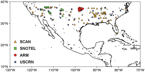
The International Soil Moisture Network (ISMN) was set up in 2009 with the objective of supporting global satellite products (Dorigo et al. 2011). ISMN stores a variety of in-situ hydrometeorological measurements such as soil moisture, temperature of soil and air, and precipitation. In this work, soil temperature records at 10 cm depth from 132 in-situ sites within the Continental United States (CONUS) are employed to calculate emissivity (Figure 1). The CYGNSS data within 0.15° (approximately 14 km) of each site are collected and aggregated using the weight function described in section 3.3 to calculate the effective reflectivity. The corresponding brightness temperature data are obtained by linear interpolation from the data of the nearest four grid nodes.

Figure 1. Distributions of selected in-situ sites from ISMN.

2.4. GSW data

The Global Surface Water (GSW) dataset, jointly developed by the European Joint Research Centre (JRC) and the United States Geological Survey (USGS), is a comprehensive and high-resolution collection of information that maps the occurrence, changes, and dynamics of Earth’s surface water bodies over the past three decades (Pekel et al. 2016). The “seasonality” data are employed in this work, which is available at https://global-surface-water.appspot.com. The spatial resolution of this product is about 30 m × 30 m, and each pixel indicates the duration of open water in a year (0–12). Since the water body has a significant impact on the GNSS-R and brightness temperature data, we employ the water body removal method (Yang et al. 2023) and do not perform retrievals in 36 km pixels with a percentage of 30 m water pixels greater than 10%.

3. Method

3.1. Land emissivity derivation from brightness temperature

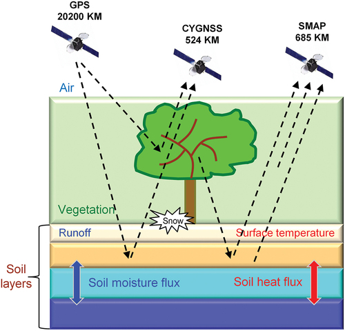
Derivation of emissivity from SMAP atmospherically corrected surface brightness temperature is founded on the radiative transfer equation commonly known as the $\mathit{\tau }-\mathit{\omega }$ model. The brightness temperature at the top of vegetation layer $\mathit{T}{B}^p$ for low frequencies can be modeled from emission components of soil and overlying vegetation canopy (Figure 2) (Jackson and Schmugge 1991):

Figure 2. Schematic of emission and GNSS-R reflectivity from vegetation and soil. Atmosphere contribution is not included here.

(1) $\mathit{T}{B}^p=T_s{e}^p{\gamma }^p+T_v\left(1-{\omega }^p\right)\left[1-exp\left(-{\tau }^{p}sec\mathit{\theta }\right)\right]\text{break}\left[1+r^{p}exp\left(-{\tau }^{p}sec\mathit{\theta }\right)\right]$(1)

where, $T_s$ and $T_v$ are the soil effective temperature and vegetation temperature, $e^p$ and $r^p$ are the rough soil emissivity and reflectivity, ${\gamma }^p$ is the vegetation transmissivity, ${\tau }^p$ is the vegetation opacity, ${\omega }^p$ is the vegetation single-scattering albedo, $\mathit{\theta }$ is the incidence angle, and superscript $\mathit{p}$ denotes the polarization (horizontal or vertical polarization). $e^p$ and $r^p$ are linked to the plane soil surface reflectivity $r_{pl\mathrm{ane}}^p$ by

(2) $e^p=1-\mathit{\hspace{0.17em}}{r}^p=1-r_{pl\mathrm{ane}}^p\exp \left(-\mathit{h}{cos}^2\mathit{\theta }\right)$(2)

where $\mathit{h}$ is a dimensionless quantity that is linked to wavenumber and standard deviation of roughness.

The term “effective temperature” emphasizes that, when the physical temperatures of the media are not uniform, the effective temperatures in $\mathit{\tau }-\mathit{\omega }$ model are weighted means of the actual temperatures. At the time of SMAP descending pass, the soil, vegetation, and air are in approximate thermal equilibrium. If $T_s$ and $T_v$ are assumed to be equal and ${\omega }^p$ is set equal to 0 for simplicity, the microwave emissivity at the top of the vegetation canopy is given by

(3) ${\epsilon }^p=\frac{T{B}^p}{\mathit{T}}$(3)

where the emissivity of land surface ${\epsilon }^p$ is proportional to its brightness temperature $\mathit{T}{B}^p$ divided by its physical temperature $\mathit{T}$.

3.2. Reflectivity estimation from CYGNSS observations

Under the assumption that the land scattered signals are mainly coherent, the CYGNSS effective reflectivity $R_{\mathit{CYGNSS}}$ can be derived through (Clarizia et al. 2019; Gleason et al. 2018):

(4) $R_{\mathit{CYGNSS}}=\frac{P_r{\left(4\mathit{\pi }\right)}^2{\left({\mathit{R}}_{\mathit{ts}}+R_{\mathit{rs}}\right)}^2}{P_t{G}_t{G}_r{\lambda }^2}$(4)

where $P_r$ is the peak value of analog power, $R_{\mathit{ts}}$ and $R_{\mathit{rs}}$ are the ranges from transmitter and receiver to the specular point respectively, $P_t$ is the GPS transmitted power, $G_t$ is the gain of transmitter antenna, $G_r$ is the gain of receiver antenna, and $\mathit{\lambda }$ is the signal wavelength. For GNSS-R reflectivity, the left-handed circular polarization is the main mode at low incidence angle.

3.3. Daily MLSE retrieval model

The passive microwave reflectivity $r^p$ is generated by the integration of bistatic scattering coefficients over the upper hemisphere, which is different from $R_{\mathit{CYGNSS}}$ that is generated in the specular and near-specular directions. This fundamental difference implies that the GNSS reflectometer is more affected by the surface roughness than passive microwave radiometry. Thus, it is inappropriate to assume that ${\epsilon }^p$ can be simply replaced by $R_{\mathit{CYGNSS}}$. In addition, GNSS-R generally employs reflected signals from GNSS satellites, which are circularly polarized and different from that of brightness temperatures. There is no denying that passive microwave emissivity is certainly correlated with GNSS-R reflectivity due to the common sensitivity to bio-geophysical parameters such as soil moisture and vegetation. However, owing to the absence of reliable small-scale surface roughness data and system errors from geometry, equipment, polarization, and frequency between the two observations, detailed physical derivation is still difficult at present. Therefore, this work focuses on the statistical relationship between them and retrieves emissivity from CYGNSS reflectivity.

We have already described that $R_{\mathit{CYGNSS}}$ has a finer spatial resolution than ${\epsilon }_{\mathit{SMAP}}$’s 36 km resolution. So, in order to be spatially comparable, $R_{\mathit{CYGNSS}}$ must be aggregated to the same EASE 2.0 grid before modeling. The coarser-resolution surface reflectivity ${\mathrm{\Gamma }}_{\mathit{CYGNSS}}$ which matched the spatial resolution of SMAP can be aggregated from the heterogeneous finer-resolution $R_{\mathit{CYGNSS}}$ at date $\mathit{t}$ and weight function $\mathit{w}$ according to:

(5) ${\mathrm{\Gamma }}_{\mathit{CYGNSS}}\left(\mathit{t},\mathit{i}\right)=\sum \left(R_{\mathit{CYGNSS}}\left(\mathit{t},\mathit{i},\mathit{j}\right)\ast \mathit{w}\left(\mathit{t},\mathit{i},\mathit{j}\right)\right)$(5)

where $\mathit{i}$ refers to the location index of the EASE grid cell, and $\mathit{j}$ refers to the location index of $R_{\mathit{CYGNSS}}$ in a certain grid cell. The weight $\mathit{w}$ determines how much each reflection point contributes to the estimated reflectivity of the central cell and is determined by three measures as follows:

1) The location distance factor $\mathit{D}$is defined as:

(6) $\mathit{D}\left(\mathit{t},\mathit{i},\mathit{j}\right)=\mathit{d}\left(\mathit{t},\mathit{i},\mathit{j}\right)/\sum _j\mathit{d}\left(\mathit{t},\mathit{i},\mathit{j}\right)$(6)

(7) $\mathit{d}\left(\mathit{t},\mathit{i},\mathit{j}\right)=\sqrt{{\left(\mathit{X}\left(\mathit{t},\mathit{i}\right)-x\left(\mathit{t},\mathit{i},\mathit{j}\right)\right)}^2+{\left(\mathit{Y}\left(\mathit{t},\mathit{i}\right)-y\left(\mathit{t},\mathit{i},\mathit{j}\right)\right)}^2}$(7)

where $\mathit{d}$ is the location distance between the cell center and CYGNSS reflection point, $\mathit{X}$ and $\mathit{Y}$ are the coordinates of the EASE grid cell, $\mathit{x}$ and $\mathit{y}$ are the coordinates of the CYGNSS observation. This measures the spatial variability between the observations. The spatial similarity is normally better for a closer point, and a higher weight should be assigned.

2) The time difference factor $\mathit{T}$is defined as:

(8) $\mathit{T}\left(\mathit{t},\mathit{i},\mathit{j}\right)=\left|T_{\mathit{CYGNSS}}\left(\mathit{t},\mathit{i},\mathit{j}\right)\text{break}-T_{\mathit{SMAP}}\right|/\sum _j\left|T_{\mathit{CYGNSS}}\left(\mathit{t},\mathit{i},\mathit{j}\right)-T_{\mathit{SMAP}}\right|$(8)

where $T_{\mathit{CYGNSS}}$ is the acquisition time of CYGNSS data in a day, $T_{\mathit{SMAP}}=6$ is the time of SMAP descending pass. This calculation is performed independently for each day, including both on matched and non-matched dates. The metric indicates temporal changes such as soil moisture, temperature, and atmosphere occurring between CYGNSS and SMAP acquisition times.

3) The signal-to-noise ratio (SNR) is an observation derived from DDM, which is related to soil moisture and surface characteristics such as roughness and vegetation (Camps et al. 2016). In a certain 36 km EASE grid cell, each CYGNSS observation typically represents a footprint of about 7 × 0.5 km, and thus the variance of SNR can be used as the metric of small-scale variations in a grid cell. The variance of SNR is greater, the variability of this grid cell is more prominent, and such discrete observations are unreliable to derivate the aggregated reflectivity. The variance metric factor $\mathit{V}$ is:

(9) $\mathit{V}\left(\mathit{t},\mathit{i},\mathit{j}\right)={\left(\left(\mathit{SN}{\mathit{R}}_{\mathit{CYGNSS}}\left(\mathit{t},\mathit{i},\mathit{j}\right)-\overline{\mathit{SN}{\mathit{R}}_{\mathit{CYGNSS}}}\left(\mathit{t},\mathit{i}\right)\right)/\text{break}\sum _j\left(\mathit{SN}{R}_{\mathit{CYGNSS}}\left(\mathit{t},\mathit{i},\mathit{j}\right)-\overline{\mathit{SN}{\mathit{R}}_{\mathit{CYGNSS}}}\left(\mathit{t},\mathit{i}\right)\right)\right)}^2$(9)

This is an approximate measure to determine the homogeneity of a 36 km grid cell. A small value of $\mathit{V}$ implies a more representative reflectivity among all collected data in the grid cell and should be assigned a higher weight.

Then, the combined distance difference factor, time difference factor, and SNR variance metric factor can be computed with:

(10) $\mathit{C}\left(\mathit{t},\mathit{i},\mathit{j}\right)=\mathit{D}\left(\mathit{t},\mathit{i},\mathit{j}\right)\times \mathit{T}\left(\mathit{t},\mathit{i},\mathit{j}\right)\times \mathit{V}\left(\mathit{t},\mathit{i},\mathit{j}\right)$(10)

and a normalized reverse distance is used to derivate the final weight function $\mathit{w}$:

(11) $\mathit{w}\left(\mathit{t},\mathit{i},\mathit{j}\right)=\left(1/\mathit{C}\left(\mathit{t},\mathit{i},\mathit{j}\right)\right)/\sum _j\left(1/\mathit{C}\left(\mathit{t},\mathit{i},\mathit{j}\right)\right)$(11)

This aggregation can mitigate the difference in spatial and temporal resolution between SMAP and CYGNSS data. However, it must be noted some potential error sources. The operating CYGNSS L1 calibration algorithm has not developed an algorithm to estimate specular point position specifically for land surfaces, which could cause residual estimation errors (Gleason et al. 2018) to the location distance factor. Although this work uses the SNR factor to represent the spatial heterogeneity (i.e. vegetation and roughness), it is expected to exist errors that are caused by the uncertainty in SNR observations. It would be preferable across the future to develop an indicator that incorporates high-resolution vegetation and roughness data. In addition, despite a criterion of incident angle larger than 40° used to filter the CYGNSS data, there is still a slight influence from the angle. This can be observed in both the simulation and observations (Figure 3), where a slight increasing trend in CYGNSS reflectivity is noticeable as the incidence angle increases.

Figure 3. (a) Simulation of Fresnel reflection coefficient varying with incidence angle. The lines from bottom to top represent different soil moisture levels, from 0 to 0.5 cm³cm⁻³, with an interval of 0.05cm³cm⁻³. (b) Same as (a), but the Fresnel reflection coefficient has been normalized to show that soil moisture does not significantly change the relationship between Fresnel coefficient and incidence angle. (c) The CYGNSS reflectivity varying with incidence angle over the Sahara Desert [15-21N,0-8E] from 1 January to 10 January 2018.

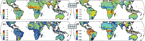
Under the assumption in section 3.1, this work regards ${\epsilon }_{SMAP}^p$ as the reference of surface emissivity, and here mainly discusses the method to generate daily MLSE dataset based on the CYGNSS data. Figure 4 displays the differences in ${\mathrm{\Gamma }}_{\mathit{CYGNSS}}$ and ${\epsilon }_{SMAP}^H$ between January and July and the annual mean values. The correlation between the changes of ${\mathrm{\Gamma }}_{\mathit{CYGNSS}}$ and ${\epsilon }_{SMAP}^H$ is −0.63, and −0.51 for the comparison in yearly averaged values. This indicates a more obvious temporal correlation between ${\mathrm{\Gamma }}_{\mathit{CYGNSS}}$ and ${\epsilon }_{SMAP}^H$ than the spatial correlation. Therefore, inspired by Chew and Small (2018)’s contribution to soil moisture retrieval, a pixel-by-pixel regression algorithm is employed here to model the relationship between ${\mathrm{\Gamma }}_{\mathit{CYGNSS}}$ and ${\epsilon }_{SMAP}^p$, and calculate the CYGNSS emissivity ${\epsilon }_{CYGNSS}^p$ at horizontal and vertical polarization. This pixel-by-pixel algorithm is effective in reducing the impact of intrinsic variability in different areas, such as roughness and soil type, and can significantly improve the accuracy of retrieval (Chen et al. 2022).

Figure 4. The differences in ${\mathrm{\Gamma }}_{\mathit{CYGNSS}}$ and ${\epsilon }_{SMAP}^H$ between January and July and the annual mean values. (a) $\mathrm{\Delta }{\mathrm{\Gamma }}_{\mathit{CYGNSS}}$. (b) $\mathrm{\Delta }{\epsilon }_{SMAP}^H$. (c) ${\mathrm{\Gamma }}_{\mathit{CYGNSS}}$. (d) ${\epsilon }_{SMAP}^H$.

After completing the above calculation, the linear regression is performed independently in each EASE grid cell to derive the model coefficients from the matchups through:

(12) ${\epsilon }_{CYGNSS}^p\left(t_0,\mathit{i}\right)=\mathit{\alpha }\cdot {\mathrm{\Gamma }}_{\mathit{CYGNSS}}\left(t_0,\mathit{i}\right)+\mathit{\beta }\mathit{\hspace{0.17em}}$(12)

where $t_0$ is the day of matchups, $\mathit{\alpha }$ and $\mathit{\beta }$ are the linear coefficients, ${\epsilon }_{CYGNSS}^p$ is the emissivity retrievals from CYGNSS reflectivity. The polarization $\mathit{p}$ is determined by the polarization of the input SMAP brightness temperature. Note that $\mathit{\alpha }$ and $\mathit{\beta }$ vary in each grid cell. Then, the ${\epsilon }_{CYGNSS}^p$ at predicated date $t_1$ can be calculated using the derived coefficients.

To mitigate the risk of overfitting, grid cells with data matchups fewer than 20 are marked as low confidence and excluded from the model training. Furthermore, the use of one-year data for training as well as the limited number of input parameters helped to focus the model on the most relevant information and prevented it from capturing complex, unnecessary patterns that could lead to overfitting.

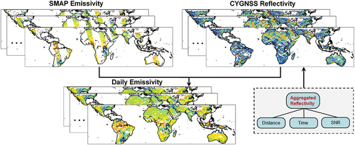
Figure 5 shows the generation process of daily emissivity from CYGNSS reflectivity. The average number of days for collecting SMAP emissivity in all grid cells is 145, and the CYGNSS MLSE has a collection period of 270 days on average. Notably, the temporal resolution of CYGNSS MLSE has significantly improved by 86%, greatly complementing the existing microwave emissivity datasets.

Figure 5. The generation process of daily emissivity from CYGNSS data.

3.4. Outlier removal

The biases in CYGNSS observations and aggregation could bring uncertainties to the retrieval. Thus, an outlier removal method is used here. The “3σ-Hampel identifier” is a more robust filter developed from the well-known “3σ-edit rule”, which can effectively remove the observations with more than three standard deviations from the median (Pearson et al. 2016). The model coefficients are calculated repeatedly until no outliers are generated, and about 7% of observations are removed.

4. Result

4.1. Pan-tropical results

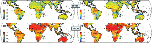
Figure 6 shows the average ${\epsilon }_{CYGNSS}^p$ and ${\epsilon }_{SMAP}^p$ for each grid cell in January 2018. ${\epsilon }_{CYGNSS}^p$ can well reflect the spatial variations in ${\epsilon }_{SMAP}^p$ both in the two polarizations. Overall, a high spatial consistency between them is obtained (R = 0.89 for horizontal polarization emissivity and 0.92 for vertical polarization emissivity, respectively). However, ${\epsilon }_{CYGNSS}^p$ seems to underestimate emissivity in some areas such as the Pampas Steppe and Central Africa.

Figure 6. Comparison of average ${\epsilon }_{CYGNSS}^p$ against average ${\epsilon }_{SMAP}^p$ in January 2018. (a) ${\epsilon }_{CYGNSS}^H$. (b) ${\epsilon }_{SMAP}^H$. (c) ${\epsilon }_{CYGNSS}^V$. (d) ${\epsilon }_{SMAP}^V$.

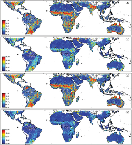
The temporal correlation and root-mean-square error (RMSE) values of ${\epsilon }_{CYGNSS}^p$ against ${\epsilon }_{SMAP}^p$ for each grid cell on the training set are shown in Figure 7. It is clear that the consistency varies across different regions. In certain areas characterized by barren landscapes or dense forests such as the Sahara Desert and the Amazon rainforest, where the variations in emissivity are limited, it is expected to observe low values for both R and RMSE. Conversely, in moderate vegetation areas where emissivity undergoes significant seasonal fluctuations, ${\epsilon }_{CYGNSS}^p$ exhibits a satisfactory correlation with ${\epsilon }_{SMAP}^p$, yielding an RMSE value of around 0.04 for horizontal polarization and around 0.03 for vertical polarization, respectively. Meanwhile, missing results are found in the Tibetan Plateau region, which can be explained by the effect of topographic relief on CYGNSS observation qualities. In addition, due to the systematic difference in the two polarization brightness temperature observations, lower RMSE values are obtained in vertical polarization results.

Figure 7. Statistical indices for ${\epsilon }_{CYGNSS}^p$ against ${\epsilon }_{SMAP}^p$ on the training set. (a) R and (b) RMSE for horizontal polarization emissivity. (c) R and (d) RMSE for vertical polarization emissivity.

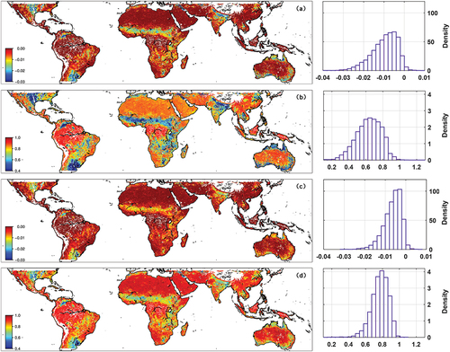
The $\mathit{\alpha }$ values for horizontal polarization emissivity range from −0.021 to 0.001 (5th to 95th percentile, as applicable for all values in this paragraph) and −0.014 to 0.001 for vertical polarization, respectively (Figure 8). On the other hand, the $\mathit{\beta }$ values for horizontal polarization emissivity range from 0.398 to 0.921 and 0.601 to 0.962 for vertical polarization, respectively. It is observed that low $\mathit{\alpha }$ values and high $\mathit{\beta }$ values are predominant in barren landscapes or dense forests, which aligns with the spatial patterns depicted in Figure 7. Near-zero $\mathit{\alpha }$ values typically indicate a low spatial heterogeneity in emissivity. In forested regions, this can be attributed to the interference of microwave signals by dense vegetation, while in arid areas, the lack of soil moisture variability leads to limited fluctuations in emissivity.

Figure 8. Maps and histograms of (a) $\mathit{\alpha }$ values and (b) $\mathit{\beta }$ values for horizontal polarization emissivity, and (c) $\mathit{\alpha }$ values and (b) $\mathit{\beta }$ values for vertical polarization emissivity, respectively. The histograms only include data with R > 0.4.

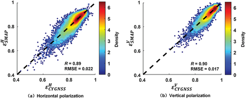
Figure 9 displays the density plot of ${\epsilon }_{CYGNSS}^p$ versus ${\epsilon }_{SMAP}^p$ for all samples on the training set. The dots are well distributed around the 1:1 line and better consistency can be found in dense data. More scattered dots are observed at low emissivity, which is attributed to the high uncertainties in CYGNSS reflectivity under high soil moisture. Specifically, the R and RMSE are 0.89 and 0.022 for horizontal polarization, and 0.90 and 0.017 for vertical polarization, respectively.

Figure 9. Comparisons between ${\epsilon }_{CYGNSS}^p$ and ${\epsilon }_{SMAP}^p$ in the logarithmic scale.

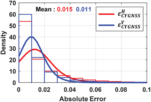
Figure 10 shows the probability density function (PDF) of absolute differences between ${\epsilon }_{CYGNSS}^p$ and ${\epsilon }_{SMAP}^p$ on the training set. More than 75% of ${\epsilon }_{CYGNSS}^H$ have an error of less than 0.02 and the mean error is 0.015, while they are 80% and 0.011 for ${\epsilon }_{CYGNSS}^V$. The proportion of retrievals with high error is small, which indicates the high accuracy and reliability of emissivity retrievals from CYGNSS.

Figure 10. Absolute error PDF of ${\epsilon }_{\mathit{CYGNSS}}$ on the training set.

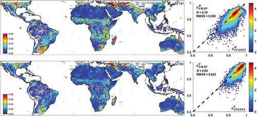
Figure 11 displays the model performance on the test set in terms of temporal RMSE distributions and density plots for both horizontal and vertical polarization, respectively. Good consistency between ${\epsilon }_{CYGNSS}^p$ and ${\epsilon }_{SMAP}^p$ can be seen from this figure. The spatial patterns in RMSE distributions are similar to those observed in the training set results, but significant errors are found in central Madagascar and the northern Arabian Peninsula, which are characterized by plateau terrain. Overall, the R and RMSE are 0.79 and 0.030 for horizontal polarization, and 0.83 and 0.023 for vertical polarization, respectively.

Figure 11. Spatial RMSE distributions and density plots for ${\epsilon }_{CYGNSS}^p$ against ${\epsilon }_{SMAP}^p$ on the test set. (a) Horizontal polarization. (b) Vertical polarization.

To evaluate the performance of ${\epsilon }_{CYGNSS}^p$ in different land types, errors and mean model coefficients are calculated according to the International Geosphere Biosphere Program (IGBP) classes (as shown in Table 1). Classes with a small type percentage are filtered out. The results indicate that accuracy is dependent on the land cover, with the poorest performance observed in croplands due to rapid vegetation growth. Overall, the RMSE for horizontal polarization is consistently below 0.03 for all land types, and below 0.02 for vertical polarization, respectively. As depicted in Figure 8, the spatial patterns align with these findings, where areas characterized by low $\mathit{\alpha }$ values and high $\mathit{\beta }$ values, such as barren areas and dense forests (e.g. Evergreen Broadleaf Forest, Mixed Forests, and Barren or Sparsely Vegetated), exhibit lower errors. These areas tend to display limited variations in emissivity, suggesting that ${\epsilon }_{CYGNSS}^p$ relies more on $\mathit{\beta }$ in these areas rather than the sensitivity of CYGNSS reflectivity to emissivity. However, this also highlights the model’s susceptibility to overfitting in such areas, particularly when emissivity undergoes rapid changes, although such cases are rare.

Table 1. Error statistics and mean model coefficients for different IGBP land types.

Land Type	Percentage (%)	H-polarization				V-polarization
		α	β	RMSE	RMSE (α = 0)	α	β	RMSE	RMSE (α=0)
Evergreen Broadleaf Forest	8.1	−0.0004	0.8857	0.013	0.037	−0.0003	0.9066	0.010	0.026
Deciduous Broadleaf Forest	1.1	−0.0032	0.8091	0.016	0.111	−0.0021	0.8672	0.012	0.070
Mixed Forests	3.5	−0.0008	0.8601	0.014	0.049	−0.0006	0.8908	0.012	0.037
Open Shrublands	18.0	−0.0037	0.7913	0.017	0.148	−0.0025	0.8841	0.013	0.094
Woody Savannas	9.6	−0.0043	0.7512	0.023	0.155	−0.0028	0.8340	0.017	0.102
Savannas	11.5	−0.0068	0.6976	0.025	0.206	−0.0045	0.8065	0.018	0.135
Grasslands	7.3	−0.0093	0.6451	0.026	0.272	−0.0065	0.7743	0.019	0.192
Croplands	10.1	−0.0099	0.6294	0.028	0.257	−0.0066	0.7678	0.020	0.167
Cropland/Natural Vegetation Mosaic	5.2	−0.0062	0.7072	0.024	0.192	−0.0043	0.8044	0.019	0.133
Barren or Sparsely Vegetated	25.3	−0.0008	0.8410	0.011	0.060	−0.0006	0.9293	0.009	0.043
Mean	\	\	\	0.020	0.149	\	\	0.015	0.100

Furthermore, to further analyze the dependence of retrievals on $\mathit{\alpha }$, $\mathit{\alpha }$ values are set to zero for the calculations of ${\epsilon }_{CYGNSS}^p$ and compared with ${\epsilon }_{SMAP}^p$. As shown in Table 1, the mean RMSE values for all land types are 0.020 and 0.015 for horizontal and vertical polarizations, respectively. However, when $\mathit{\alpha }=0$, these values increase to 0.149 and 0.100, respectively. These results demonstrate the significant reliance of ${\epsilon }_{CYGNSS}^p$ on $\mathit{\alpha }$, with a substantial increase in RMSE even in areas where $\mathit{\alpha }$ has low level. It is noteworthy that the retrieval performance in areas with moderate vegetation is more dependent on $\mathit{\alpha }$ compared to other areas, which is consistent with the observed levels of $\mathit{\alpha }$.

4.2. In-situ results

Here, we focus on the results obtained specifically for some ISMN sites. Different from the pan-tropical reference emissivity, the reference here is calculated from SMAP brightness temperature and in-situ temperature records. The CYGNSS data within 0.15° (approximately 14 km) of each site are collected and aggregated using the weight function described in section 3.3 to calculate the effective reflectivity, and the corresponding brightness temperature data are interpolated from the data of the four nearest grid nodes. Figure 12 shows the comparisons between ${\epsilon }_{CYGNSS}^p$ and ${\epsilon }_{SMAP}^p$ for all sites. A good correlation and a low RMSE can be observed for the two polarizations. Similar to pan-tropical results, both ${\epsilon }_{CYGNSS}^H$ and ${\epsilon }_{CYGNSS}^V$ have a better performance at high emissivity, and tend to underestimate at low emissivity. Table 2 lists the RMSE errors for each site. The RMSE ranges from 0.004 to 0.081 for horizontal polarization and 0.005 to 0.076 for vertical polarization, with mean RMSE values of 0.031 and 0.024, respectively.

Figure 12. Comparisons between ${\epsilon }_{CYGNSS}^p$ and ${\epsilon }_{SMAP}^p$ at all in-situ sites.

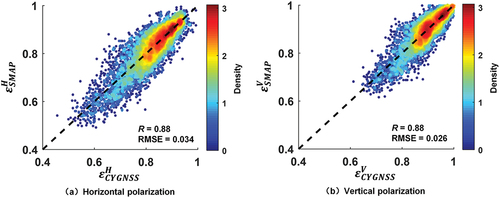
Table 2. Error statistics for all sites.

Site Name	RMSE-H	RMSE-V	Site Name	RMSE-H	RMSE-V	Site Name	RMSE-H	RMSE-V
Anthony	0.036	0.028	MtVernon	0.045	0.039	ElkCabin	0.038	0.023
Ashton	0.047	0.039	NorthIssaquena	0.049	0.017	FORTVALLEY	0.036	0.026
Byron	0.044	0.032	PeeDee	0.016	0.015	HAPPYJACK	0.028	0.022
Lamont	0.047	0.035	PerdidoRivFarms	0.020	0.051	LEECANYON	0.008	0.009
Marshall	0.052	0.040	Perthshire	0.057	0.007	MORMONMTNSUMMIT	0.041	0.030
Morrison	0.059	0.046	PineNut	0.007	0.035	MormonMountain	0.041	0.030
Omega	0.051	0.040	PrairieView#1	0.048	0.033	PALO	0.024	0.019
Pawhuska	0.049	0.041	Princeton#1	0.042	0.036	RAINBOWCANYON	0.009	0.009
Ringwood	0.043	0.033	Riesel	0.051	0.032	SIERRABLANCA	0.077	0.076
Waukomis	0.048	0.039	RiverRoadFarms	0.043	0.036	SenoritaDivide#2	0.043	0.030
AAMU-jtg	0.023	0.017	SanAngelo	0.049	0.012	TresRitos	0.023	0.018
Abrams	0.049	0.038	SandHollow	0.011	0.062	VacasLocas	0.042	0.029
AdamsRanch#1	0.033	0.017	SandyRidge	0.074	0.052	WHITEHORSELAKE	0.033	0.027
Alcalde	0.017	0.017	Scott	0.062	0.017	Asheville-13-S	0.012	0.009
AllenFarms	0.027	0.021	Selma	0.022	0.042	Batesville-8-WNW	0.036	0.028
Beaumont	0.029	0.024	SilverCity	0.049	0.021	Bowling-Green-21-NNE	0.040	0.032
BraggFarm	0.027	0.021	StanleyFarm	0.027	0.024	Bronte-11-NNE	0.048	0.034
Bushland#1	0.039	0.023	Starkville	0.031	0.027	Cortez-8-SE	0.027	0.016
Charkiln	0.008	0.007	Stephenville	0.037	0.008	Durham-11-W	0.021	0.018
CochoraRanch	0.031	0.020	Stubblefield	0.006	0.020	Edinburg-17-NNE	0.011	0.019
DesertCenter	0.004	0.005	SudduthFarms	0.027	0.018	Elgin-5-S	0.007	0.008
Dexter	0.061	0.050	TidewaterArec	0.021	0.009	Gadsden-19-N	0.030	0.024
EastviewFarm	0.023	0.018	TroughSprings	0.007	0.068	Goodwell-2-E	0.034	0.020
Essex	0.005	0.005	Tunica	0.081	0.017	Goodwell-2-SE	0.032	0.019
EvergladesArs	0.044	0.037	Tuskegee	0.021	0.013	Holly-Springs-4-N	0.029	0.024
FordDryLake	0.007	0.007	TwinPinesConservationArea	0.016	0.052	Lafayette-13-SE	0.047	0.039
FortReno#1	0.037	0.026	UAPBDewitt	0.061	0.031	Las-Cruces-20-N	0.009	0.008
GoodwinCreekTimber	0.044	0.033	UAPBLonokeFarm	0.040	0.042	Merced-23-WSW	0.059	0.042
Hodges	0.030	0.024	UAPBMarianna	0.051	0.027	Mercury-3-SSW	0.007	0.006
IsbellFarms	0.025	0.019	UAPBPointRemove	0.034	0.025	Monahans-6-ENE	0.006	0.011
JornadaExpRange	0.007	0.007	Uvalde	0.034	0.020	Monroe-26-N	0.041	0.033
JournaganRanch	0.035	0.025	Vernon	0.033	0.028	Muleshoe-19-S	0.024	0.012
KoptisFarms	0.021	0.016	WTARS	0.042	0.025	Newton-11-SW	0.028	0.020
KyleCanyon	0.008	0.010	Vermillion	0.033	0.012	Newton-5-ENE	0.017	0.014
Levelland	0.026	0.014	Wakulla#1	0.012	0.019	Newton-8-W	0.031	0.022
LittleRiver	0.034	0.024	WalnutGulch#1	0.031	0.014	Panther-Junction-2-N	0.026	0.019
Livingston-UWA	0.022	0.017	Watkinsville#1	0.017	0.013	Socorro-20-N	0.006	0.006
LosLunasPmc	0.012	0.010	Weslaco	0.029	0.013	Stillwater-2-W	0.045	0.033
LovellSummit	0.010	0.013	YoumansFarm	0.017	0.026	Stillwater-5-WNW	0.048	0.036
MammothCave	0.040	0.032	BAKERBUTTESMT	0.032	0.007	Stovepipe-Wells-1-SW	0.008	0.008
Mayday	0.028	0.024	BRISTLECONETRAIL	0.009	0.029	Tucson-11-W	0.009	0.009
McalisterFarm	0.031	0.023	BakerButte	0.035	0.022	Watkinsville-5-SSE	0.022	0.017
MonoclineRidge	0.007	0.008	BarM	0.032	0.021	Williams-35-NNW	0.042	0.025
MorrisFarms	0.025	0.020	Chalender	0.026	0.039	Yuma	0.007	0.006
				Mean	RMSE-H : 0.031 RMSE-V : 0.024

To further assess the accuracy of CYGNSS-retrieved emissivity compared with in-situ measurements, the time series and emissivity comparisons of six sites are displayed in Figure 13. The sites are representatively selected from the Atmospheric Radiation Measurement (ARM), Soil Climate Analysis Network (SCAN), and U.S. Climate Reference Network (USCRN), where MLSE values exhibit ample variations. Limited in space, only results of horizontal polarization are shown here. The gray lines represent the ${\epsilon }_{CYGNSS}^H$ both at matched date and the predicted date, while the blue dots represent the reference ${\epsilon }_{SMAP}^H$. The time-series plots manifest the satisfactory consistency between ${\epsilon }_{CYGNSS}^H$ and ${\epsilon }_{SMAP}^H$, especially on the days with drastic variations. The R values for the six sites range from 0.65 to 0.88, and the RMSE ranges from 0.022 to 0.048, respectively. Additionally, it is evident that CYGNSS can effectively provide daily emissivity estimations. The average number of days for collecting SMAP emissivity at these sites is 143, whereas the number for aggregated CYGNSS reflectivity is 311. Studies have proved that soil moisture is a key factor affecting emissivity. However, it is clear from the figure that the peaks of ${\epsilon }_{SMAP}^H$ and soil moisture do not always correspond one-to-one. This indicates emissivity is a complex parameter affected by many factors such as soil moisture, vegetation structure, and biomass. Thus, the CYGNSS derived reflectivity, which is also produced under the influence of the same environmental factors, can be a suitable alternative to MLSE for microwave remote sensing.

Figure 13. Time series (left) and error statistics (right) of ${\epsilon }_{CYGNSS}^H$ versus ${\epsilon }_{SMAP}^H$ at six sites: Waukomis [36.33N, 97.89W], AAMU-jtg [34.78N, 86.59W], Levelland [33.59N, 102.37W], Starkville [33.67N, 88.74W], Goodwell-2-SE [36.59N, 101.62W], and Newton-8-W [31.34N, 84.45W]. The blue dots refer to ${\epsilon }_{SMAP}^H$, the gray lines refer to ${\epsilon }_{CYGNSS}^H$, and the green bars refer to soil moisture.

5. Conclusions

This study presents and evaluates a method for estimating daily MLSE in the pan-tropical region using GNSS-R data. The proposed method uses a combined weight function of distance, time, and SNR variance to aggregate CYGNSS observations into the EASE 2.0 36 km grid, and employs a pixel-by-pixel regression algorithm to retrieve daily MLSE. The CYGNSS MLSE exhibits good agreement with SMAP brightness temperature derived MLSE, with an overall RMSE of 0.022 and 0.017 for horizontal and vertical polarization on the training set, and an RMSE of 0.030 and 0.023 on the test set, respectively. ISMN temperature records are utilized for in-situ validation, and both show good consistency with an RMSE of 0.034 and 0.026 for horizontal and vertical polarization, respectively. The accuracy of CYGNSS MLSE depends on the land cover, with errors obtained in dense vegetation and barren areas being significantly less than in other areas. Additionally, the temporal resolution of CYGNSS MLSE shows a remarkable improvement of 86% compared to SMAP MLSE, which can greatly complement the microwave emissivity dataset at the daily scale.

The satisfactory CYGNSS MLSE demonstrates an encouraging approach to obtain a daily MLSE dataset for microwave remote sensing. When compared to SMAP sensors, CYGNSS has an obvious advantage in terms of spatial and temporal resolution. In this work, CYGNSS data are aggregated in the EASE grid to allow for spatial comparison with SMAP data. Once the physical model for transforming the GNSS reflectometer to microwave radiometry is developed, it is expected that CYGNSS emissivity can be independently calculated with higher spatial and temporal resolution, without the need for SMAP data as a reference. Furthermore, it is worth noting that most existing emissivity studies only focus on clear-sky conditions, while this study retrieves MLSE under all weather conditions.

Disclosure statement

No potential conflict of interest was reported by the author(s).

Data availability statement

The CYGNSS data are openly available at https://podaac.jpl.nasa.gov., the SMAP data are available at https://smap.jpl.nasa.gov/data/., the ISMN data are available at https://ismn.earth/en/., and the GSW data are available at https://global-surface-water.appspot.com/.

Additional information

Funding

This work was supported by the National Natural Science Foundation of China [grant number 42074029], the Natural Science Foundation of Hubei Province for Distinguished Young Scholars [grant number 2021CFA039], and the Fundamental Research Funds for the Central Universities [grant number 2042023kfyq01].

Notes on contributors

Yifan Zhu

Yifan Zhu is currently a PhD candidate at Wuhan University. He obtained his M.Sc. degree from Nanjing Normal University in 2021. His current research focuses on GNSS-R.

Fei Guo

Fei Guo is currently a professor at Wuhan University. He obtained his M.Sc. and PhD degrees with distinction in geodesy from Wuhan University in 2009 and 2013, respectively. His current research mainly focuses on GNSS-R and precise GNSS positioning.

Xiaohong Zhang

Xiaohong Zhang is currently a professor at Wuhan University. He obtained his M.Sc. and Ph.D. degrees with distinction in geodesy and engineering surveying at Wuhan University in 1999 and 2002, respectively. His main research interests include PPP, GNSS/INS navigation, and their applications in geoscience and engineering.

Wentao Yang

Wentao Yang is currently a PhD candidate at Wuhan University. He received the MS degree from Chang’an University in 2022. His research interests are in Global Navigation Satellite System (GNSS) remote sensing.

References

- Alonso-Arroyo, A., V. U. Zavorotny, and A. Camps. 2017. “Sea Ice Detection Using UK TDS-1 GNSS-R Data.” IEEE Transactions on Geoscience and Remote Sensing 55 (9): 4989–5001. https://doi.org/10.1109/TGRS.2017.2699122.
- Campbell, J. D., R. Akbar, A. Bringer, D. Comite, L. Dente, S. T. Gleason, L. Guerriero, E. Hodges, J. T. Johnson, and S. Kim. 2022. “Intercomparison of Electromagnetic Scattering Models for Delay-Doppler Maps Along a CYGNSS Land Track with Topography.” IEEE Transactions on Geoscience and Remote Sensing 60:1–13. https://doi.org/10.1109/TGRS.2022.3210160.
- Camps, A., H. Park, M. Pablos, G. Foti, C. P. Gommenginger, P. Liu, and J. Judge. 2016. “Sensitivity of GNSS-R Spaceborne Observations to Soil Moisture and Vegetation.” IEEE Journal of Selected Topics in Applied Earth Observations and Remote Sensing 9 (10): 4730–4742. https://doi.org/10.1109/JSTARS.2016.2588467.
- Chan, S., E. G. Njoku, and A. Colliander. 2020. SMAP L1C Radiometer Half-Orbit 36 Km EASE-Grid Brightness Temperatures, Version 5 [Data Set]. Boulder, Colorado USA: NASA National Snow and Ice Data Center Distributed Active Archive Center. Accessed December 1, 2024. https://doi.org/10.5067/JJ5FL7FRLKJI.
- Chen, F., X. Zhang, F. Guo, J. Zheng, Y. Nan, and M. Freeshah. 2022. “TDS-1 GNSS Reflectometry Wind Geophysical Model Function Response to GPS Block Types.” Geo-Spatial Information Science 25 (2): 312–324. https://doi.org/10.1080/10095020.2021.1997076.
- Chen, S., Q. Yan, S. Jin, W. Huang, T. Chen, Y. Jia, S. Liu, and Q. Cao. 2022. “Soil Moisture Retrieval from the CyGNSS Data Based on a Bilinear Regression.” Remote Sensing 14 (9): 1961. https://doi.org/10.3390/rs14091961.
- Chew, C. C., and E. E. Small. 2018. “Soil Moisture Sensing Using Spaceborne GNSS Reflections: Comparison of CYGNSS Reflectivity to SMAP Soil Moisture.” Geophysical Research Letters 45 (9): 4049–4057. https://doi.org/10.1029/2018GL077905.
- Chew, C., and E. Small. 2020. “Description of the UCAR/CU Soil Moisture Product.” Remote Sensing 12 (10): 1558. https://doi.org/10.3390/rs12101558.
- Clarizia, M. P., N. Pierdicca, F. Costantini, and N. Floury. 2019. “Analysis of CYGNSS Data for Soil Moisture Retrieval.” IEEE Journal of Selected Topics in Applied Earth Observations and Remote Sensing 12 (7): 2227–2235. https://doi.org/10.1109/JSTARS.2019.2895510.
- Cygnss. 2017. Cygnss Level 1 Science Data Record Version 2.1. Edited: NASA Physical Oceanography Distributed Active Archive Center. https://doi.org/10.5067/CYGNS-L1X21.
- Dong, Z., and S. Jin. 2021. “Evaluation of the Land GNSS-Reflected DDM Coherence on Soil Moisture Estimation from CYGNSS Data.” Remote Sensing 13 (4): 570. https://doi.org/10.3390/rs13040570.
- Dorigo, W. A., W. Wagner, R. Hohensinn, S. Hahn, C. Paulik, A. Xaver, A. Gruber, et al. 2011. “The International Soil Moisture Network: A Data Hosting Facility for Global in situ Soil Moisture Measurements.” Hydrology and Earth System Sciences 15 (5): 1675–1698. https://doi.org/10.5194/hess-15-1675-2011.
- Entekhabi, D., E. G. Njoku, P. E. O’Neill, K. H. Kellogg, W. T. Crow, W. N. Edelstein, J. K. Entin, et al. 2010. “The Soil Moisture Active Passive (SMAP) Mission.” Proceedings of the IEEE 98 (5): 704–716. https://doi.org/10.1109/JPROC.2010.2043918.
- Entekhabi, D., S. Yueh, P. E. O’Neill, K. H. Kellogg, A. Allen, R. Bindlish, M. Brown, S. Chan, A. Colliander, W. T. Crow, et al. 2010. “SMAP Handbook: Soil Moisture Active Passive: Mapping Soil Moisture and Freeze/Thaw from Space; Jet Propulsion Laboratory, California Institute of Technology: Pasadena, CA, USA.” Accessed January 8, 2020. https://smap.jpl.nasa.gov/system/internal_resources/details/original/178_SMAP_Handbook_FINAL_1_JULY_2014_Web.pdf.
- Eroglu, O., M. Kurum, D. Boyd, and A. C. Gurbuz. 2019. “High Spatio-Temporal Resolution CYGNSS Soil Moisture Estimates Using Artificial Neural Networks.” Remote Sensing 11 (19): 2272. https://doi.org/10.3390/rs11192272.
- Gleason, S., C. S. Ruf, A. J. O’Brien, and D. S. Mckague. 2018. “The CYGNSS Level 1 Calibration Algorithm and Error Analysis Based on On-Orbit Measurements.” IEEE Journal of Selected Topics in Applied Earth Observations and Remote Sensing 12 (1): 37–49. https://doi.org/10.1109/JSTARS.2018.2832981.
- Jackson, T. J., and T. J. Schmugge. 1991. “Vegetation Effects on the Microwave Emission of Soils.” Remote Sensing of Environment 36 (3): 203–212. https://doi.org/10.1016/0034-4257(91)90057-D.
- Jin, S., Q. Wang, and G. Dardanelli. 2022. “A Review on Multi-GNSS for Earth Observation and Emerging Applications.” Remote Sensing 14 (16): 3930. https://doi.org/10.3390/rs14163930.
- Jing, C., W. Li, W. Wan, F. Lu, X. Niu, X. Chen, A. Rius, et al. 2024. “A Review of the BuFeng-1 GNSS-R Mission: Calibration and Validation Results of Sea Surface and Land Surface.” Geo-Spatial Information Science: 1–15. https://doi.org/10.1080/10095020.2024.2330547.
- Karbou, F., C. Prigent, L. Eymard, and J. R. Pardo. 2005. “Microwave Land Emissivity Calculations Using AMSU Measurements.” IEEE Transactions on Geoscience and Remote Sensing 43 (5): 948–959. https://doi.org/10.1109/TGRS.2004.837503.
- Li, Z., F. Guo, F. Chen, Z. Zhang, and X. Zhang. 2023. “Wind Speed Retrieval Using GNSS-R Technique with Geographic Partitioning.” Satellite Navigation 4 (1): 4. https://doi.org/10.1186/s43020-022-00093-z.
- Min, Q., B. Lin, and R. Li. 2009. “Remote Sensing Vegetation Hydrological States Using Passive Microwave Measurements.” IEEE Journal of Selected Topics in Applied Earth Observations and Remote Sensing 3 (1): 124–131. https://doi.org/10.1109/JSTARS.2009.2032557.
- Moncet, J., P. Liang, J. F. Galantowicz, A. E. Lipton, G. Uymin, C. Prigent, and C. Grassotti. 2011. “Land Surface Microwave Emissivities Derived from AMSR-E and MODIS Measurements with Advanced Quality Control.” Journal of Geophysical Research: Atmospheres 116 (D16): 116. https://doi.org/10.1029/2010JD015429.
- Norouzi, H., M. Temimi, W. B. Rossow, C. Pearl, M. Azarderakhsh, and R. Khanbilvardi. 2011. “The Sensitivity of Land Emissivity Estimates from AMSR-E at C and X Bands to Surface Properties.” Hydrology and Earth System Sciences 15 (11): 3577–3589. https://doi.org/10.5194/hess-15-3577-2011.
- O’Neill, P. E., S. Chan, E. G. Njoku, T. Jackson, R. Bindlish, and J. Chaubell. 2020. SMAP L3 Radiometer Global Daily 36 Km EASE-Grid Soil Moisture, Version 7. Boulder, Colorado USA: NASA National Snow and Ice Data Center Distributed Active Archive Center. Accessed November 1, 2024. https://doi.org/10.5067/HH4SZ2PXSP6A.
- Pearson, R. K., Y. Neuvo, J. Astola, and M. Gabbouj. 2016. “Generalized Hampel Filters.” Eurasip Journal on Advances in Signal Processing 2016 (1): 87. https://doi.org/10.1186/s13634-016-0383-6.
- Pekel, J., A. Cottam, N. Gorelick, and A. S. Belward. 2016. “High-Resolution Mapping of Global Surface Water and its Long-Term Changes.” Nature 540 (7633): 418–422. https://doi.org/10.1038/nature20584.
- Prigent, C., W. B. Rossow, and E. Matthews. 1997. “Microwave Land Surface Emissivities Estimated from SSM/I Observations.” Journal of Geophysical Research: Atmospheres 102 (D18): 21867–21890. https://doi.org/10.1029/97JD01360.
- Ringerud, S., C. Kummerow, and C. Peters-Lidard. 2015. “A Semi-Empirical Model for Computing Land Surface Emissivity in the Microwave Region.” IEEE Transactions on Geoscience & Remote Sensing 53 (4): 1935–1946. https://doi.org/10.1109/TGRS.2014.2351232.
- Ringerud, S., C. Kummerow, C. Peters-Lidard, Y. Tian, and K. Harrison. 2013. “A Comparison of Microwave Window Channel Retrieved and Forward-Modeled Emissivities Over the U.S. Southern Great Plains.” IEEE Transactions on Geoscience & Remote Sensing 52 (5): 2395–2412. https://doi.org/10.1109/TGRS.2013.2260759.
- Ruf, C. S., R. Atlas, P. S. Chang, M. P. Clarizia, J. L. Garrison, S. Gleason, S. J. Katzberg, et al. 2016. “New Ocean Winds Satellite Mission to Probe Hurricanes and Tropical Convection.” Bulletin of the American Meteorological Society 97 (3): 385–395. https://doi.org/10.1175/BAMS-D-14-00218.1.
- Saïd, F., Z. Jelenak, J. Park, and P. S. Chang. 2021. “The NOAA Track-Wise Wind Retrieval Algorithm and Product Assessment for CyGNSS.” IEEE Transactions on Geoscience and Remote Sensing 60:1–24. https://doi.org/10.1109/TGRS.2021.3087426.
- Tian, Y., C. D. Peters Lidard, K. W. Harrison, Y. You, S. Ringerud, S. Kumar, and F. J. Turk. 2015. “An Examination of Methods for Estimating Land Surface Microwave Emissivity.” Journal of Geophysical Research Atmospheres 120 (21): 111–114, 128. https://doi.org/10.1002/2015JD023582.
- Turk, F. J., Z. S. Haddad, and Y. You. 2014. “Principal Components of Multifrequency Microwave Land Surface Emissivities. Part I: Estimation Under Clear and Precipitating Conditions.” Journal of Hydrometeorology 15 (1): 3–19. https://doi.org/10.1175/JHM-D-13-08.1.
- Weng, F., B. Yan, and N. C. Grody. 2001. “A Microwave Land Emissivity Model.” Journal of Geophysical Research: Atmospheres 106 (D17): 20115–20123. https://doi.org/10.1029/2001JD900019.
- Wu, Y., J. Bao, Z. Liu, Y. Bao, and G. P. Petropoulos. 2022. “Investigation of the Sensitivity of Microwave Land Surface Emissivity to Soil Texture in MLEM.” Remote Sensing 14 (13): 3045. https://doi.org/10.3390/rs14133045.
- Yan, Q., W. Huang, S. Jin, and Y. Jia. 2020. “Pan-Tropical Soil Moisture Mapping Based on a Three-Layer Model from CYGNSS GNSS-R Data.” Remote Sensing of Environment 247:111944. https://doi.org/10.1016/j.rse.2020.111944.
- Yang, T., W. Wan, J. Wang, B. Liu, and Z. Sun. 2022. “A Physics-Based Algorithm to Couple CYGNSS Surface Reflectivity and SMAP Brightness Temperature Estimates for Accurate Soil Moisture Retrieval.” IEEE Transactions on Geoscience and Remote Sensing 60:1–15. https://doi.org/10.1109/TGRS.2022.3156959.
- Yang, W., F. Guo, X. Zhang, and Y. Zhu. 2023. “An Improved Method for Water Body Removal in Spaceborne GNSS-R Soil Moisture Retrieval.” IEEE Transactions on Geoscience and Remote Sensing 61:1–8. https://doi.org/10.1109/TGRS.2023.3264629.
- Zhang, J., T. Zhao, S. Tan, N. Rodriguez-Fernandez, H. Xue, N. Yang, Y. Kerr, and J. Shi. 2023. “Characterizing the Channel Dependence of Vegetation Effects on Microwave Emissions from Soils.” Geo-Spatial Information Science 1–17. https://doi.org/10.1080/10095020.2023.2275616.
- Zribi, M., D. Guyon, E. Motte, S. Dayau, J. P. Wigneron, N. Baghdadi, and N. Pierdicca. 2019. “Performance of GNSS-R GLORI Data for Biomass Estimation Over the Landes Forest.” International Journal of Applied Earth Observation and Geoinformation 74:150–158. https://doi.org/10.1016/j.jag.2018.09.010.