A multi-scale attributes fusion model for travel mode identification using GPS trajectories

ABSTRACT

Travel mode recognition is a key issue in urban planning and transportation research. While traditional travel surveys use manual data collection and have limited coverage, poor timeliness, and insufficient sample capacity, recent advancements in Global Positioning System (GPS) technology allow large-scale data collection and offer novel opportunities to enhance travel mode recognition. However, existing studies often neglect regular differences and changes in motion states across different travel modes and fail to fully integrate multi-scale spatio-temporal features, which limits the accurate classification of travel modes. To fill this gap, this study proposes a multi-scale spatio-temporal attribute fusion (MSAF) model for precise travel mode identification using solely GPS trajectories without altering their sampling rate. The MSAF model segments GPS trajectories into various temporal and spatial scales, extracting local motion states and spatial features at multiple scales. The spatio-temporal feature extraction module is constructed to extract local motion states and capture spatio-temporal dependencies. Additionally, the model incorporates a multi-scale feature fusion module, which effectively combines features of various scales through a series of fusion techniques to obtain a comprehensive representation, enabling automatic and accurate travel mode identification. Experiments on real-world datasets, including the GeoLife Trajectories dataset and the Sussex-Huawei Locomotion-Transportation (SHL) dataset, demonstrate the effectiveness of the MSAF model, achieving a competitive accuracy of 95.16% and 91.70%. This represents an improvement of 2.50% to 7.95% and 0.8% to 6.62% over several state-of-the-art baselines, effectively addressing sample imbalance challenges. Moreover, the experiments demonstrate the significant role of multiscale feature fusion in improving model performance.

KEYWORDS:

• GPS trajectory
• travel mode identification
• trajectory segmentation
• multi-scale attributes
• spatio-temporal convolution

1. Introduction

Accurate travel mode identification (TMI) is crucial for urban transportation planning and pollution management (James 2020; Ju, Zeng, and Zhang 2024). Understanding travel demand and residents’ spatial distribution allows the transportation sector to develop appropriate measures and optimize resource allocation to mitigate travel-related issues, including increased travel time, traffic congestion, and air pollution (Zhang et al. 2024). Traditional travel mode surveys gather information through phone calls and interviews, a method constrained by cost, scope, and accuracy limitations that ultimately reduce data quality (Sadeghian, Håkansson, and Zhao 2021). Positioning data collected through GPS has recently enabled the rapid identification of residents’ commuting patterns (Yang et al. 2018).

Existing studies address this challenge through a three-step process: trajectory segmentation (Zhu et al. 2021), feature construction (Xiao et al. 2017), and mode recognition (Wang et al. 2020). Trajectory segmentation divides a continuous path into discrete segments to capture abundant feature data (Dabiri et al. 2019). However, existing studies predominantly use equalization methods, neglecting each travel mode’s regularity and motion status changes, resulting in deviations between extracted eigenvalues and actual values. Feature construction involves extracting attributes that represent the motion state (e.g. velocity, distance, and direction) and then converting them into a fixed feature structure (e.g. a vector, feature matrix, single-channel sequence, multi-channel sequence, or image) for input into a downstream model (Zhang et al. 2021). Travel pattern recognition is then implemented through rule-based and learning-based approaches. However, rule-based approaches rely heavily on the researcher’s prior knowledge and personal experience (Zan et al. 2023). Traditional machine learning algorithms, in contrast, typically extract only shallow features with non-linear variations, which limits their ability to extract features for non-linear and complex trajectory data. This limitation makes capturing subtle differences and correlations among various travel modes challenging. These methods are also limited when dealing with large-scale trajectory data and complex travel scenarios (Nawaz et al. 2020). To address these constraints, the proposed transportation mode recognition field increasingly incorporates deep learning techniques (Dabiri et al. 2020). Through powerful feature learning and nonlinear mapping capabilities, this approach effectively captures complex spatio-temporal relationships (Jiang et al. 2023) in trajectory data, further enhancing the accuracy of travel mode identification. A fixed input size usually causes these methods to ignore both the spatio-temporal heterogeneity among different moving trajectories and the influence of feature scale on the recognition results, so they fail to fully extract the multiscale spatio-temporal features of the trajectory motion state. To effectively capture the spatial and temporal differences in trajectory features, this study uses dynamic multi-scale segmentation of travel trajectories and explores the effect of multi-scale feature fusion modules on travel mode recognition.

This study proposes a multi-scale spatio-temporal attribute fusion (MSAF) model to overcome such restrictions through accurate TMI using GPS trajectories. The key contributions of this study are summarized as follows:

1. A novel dynamic segmentation method for trajectories is introduced to more accurately capture the distinct properties of various transportation modes. This method integrates temporal and spatial information and uses an adaptive segmentation strategy. The approach effectively identifies distinct parts with similar motion states by dynamically selecting and dividing segments based on the trajectory’s spatio-temporal characteristics. Kinematic and geometric properties are then extracted at various scales from each segment, allowing a more accurate and comprehensive capture of kinematic changes in the trajectory data.

2. For accurate end-to-end travel mode identification, the MSAF model is proposed. The model first fuses local motion states and captures embedded spatio-temporal dependencies through channel-level concatenation of multi-scale feature matrices. Then, feature information is combined with varying weights and spatio-temporal scales to enhance the characterization of spatio-temporal features. Finally, a fully connected neural network layer integrates the features at each scale to produce the ultimate recognition results for travel modes.

3. Extensive experiments are conducted on publicly available datasets, GeoLife and SHL (Gjoreski et al. 2018; Wang et al. 2019), to evaluate the proposed MSAF model’s effectiveness. The results achieve an accuracy of 95.16% and 91.70% and exhibit an average accuracy improvement ranging from 2.50–7.95% to 0.80–6.62%, demonstrating the model’s effectiveness and the method’s ability to compete with several state-of-the-art baselines. These experimental results validate the significant role of multi-scale feature fusion in enhancing model performance.

The paper’s structure is as follows: Section 2 reviews existing research on trajectory feature extraction and pattern recognition methods. Section 3 defines the relevant concepts of trajectory features, such as speed, acceleration, direction, and curvature. Section 4 details the proposed MSAF framework’s data processing, feature extraction, model structure, and result evaluation. Section 5 introduces the GeoLife and SHL datasets, followed by a discussion of the implementation details and experiment results. The conclusions are then summarized in Section 6.

2. Related works

For 15 years, TMI has been defined as a classification task. The process of identifying travel modes follows a structured approach. First, GPS data undergo segmentation based on established guidelines, converting GPS data points into trajectory segments. Motion parameters relevant to these trajectory segments and GPS sampling point attributes are then calculated. These parameters create a feature set fed into the downstream model to recognize and classify travel modes. This section reviews related work concerning trajectory segmentation, feature engineering, and recognition methods based on the imperative steps of travel pattern recognition.

2.1. Trajectory segmentation

Trajectory segmentation is a vital aspect of feature engineering (Guo et al. 2020; Kim, Kim, and Lee 2022; Xiao, Cheng, and Zhang 2019) and is classified into two categories: number of samples-based and sampling time-based methods, depending on the attributes utilized. The method based on the number of sampling points homogenizes the trajectory into multiple segments with an equal number of sampling points to capture changing characteristics at different moments and locations (Dabiri and Heaslip 2018). Due to the temporal heterogeneity in GPS trajectory collection and the uneven temporal and spatial distribution of segments, capturing the trajectory characteristics of various travel modes is challenging (Li et al. 2020). One strategy to reduce the sampling frequency impact is to resample the trajectory to obtain consistent data and then segment it into fixed time intervals (Jiang et al. 2020). However, this method can only extract features at a fixed scale and overlooks differences in motion states for trajectories of various transportation modes. The motion states of various traveling modes are intricate. For instance, buses and subways may remain stationary while stopping at a station, and a fixed-scale segmentation method could yield smaller eigenvalues for the trajectory segment than actual values. Therefore, to enhance trajectory segmentation and feature extraction accuracy, it is crucial to develop dynamic segmentation rules that can better adapt to the trajectory features of various travel modes.

2.2. Feature engineering

Feature engineering in trajectory analysis involves extracting motion, temporal, and spatial features from trajectory points and segments. These features are subsequently integrated into predefined structures for input into downstream recognition models, allowing efficient analysis and recognition of trajectory data.

2.2.1. Feature extraction

The process of trajectory feature extraction involves obtaining quantitative descriptions of motion patterns, spatio-temporal relationships, and related information from GPS trajectory data. These features include motion, geometric attributes, frequency domain characteristics, and additional relevant parameters as shown in Table 1. Motion features are derived from changes in attributes (e.g. time, longitude, and latitude between successive trajectory points) that provide insight into the movement dynamics. Geometric features focus on the spatial shape and structure of the trajectory path (e.g. deflection angle and curvature) to characterize the trajectory’s geometric properties. Frequency domain features analyze a trajectory’s regularity and vibratory pattern from a frequency perspective, revealing underlying patterns in the data. Other studies incorporate supplementary trajectory data features (e.g. land use type, date, travel time, and environmental traffic conditions) to enrich the feature set and enhance the trajectory analysis accuracy.

Table 1. Classification of trajectory characteristics.

Class	General features
Motion features	Average speed, acceleration, maximum speed, minimum speed, etc;
Geometric features	Deflection angle, distance, curvature, etc;
Frequency domain feature	Periodicity, frequency distribution, spectral energy, frequency peaks, etc;
Other features	Land use, POI, road type, age, gender, weather conditions, weekdays, etc.

2.2.2. Feature construction

The structure of trajectory features can be categorized into five main types according to division methods and forms: vectors, one-dimensional multi-channel sequences, feature matrices, multi-dimensional multi-channel sequences, and images. Figure 1 summarizes the various types of trajectory features.

Figure 1. Summary of trajectory feature structures.

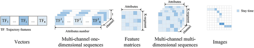
Early studies treated trajectory data as a unified entity, converting it into numerical vectors to capture overarching attributes (e.g. mean velocity, distance, and curvature). Multi-channel one-dimensional sequences, an extension of feature vectors, introduced multiple channels to represent diverse features. While this allowed for more detailed extraction of global feature attributes (e.g. maximum, minimum, and variance), such methods were confined to conventional machine learning techniques like Support Vector Machines (SVM) and Random Forests (RF). When faced with intricate trajectory data from various travel modes, these essential feature structures struggle to effectively capture the inherent motion characteristics. In this study, the feature structures adopt a more thorough approach by segmenting and modeling the trajectory data. Consequently, the feature matrix transforms the trajectory data into a matrix format, with rows and columns representing trajectory segments and feature attributes. Multi-channel multi-dimensional sequences are then employed to comprehensively represent various feature attributes, both global and local, by introducing multiple channels. Trajectory data is then mapped onto an image grid, with the grid size determined by the trajectory data sampling time. This structure, commonly used in deep learning models, assists the process of extracting spatial and temporal characteristics by utilizing techniques like convolutional and recurrent neural networks to create more sophisticated feature representations. Several additional studies exclusively segmented trajectories at a fixed scale, overlooking the diversity of travel modes and the impact of multi-scale feature fusion on travel mode identification.

2.3. Pattern recognition methods

Existing models for recognizing traffic modes are classified into rule-based, probability-based, and machine-learning methods.

2.3.1. Rule-based approach

Rule-based methods manually create rules to perform feature extraction and travel mode recognition using trajectory data (Shen and Stopher 2014). Trajectory classification is primarily achieved by establishing rules and thresholds related to travel speed, time, acceleration, and deceleration. For example, the rules delineate (a) walking speeds below 6 km/h (Stopher, Jiang, and FitzGerald 2005) and (b) car speeds above 30 km/h (Yamada et al. 2016). Researchers (Hui et al. 2017) have also employed two straightforward guidelines to deduce travel patterns between Canadian cities by (a) opting for air travel if the travel time is 0.5–1.5 h and (b) choosing surface travel if the travel time is 2–6 h. In some cases, acceleration and deceleration are used to differentiate between modes of travel, such as walking, bicycling, transit, and automobile (Stopher et al. 2008).

While rule-based methods offer speedy execution, they heavily depend on the researcher’s prior knowledge and personal experience for setting recognition rules and thresholds. This dependence challenges the distinction between travel modes with similar movement characteristics (e.g. bicycles and buses). Rule-based approaches do not fully capitalize on large-scale data and complex feature engineering, limiting their potential to address the more complex and diverse challenges associated with identifying travel modes.

2.3.2. Probability-based approaches

The probability-based approach involves predicting the likelihood of each transportation mode using GPS data and survey details. The method compares thresholds and probabilities, identifying the transportation mode with the highest probability as the estimated outcome (Gong et al. 2014). For example, a fuzzy logic rule approach distinguishes between four modes of travel: car, transit, cycling, and walking (Tsui and Shalaby 2006). Researchers analyzed GPS data from 237 track segments collected by nine volunteers, extracting features such as average speed, 95th percentile maximum speed, forward median acceleration, and GPS track segment data quality. By employing a fuzzy inference system and affiliation function parameter, likelihood scores for different travel modes were derived, which permitted the recognition of the travel modes of the track segments. Another study used a probability matrix-based method to assess the likelihood of each transportation mode based on criteria, such as average speed, maximum speed, speed distribution, and distance traveled. Using GPS location information, the probability matrix was subsequently utilized to recognize the five transportation modes (Stopher et al. 2008). For instance, walking modes with a high likelihood exhibit an average speed of less than 6 km/h and a maximum speed of less than 10 km/h. The final scores for walking, cycling, and driving were calculated by combining the probabilities of each transportation mode, and further differentiation between cars and buses was achieved through transportation network layers. Despite achieving up to 95% accuracy in transportation mode identification, limitations persist due to the model’s excessive reliance on a single speed variable, inconsistent GPS recordings, and potential misclassification risks during the final stage when utilizing the traffic layer.

2.3.3. Machine learning methods

Machine learning approaches facilitate the classification and automatic identification of travel modes by extracting and categorizing trajectory data using two primary methodologies: unsupervised and supervised.

The unsupervised approach categorizes trajectory data based on trajectory features, employing classical methods such as KNN, DBSCAN, and hierarchical clustering. For instance, clustering trajectory speeds permit the recognition of walking, bus, and car modes with 84% accuracy (Patterson et al. 2003). However, the study’s dataset was limited and collected by only one volunteer over 24 hours. Scholars have also clustered 60 motion features, including average speed, average acceleration, maximum and minimum values, variance, and plurality. These were extracted from sensor data collected from 10 volunteers into five clusters, each representing a mode of travel and achieving 91.2% accuracy (Jahangiri and Rakha 2015). Nevertheless, these approaches encounter challenges from data similarity, noise, and varying cluster shapes during identification, which leads to prediction accuracy and reliability issues.

The supervised approach uses labeled travel mode data during machine learning to train models to classify unlabeled trajectory data precisely. To extract patterns and features from large, complex trajectory data that help classify and recognize travel modes, researchers employ machine learning algorithms like SVM, RF, Decision Trees (DT), the Bayesian method, XGBoost, and LightGBM. These methods have certain limitations; however, as selecting input features relies on domain knowledge and manual selection, and these traditional algorithms can only extract superficial features with nonlinear variations. This gives them a limited ability to extract features for nonlinear, complicated trajectory data, so identifying subtle variations in patterns and relationships is challenging.

Recently, the field of travel pattern recognition has widely adopted deep learning techniques to address diverse challenges. These methods leverage the powerful feature learning and nonlinear mapping capabilities of deep learning to effectively capture complex spatio-temporal relationships in trajectory data, further improving the performance of travel pattern recognition (Vincent et al. 2010). One method involves cropping the focus area in a trajectory and using a fixed rectangle to represent it as a 2D data structure or trajectory image. The image is then converted into a one-dimensional vector for input to a Deep Neural Network (DNN), which automatically extracts its features (Endo et al. 2016). To create a four-channel matrix of a specific size, each trajectory’s velocity, acceleration, azimuth, and rate features are subsequently extracted, and a Convolutional Neural Network (CNN) is introduced to learn the local features and spatial dependencies (Dabiri and Heaslip 2018). Because fixed input size methods overlook variations in the length and travel distance of trajectory data for different travel modes, essential information is lost and multi-scale features are insufficiently extracted.

Scholars have recently resampled trajectory points and projected them onto corresponding grids (Zhang et al. 2019a, 2019b). To automatically learn features under multiscale spatio-temporal granularity, they proposed a deep multiscale learning network, MslNet. However, this approach neither compares the varying impacts of different convergence scales nor adequately considers variations in spatio-temporal characteristics across diverse time and spatial scales. Some scholars extracted multiscale features of trajectories by uniformly dividing them into multiple trajectories with varying numbers of segments (Jiang et al. 2020), and they devised a multi-scale attention to attributes (MSAA) model to study the multifarious local attributes at different scales. The methodology neglects the distinct movement patterns and features of various transportation modes, however, such as the stationary nature of buses and subways at stops. A recent deep-learning model was proposed to construct a trajectory segment’s motion states and spatial features using multi-attribute, multi-scale, and multi-object perspectives (Ma et al. 2023). Despite the significant progress made by these methods in integrating multiple factors, they do not consider the variability differences in trajectories for various travel modes or adequately compare the differences in the contribution of feature fusion at different scales to the TMI results.

3. Preliminaries

Definition 1 (trajectory):

A trajectory represents the sequence of position information recorded by a GPS device, enabling the recording and monitoring of a person’s movement path. The GPS trajectory may be expressed as $\mathit{T}=\left\{L_1,L_2,\dots ,L_i\dots ,L_n\right\}$; whereby $\mathit{T}$ denotes the collection of trajectory points, $\mathit{n}$ stands for the number of sample points, $L_i$ indicates the $\mathit{i}$ sampling point of trajectory $\mathit{T}$, which comprises of the timestamp, longitude, and latitude of that point, denoted as $L_i=\left\{t_i,\mathit{lo}{n}_i,\mathit{la}{t}_i\right\}$. In this paper, each trajectory represents a specific mode of transportation, e.g. walking, driving, transit, etc.

Figure 2. Schematic of GPS data point sequence.

Definition 2 (trajectory segment):

A trajectory segment is a consecutive subsequence of trajectory $\mathit{T}$, expressed as $\mathit{Se}{g}_{\mathit{i},\mathit{j}}=\left\{L_i,L_{\mathit{i}+1},\dots ,L_j\right\}(\mathit{i}<\mathit{j})$. Our research employs a time window $\mathit{T}$ to extract $\mathit{K}$ unique segments from the trajectory, thereby segmenting it into $2\mathit{k}+1$ sub-trajectory segments.

Definition 3 (speed):

The velocity between sampling points $L_i$ and $L_{\mathit{i}+1}$ can be calculated using the formula: $v_{\mathit{i},\mathit{i}+1}=d_{\mathit{i}+1,\mathit{i}}/t_{\mathit{i}+1,\mathit{i}}\left(\mathit{m}/\mathit{s}\right)$, where $d_{\mathit{i}+1,\mathit{i}}$ represents the straight-line distance between trajectory points $L_i$ and $L_j$, and ${\mathrm{t}}_{\mathit{i}+1,\mathit{i}}$ represents the sampling interval between trajectory points $L_i$ and $L_j$. The average velocity of the trajectory segment $\mathit{Se}{g}_{\mathit{i},\mathit{j}}$ can be defined as ${\bar{v}}_{\mathit{i},\mathit{j}}={\sum }_{n=i}^{j-1}{d}_{\mathit{n},\mathit{n}+1}/{\sum }_{n=i}^{j-1}{t}_{\mathit{n},\mathit{n}+1}\left(\mathit{m}/\mathit{s}\right)$. The velocity variation between adjacent trajectory points is defined as $\mathrm{\Delta }{v}_i=v_{\mathit{i},\mathit{i}+1}-\mathrm{\Delta }{v}_{\mathit{i}-1,\mathit{i}}\left(\mathit{m}/\mathit{s}\right)$.

Definition 4 (acceleration):

The formula for calculating the acceleration between the sampling points $L_i$ and $L_{\mathit{i}+1}$ is $a_{\mathit{i},\mathit{i}+1}=\mathrm{\Delta }{v}_{\mathit{i},\mathit{i}+1}/\mathrm{\Delta }{t}_{\mathit{i},\mathit{i}+1}\left(\mathit{m}/s^2\right)$, and the average acceleration of the trajectory segment $\mathit{Se}{g}_{\mathit{i},\mathit{j}}$ is defined as ${\bar{a}}_{\mathit{i},\mathit{j}}={\sum }_{n=i}^{j-1}{a}_{\mathit{n},\mathit{n}+1}/\left(\mathit{j}-\mathit{i}\right)\left(\mathit{m}/s^2\right)$, and the acceleration change between neighboring trajectory points is defined as $\mathrm{\Delta }{a}_{\mathit{i},\mathit{i}+1}=a_{\mathit{i},\mathit{i}+1}-a_{\mathit{i}-1,\mathit{i}}$.

Definition 5 (direction):

The heading angle of a trajectory is the angle between the direction from one point on the trajectory to the next and the due north direction. Figure 2 demonstrates the sequence of GPS data points. The corresponding change in heading angle, $A_{\mathit{i},\mathit{j}}$, can be calculated as follows:

(1) $H_{\mathit{i},\mathit{j}}=\left\{\begin{array}{c}\mathit{atan}2\left(\mathit{lo}{n}_j-\mathit{lo}{n}_i,\mathit{la}{t}_j-\mathit{la}{t}_i\right)\ast 180/\mathit{\pi },\\ \mathit{lo}{n}_j>\mathit{lo}{n}_i,\mathit{lo}{n}_j>\mathit{lo}{n}_i\\ 180-\mathit{atan}2\left(\mathit{lo}{n}_j-\mathit{lo}{n}_i,\mathit{la}{t}_j-\mathit{la}{t}_i\right)\ast 180/\mathit{\pi },\mathit{lo}{n}_j>\mathit{lo}{n}_i,\mathit{lo}{n}_j<\mathit{lo}{n}_i\\ 180+\mathit{atan}2\left(\mathit{lo}{n}_j-\mathit{lo}{n}_i,\mathit{la}{t}_j-\mathit{la}{t}_i\right)\ast 180/\mathit{\pi },\mathit{lo}{n}_j<\mathit{lo}{n}_i,\mathit{lo}{n}_j<\mathit{lo}{n}_i\\ 360-\mathit{atan}2\left(\mathit{lo}{n}_j-\mathit{lo}{n}_i,\mathit{la}{t}_j-\mathit{la}{t}_i\right)\ast 180/\mathit{\pi },\mathit{lo}{n}_j<\mathit{lo}{n}_i,\mathit{lo}{n}_j>\mathit{lo}{n}_i\end{array}\right.$(1)

(2) $A_i=H_{\mathit{i},\mathit{j}}-H_{\mathit{k},\mathit{i}}$(2)

where $A_i$ represents the heading angle change at point $\mathit{i}$, $H_{\mathit{k},\mathit{i}}$ is the heading angle of the previous trajectory segment, and $H_{\mathit{i},\mathit{j}}$ is the heading angle of the current trajectory segment.

Definition 6 (curvature):

The curvature measure describes the extent of bending displayed by a trajectory, which is determined by computing the curvature of the circle between the points on the trajectory. The formula for computing the curvature $\mathit{K}$ at the trajectory point $L_i$ is computed as follows:

(3) $S_{\mathit{i}-1,\mathit{i},\mathit{i}+1}=\sqrt{\mathit{p}\left(\mathit{p}-\mathit{a}\right)\left(\mathit{p}-\mathit{b}\right)\left(\mathit{p}-\mathit{c}\right)}$(3)

(4) $\mathit{p}=\frac{\mathit{a}+\mathit{b}+\mathit{c}}{2}$(4)

(5) $\mathit{R}=\frac{{\mathit{d}}_{\mathit{i}-1,1}\times d_{\mathit{i},\mathit{i}+1}\times d_{\mathit{i}-1,\mathit{i}+1}}{4S_{\mathit{i}-1,\mathit{i},\mathit{i}+1}}$(5)

(6) $\mathit{K}=\frac{1}{R}$(6)

where $S_{\mathit{i}-1,\mathit{i},\mathit{i}+1}$ represents the area of the triangle formed by three sampling points, $\mathit{p}$ denotes the semi-perimeter of the triangle, and $\mathit{a},\mathit{b},$ and $\mathit{c}$ respectively represent the lengths of the sides at points $L_{\mathit{i}-1},L_i$ and $L_{\mathit{i}+1}$. $\mathit{R}$ indicates the radius of the circumscribed circle around the triangle, and $\mathit{K}$ represents the curvature at point $\mathit{i}$.

4. Methodology

4.1. Summary

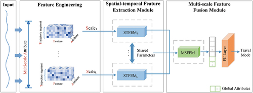
The proposed MSAF framework contains three principal components of feature engineering, a spatio-temporal feature extraction module (STFEM), and a multi-scale feature fusion module (MSFFM), as shown in Figure 3. 1) Feature engineering: This partially uses different time windows to dynamically segment the trajectory into multiple scales and extracts local features at each scale to reveal patterns and regularities in the trajectory data. 2) STFEM: This module extracts spatio-temporal features by fusing local and global attributes at multiple scales to capture motion state changes and spatio-temporal dependencies of trajectories at different scales. 3) MSFFM: This part uses an attribute attention model to adaptively learn the important weight of features at various scales to improve the accuracy of travel mode detection.

Figure 3. The network structure of MSAF.

4.2. Dynamic multi-scale local spatio-temporal feature extraction

This study employs a dynamic multiscale segmentation methodology to extract each GPS trajectory segment’s motion state and spatio-temporal characteristics. The feature engineering process shown in Figure 4 includes three steps: time window selection, multi-scale definition, and attribute computation. First, we analyzed the movement patterns associated with various travel modes to identify four time window scales that optimally accentuate the key features of trajectory segments. It is important to note that these time scales might differ across different trajectory datasets. By integrating these time windows with trajectory segments, a multi-scale structure was subsequently established to detect variations in the trajectory segments’ motion states across different temporal and spatial dimensions. This dynamic multi-scale segmentation approach involves dividing the trajectory into $2\mathit{k}+1$ segments by slicing $\mathit{k}$ pivotal trajectory segments using a sliding time window $\mathit{T}$. In the final step, comprehensive local and global multi-attribute analyses were performed for each trajectory segment.

Figure 4. The process of time window selection, multi-scale definition, and attribute calculation in feature engineering.

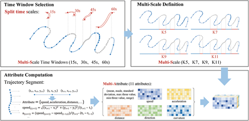
4.2.1. Time window definition

In this study, the time window $\mathit{T}$ denotes a fixed length of time ($\mathit{T}$=$\{\mathit{t}|\mathit{t}=15\mathrm{s},30\mathrm{s},45\mathrm{s},\mathit{\hspace{0.17em}}60\mathrm{s}\}$). Adjusting the time window allows the extraction of trajectory segments with minimal movement from the trajectory data, effectively dividing the entire trajectory into segments with identical motion states. Here, $\mathit{T}$ serves as a scale parameter that controls the granularity of trajectory segmentation. A short-time window is well suited for capturing brief changes in trajectory data and small-scale motion patterns, including momentary behaviors such as turning, acceleration, and deceleration. Shorter time windows allow the identification of short-term features, such as rapid changes in movement, traffic congestion, and frequent stopping points. Conversely, longer time intervals are often employed to capture prolonged patterns and large-scale movements in trajectory data. This approach aids in identifying the general features associated with various travel modes, such as commuting, long-distance driving, and subway travel.

4.2.2. Multi-scale definitions

This study defines multiscale by combining a trajectory segment $\mathit{K}$ value and a time window $\mathit{T}$ while applying a sliding time window to extract the most densely sampled segments from the trajectory data. Additionally, the trajectory $2\mathit{k}+1$ segments were divided to capture multi-scale motion characteristics while traveling. Features at different scales have distinct importance, and the critical feature scales are different for the various modes of travel. For instance, the trajectories of bus and subway trips usually have numerous lower-speed or stationary sections due to the stopping behavior at bus stops and subway stations. The low-speed segments can be effortlessly captured using various time windows and scales. As a result, the trajectory can be divided into segments with the same kinematic state. Therefore, by choosing a suitable time window, the changing characteristics of the motion states of different travel modes were accurately captured.

4.2.3. Attribute calculation

The segmented trajectory, $\mathit{T}$, can be denoted as $⟨s_1^{2k+1},s_2^{2k+1},\dots ,\mathit{\hspace{0.17em}}{s}_i^{2k+1},\dots ,s_{2k}^{2k+1},s_{2k+1}^{2k+1}⟩$, where each segment is represented by $s_i^{2k+1}$. For each segment, we then calculated five specific attributes: velocity, acceleration, distance, heading, and curvature. The corresponding statistical information was also obtained for each attribute. Velocity, for example, is comprised of 11 characteristics, including mean, median, standard deviation, maximum tristimulus, minimum tristimulus, and value range.

4.3. Multi-scale spatio-temporal attribute fusion network

4.3.1. Spatio-temporal feature extraction module

STFEM is designed to fuse local motion states with channel-level crosstalk and capture embedded spatio-temporal features from the input feature matrix at each spatial scale. It consists of the following components, as shown in Figure 5.

Figure 5. Spatio-temporal feature extraction module used in MSAF.

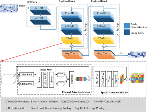
The 3D convolutional layer is where passages of trajectory segmentation are temporally ordered in time. This layer adds time dimension processing compared to the typical 2D convolution. Thus, 3D convolution may be executed concurrently in three dimensions (e.g. width, height, and time) to capture the characteristic representation of the input data in both space and time. In the spatial realm, 3D convolution can extract spatial structural information and capture the spatial correlation among pixels. In the temporal dimension, the 3D convolutional layer can learn about the dynamics of the input sequence of trajectory data.

Residual connectivity constitutes a crucial network structure in deep learning that aims to address the issues of gradient vanishing and explosion in deep networks while enhancing the network’s training effectiveness and generalization capability. By incorporating residual connections into each convolutional block, the network can seamlessly add the output values of a prior layer to those of a later layer, bypassing the need for convoluted nonlinear transformations. The benefit of this architecture lies in its ability to propagate the gradient to shallower layers via jump connections even as the number of network layer increases. This prevents the gradient from vanishing and subsequently enhances the model’s performance and training efficacy.

Since the travel modes assign distinct and varying importance to the features extracted from the convolutional layer, incorporating an attention mechanism in the travel mode recognition task empowers the model to assign higher attention weights to particular locations or channels, which elevates their importance. As shown in Figure 5, the Convolution Block Attention Module (CBAM) improves feature representation in convolutional neural networks by combining both channel and spatial attention functions. The channel attention is converted to a global feature vector for each channel’s feature map via a global average pooling operation. The vector then goes through two fully connected layers to ascertain the channel attention weights. These weights are later applied to the initial input feature map using channel-by-channel multiplication to obtain the calibrated feature map. The recalibrated feature maps undergo max-pooling and average-pooling operations along the channel dimensions to generate two spatial feature maps for the spatial attention mechanism. These two spatial feature maps experience a convolution operation with an activation function to obtain spatial attention weights, which are subsequently utilized to acquire the final feature map by applying them to the recalibrated feature map. Thus, the channel attention can be expressed as:

(7) $\mathit{Mc}\left(\mathit{F}\right)=\mathit{\sigma }\left(\mathit{MLP}\left(\mathit{AvgPool}\left(\mathit{F}\right)\right)+\mathit{MLP}\left(\mathit{MaxPool}\left(\mathit{F}\right)\right)\right)=\mathit{\sigma }\left(W_1\left(W_o\left(F_{avg}^C\right)\right)+\left(W_1\left(W_o\left(F_{max}^C\right)\right)\right)\right)$(7)

(8) $\mathit{Ms}\left(\mathit{F}\right)=\mathit{\sigma }\left(f^{7\ast 7}\left(\left[\mathit{AvgPool}\left(\mathit{F}\right)\right];\mathit{MaxPool}\left(\mathit{F}\right)]\right)\right)=\mathit{\sigma }(f^{7\ast 7}\left(\left[F_{avg}^s;F_{max}^s\right]\right)$(8)

where σ is the sigmoid operation, $f^{7\ast 7}$ denotes the size of the convolution kernel, and higher squared exponent values are better.

4.3.2. Multi-scale feature fusion module

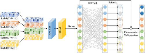
The substantial disparities in spatial characteristics and local motion states across distinct temporal and spatial scales cause them to make varied contributions to the ultimate identification. To address this issue, features for each object are integrated at all scales using the learned weights from a fusion module equipped with an attention mechanism.

The MSFFM operates as shown in Figure 6. First, the attribute attention model calculates the weights of the extracted features for each scale by implementing an attention mechanism, an attention network, or a probability distribution. The fusion of each scale feature is then achieved through the weighted multiplication of its corresponding weights. This method applies weighting to combine the contributions of various scale features, resulting in enhanced accuracy for recognizing different travel modes.

Figure 6. Multi-scale feature fusion module used in MSAF.

5. Results and discussion

5.1. Experimental dataset

This study validates the performance of the MSAF model using the GeoLife Trajectories dataset (Zheng et al. 2008, 2009; Zheng, Xie, and Ma 2010) and the SHL dataset. The GeoLife Trajectories dataset from Microsoft Research Asia, including the travel trajectories of 182 users over 5 years, features extensive volunteer participation and diverse transportation modes. To determine the modes of transportation, we selected five main categories based on the dataset author’s recommendations, which include walking, biking, bus, car, and subway. The sample sizes for each mode of travel are as follows: walking 2538 segments, biking 1143 segments, bus 1437 segments, subway 382 segments, and car 603 segments. The SHL dataset includes travel trajectories for two users over 3 days and one user over 75 days, characterized by extended periods of continuous data collection.

5.2. Experimental settings

5.2.1. Computing environment

All experiments in this paper were carried out on a workstation equipped with an Intel(R) Xeon(R) W-2225 CPU clocked at 4.10 GHz, 16 GB RAM, and an NVIDIA Quadro RTX 6000 graphics card. Deep learning models have been implemented utilizing the Python programming language and the open-source PyTorch framework (version 3.8.0) on the Windows 10 operating system.

5.2.2. Baseline methods

In this experiment, we selected six baseline methods for comparison, including (a) DT, (b) SVM, (c) XGBoost, (d) RF, (e) CNN, and (f) CNN-attention. Since DT, SVM, XGBoost, and RF cannot directly process the feature data, we compress the feature map into a one-dimensional input. To determine the ideal impulse parameters for the baseline models, we also employed a five-fold cross-validation and grid search approach.

5.2.3. Evaluation

To facilitate comparison of classification model performance, precision, recall, F-score, and confusion matrix are utilized as evaluation metrics.

5.2.4. Implementation details

We use PyTorch and Keras to construct the model. Table 2 shows the structure of the model. The dataset is divided into training, validation, and test sets in a 6:2:2 ratio, and we ensure that the ratio of each model is consistent with the entire GeoLife dataset. The optimization function is Adam, with a weight decay function w of 0.0001, the batch size is 2, the epoch is 100, and the learning rate is set to 0.001.

Table 2. Model structure.

Modules	Blocks	Layers
STFEM	3D Convolution Block	[3*3] conv3D
	Residual Block	[3*3] conv*2
		GlobalAvgPool + [1*1] Conv + ReLU + [1*1] Conv + Sigmoid
		[3*3] conv(Shortcut)
	Pool Block	[2*2] AvgPool2d
MSFFM	Fully connected block	Fully connected*2
	Scale attention block	Fully connected + Tanh + Softmax

5.3. Results

5.3.1. Overall performance

To evaluate the prediction accuracy of the proposed MSAF model compared to the classical baseline models, Table 3 lists the TMI accuracy of the overall model performance at different time intervals. Findings reveal that the MSAF model consistently outperforms all baseline models on trajectories that employ various t-segmentation time scales. Specifically, the MSAF model achieves the highest prediction accuracy of 95.16% on the GeoLife dataset and 91.70% on the SHL dataset, with an average accuracy improvement ranging from 2.50% to 7.95% and 0.80–6.62%, respectively. Although other models (e.g. CNN-attention) also perform well, the MSAF model consistently outperforms them in most configurations. While incorporating additional motion attributes into the baseline model can enhance prediction performance, the model’s input structure poses challenges to effectively extracting motion features. Consequently, capturing the underlying spatio-temporal characteristics of complex trajectory data becomes challenging. The baseline model’s shallow structure also limits its ability to represent and effectively learn nonlinear patterns, particularly when complex trajectory data contain rich nonlinear relationships. In contrast, the MSAF model’s ability to handle multiple spatio-temporal features at different scales and capture finer details and variations results in more precise predictions across different spatio-temporal scales.

Table 3. Comparison of TMI accuracy with classical model for different time intervals.

Model	GeoLife dataset(%)				SHL dataset(%)
	15s	30s	45s	60s	15s	30s	45s	60s
DT	85.11	85.37	86.69	86.44	74.01	75.76	76.25	73.02
SVM	74.92	75.39	77.43	77.07	68.79	70.28	73.26	71.43
XGBoost	85.83	86.66	86.84	86.71	77.79	79.53	82.52	80.79
RF	86.62	87.70	88.12	87.13	82.52	84.01	84.76	85.50
CNN	88.85	90.16	90.66	90.52	87.43	88.67	88.92	89.42
CNN-attention	89.84	90.90	92.79	91.89	89.07	90.21	90.45	90.32
MSAF	92.87	94.02	95.16	93.36	90.18	90.94	91.70	90.45

5.3.2. Effects of MSAF

Table 4 displays the confusion matrix for the MSAF and CNN-attention baseline model. Elements without parenthesis represent the results of the CNN-attention model, and those within the parenthesis belong to the MSAF model. Notably, the upper-diagonal values within the parentheses are significantly greater than those outside, indicating that the MSAF model correctly classified more samples than the CNN-attention model. By calculation, the average accuracy of MSAF is 95.16%, which exceeds the accuracy of the CNN-attention model at 92.79%.

Table 4. Confusion matrix for MSAF and baseline CNN-attention model.

CNN-attention (MSAF)		Predicted class
		Walk	Bike	Bus	Subway	Car
Actual class	Walk	486(499)	17(7)	5(1)	0(0)	0(0)
	Bike	6(4)	208(214)	15(10)	0(0)	0(1)
	Bus	2(1)	4(5)	264(269)	6(0)	11(12)
	Subway	0(0)	0(0)	1(2)	70(70)	5(4)
	Car	0(0)	0(0)	14(12)	2(0)	104(109)

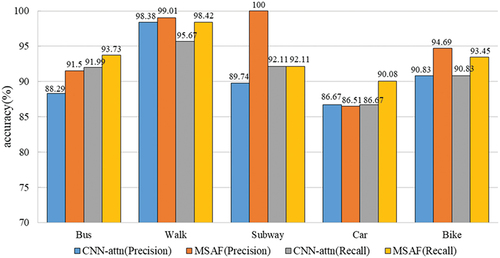
After comparing the confusion matrices of the MSAF and CNN-attention models, the recall and precision of these models are then illustrated. Figure 7 shows the distinctions in prediction accuracy and recall between the two models. Results indicate that MSAF has superior performance in detecting all modes of travel, especially walking, subway, and bus. The MSAF model significantly improved recall and precision, averaging 2.38% and 0.98%, respectively. Note that this dataset’s sample size for subway and car trips is smaller than that for the other three transportation methods. The MSAF model effectively addresses the issue of sample imbalance, resulting in an 8% and 8.59% increase in recognition accuracy and a 1.32% and 9.91% improvement in recall, respectively. This underscores its enhanced robustness.

Figure 7. Recall and precision of MSAF and baseline CNN-attention model.

The proposed model was then evaluated by comparing accuracy with related studies that utilized the GeoLife project dataset. In these studies, Endo et al. (2016) initially employed DNN, while (H. Wang et al. 2017) further integrated trajectory-level manual features with deep features. Subsequently, Dabiri and Heaslip (2018) introduced CNN and organized trajectory features into a multi-channel format. Following this, Jiang et al. (2020) utilized CNN to extract multi-scale local features. Li et al. (2020) balanced the dataset by generating adversarial networks. Li et al. (2021) combines GIS information. Kim, Kim, and Lee (2022) combined CNN and long short-term memory (LSTM) networks. Zeng et al. (2023) constructed trajectories into sequences and used the seq2seq model for classification. Ma et al. (2023) further utilized multi-attribute-multi-scale-multi-target image features. Table 5 shows that the proposed model achieves the best performance.

Table 5. Comparison of accuracy with related studies.

Model	Test accuracy(%)
(Endo et al. 2016)	67.9
(Wang et al. 2017)	74.1
(Dabiri and Heaslip 2018)	84.8
(Jiang et al. 2020)	83.9
(Li et al. 2020)	86.7
(Li et al. 2021)	91.1
(Kim, Kim, and Lee 2022)	92.1
(Zeng et al. 2023)	85.23
(Ma et al. 2023)	92.25
MSAF	95.16

5.3.3. Effect of multi-scale attributes

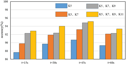
Figure 8 shows the performance comparison of different scale combinations, assessing how multi-scale feature combinations impact the MSAF model across various time windows. The detailed scheme settings are listed in Table 6. Different combinations of multiple segmentation scales are used under each time window $\mathit{t}$, respectively. The efficiency of multiscale feature fusion was determined by comparing the impact of various time windows and amalgamations of multiscale features. Findings reveal that the model’s accuracy scales up with increased time windows. However, the accuracy declines when the time window exceeds 60s, possibly because buses and subways usually halt for 45-60 s, which impacts accuracy. Shorter time windows can effectively capture these periodic stopping features, but longer time windows may encompass portions of the travel process that introduce noise and reduce the model’s identification accuracy. The model’s accuracy improved progressively as the combination of multi-scale features increased. This is because features from different scales can complement each other, thereby more comprehensively capturing the characteristics of travel modes and achieving optimal performance in travel mode recognition.

Table 6. The schematic setup for verifying the effectiveness of multi-scale feature combinations.

Case	T	Segmenting methods
Case 1	t=15s	K5_15
		K5_15, K7_15
		K5_15, K7_15, K9_15
		K5_15, K7_15, K9_15, K11_15
Case 2	t=30s	K5_30
		K5_30, K7_30
		K5_30, K7_30, K9_30
		K5_30, K7_30, K9_30, K11_30
Case 3	t=45s	K5_45
		K5_45, K7_45
		K5_45, K7_45, K9_45
		K5_45, K7_45, K9_45, K11_45
Case 4	t=60s	K5_60
		K5_60, K7_60
		K5_60, K7_60, K9_60
		K5_60, K7_60, K9_60, K11_60

Figure 8. Performance comparison of different scale combinations.

Note what happens if the trajectory with some sampling points and a short sampling time cannot be segmented into the desired segments by the time window $\mathit{t}$. For example, using the time window $\mathit{t}$ to extract $\mathit{k}$ trajectory segments, segmenting the trajectory into $2\mathit{k}+1$ segments requires a minimum trajectory segmentation into $2\mathit{k}+3$ segments. In this case, we progressively split the trajectory from the time window $\mathit{t}-1$ until the required number of subsections was achieved.

5.3.4. Ablation experiments

To thoroughly evaluate the contribution of each component within the MSAF model, including Residual Learning (RL) and CBAM applied in STFEM and Scale Attention (SA) used in MSFFM, we conducted a series of ablation experiments. As shown in Table 7, the experimental results indicate that these three components in the MSAF model effectively enhance the accuracy of travel mode identification.

Table 7. Ablation experiments with MSAF.

Module	Configure	Test accuracy(%)
STFEM	Without-RL	91.67
	Without-CBAM	92.46
MSFFM	Without-SA	93.03
	MSAF	95.16

6. Conclusion

Existing methods of TMI often rely on data resampling and integrating GIS information to improve accuracy, but this comes at the cost of losing original information and increasing experimental complexity. This study adopts a novel approach that uses raw GPS trajectories to recognize travel modes. The proposed method dynamically extracts multi-scale features from these trajectories, presenting a new deep-learning framework named MSAF. The method effectively captures multi-scale temporal and spatial features from travel trajectories while addressing challenges, such as sample imbalance and remaining highly adaptable without fixed requirements for trajectory length or sampling points.

Future work can be directed toward three main parts.

1. Fusing multi-source geographic information data: Explore effective methods for combining various types of geographic data, including rail routes, bus and metro stops, points of interest, land use, and transportation road networks. This fusion would involve developing more advanced data preprocessing and enhancement techniques to eliminate data redundancy and inconsistencies, thereby improving data quality. Such improvements will enable more accurate recognition of travel modes.

2. Physical model integration with deep learning: combining model-driven and data-driven approaches using perceptual-physical prior with deep learning. This involves using deep learning to learn features from large-scale trajectory data while incorporating physical constraints to enhance model interpretability, accuracy, and generalization ability.

3. Optimizing untagged data utilization: Untagged data, such as cell phone signaling data, contain significant information like the device’s location, speed, and spatial movement. Considering the scarcity of publicly accessible tagged GPS positioning datasets, techniques such as semi-supervised, self-supervised, and migratory learning can fully exploit the potential of unlabeled data.

Disclosure statement

No potential conflict of interest was reported by the author(s).

Data availability statement

The GeoLife dataset can be found at https://www.microsoft.com/en-us/research/publication/geolife-gps-trajectory-dataset-user-guide/. The Sussex-Huawei Locomotion dataset can be downloaded from http://www.shl-dataset.org/.

Additional information

Funding

This work is supported by the Strategic Priority Research Program of the National Natural Science Foundation of China [grant number 42301523].

Notes on contributors

Kunkun Fan

Kunkun Fan is a master’s student at the Academy of Digital China (Fujian), Fuzhou University. His primary research interests include web text mining and traffic trajectory data mining.

Daichao Li

Daichao Li received the PhD degree from Institute of Geographic Sciences and Natural Resources Research, CAS. Her main research interests include spatiotemporal data mining, spatiotemporal knowledge graphs, and spatiotemporal data visualization and visual analysis.

Xinlei Jin

Xinlei Jin is a master’s student at the Academy of Digital China (Fujian), Fuzhou University. Her research interests include data management and Internet economy and big data analysis.

Sheng Wu

Sheng Wu received the PhD degree from Information Engineering University. He is currently a full professor in the Key Laboratory of Spatial Data Mining & Information Sharing of Ministry of Education, Fuzhou University. His research interests include big data analysis and visualization, big data mining, and web spatial behavior analysis.

References

- Dabiri, S., and K. Heaslip. 2018. “Inferring Transportation Modes from GPS Trajectories Using a Convolutional Neural Network.” Transportation Research Part C: Emerging Technologies 86:360–371. https://doi.org/10.1016/j.trc.2017.11.021.
- Dabiri, S., C. Lu, K. Heaslip, and C. K. Reddy. 2019. “Semi-Supervised Deep Learning Approach for Transportation Mode Identification Using GPS Trajectory Data.” IEEE Transactions on Knowledge and Data Engineering 32 (5): 1010–1023. https://doi.org/10.1109/TKDE.2019.2896985.
- Dabiri, S., N. Marković, K. Heaslip, and C. K. Reddy. 2020. “A Deep Convolutional Neural Network Based Approach for Vehicle Classification Using Large-Scale GPS Trajectory Data.” Transportation Research Part C: Emerging Technologies 116:102644. https://doi.org/10.1016/j.trc.2020.102644.
- Endo, Y., H. Toda, K. Nishida, and J. Ikedo. 2016. “Classifying Spatial Trajectories Using Representation Learning.” International Journal of Data Science and Analytics 2 (3): 107–117. https://doi.org/10.1007/s41060-016-0014-1.
- Gjoreski, H., M. Ciliberto, L. Wang, F. J. O. Morales, S. Mekki, S. Valentin, and D. Roggen. 2018. “The University of Sussex-Huawei Locomotion and Transportation Dataset for Multimodal Analytics with Mobile Devices.” Institute of Electrical and Electronics Engineers Access 6:42592–42604. https://doi.org/10.1109/ACCESS.2018.2858933.
- Gong, L., T. Morikawa, T. Yamamoto, and H. Sato. 2014. “Deriving Personal Trip Data from GPS Data: A Literature Review on the Existing Methodologies.” Procedia-Social and Behavioral Sciences 138:557–565. https://doi.org/10.1016/j.sbspro.2014.07.239.
- Guo, M., S. Liang, L. Zhao, and P. Wang. 2020. “Transportation Mode Recognition with Deep Forest Based on GPS Data.” Institute of Electrical and Electronics Engineers Access 8:150891–150901. https://doi.org/10.1109/ACCESS.2020.3015242.
- Hui, K. T. Y., C. Wang, A. Kim, and T. Z. Qiu. 2017. “Investigating the Use of Anonymous Cellular Phone Data to Determine Intercity Travel Volumes and Modes.” https://trid.trb.org/View/1438460.
- Jahangiri, A., and H. A. Rakha. 2015. “Applying Machine Learning Techniques to Transportation Mode Recognition Using Mobile Phone Sensor Data.” IEEE Transactions on Intelligent Transportation Systems 16 (5): 2406–2417. https://doi.org/10.1109/TITS.2015.2405759.
- James, J. Q. 2020. “Travel Mode Identification with GPS Trajectories Using Wavelet Transform and Deep Learning.” IEEE Transactions on Intelligent Transportation Systems 22 (2): 1093–1103. https://doi.org/10.1109/TITS.2019.2962741.
- Jiang, G., S. Lam, P. He, C. Ou, and D. Ai. 2020. “A Multi-Scale Attributes Attention Model for Transport Mode Identification.” IEEE Transactions on Intelligent Transportation Systems 23 (1): 152–164. https://doi.org/10.1109/TITS.2020.3008469.
- Jiang, Z., A. Huang, G. Qi, and W. Guan. 2023. “A Framework of Travel Mode Identification Fusing Deep Learning and Map-Matching Algorithm.” IEEE Transactions on Intelligent Transportation Systems. https://doi.org/10.1109/TITS.2023.3250660.
- Ju, H., G. Zeng, and S. Zhang. 2024. “Inter-Provincial Flow and Influencing Factors of Agricultural Carbon Footprint in China and Its Policy Implication.” Environmental Impact Assessment Review 105:107419. https://doi.org/10.1016/j.eiar.2024.107419.
- Kim, J., J. H. Kim, and G. Lee. 2022. “GPS Data-Based Mobility Mode Inference Model Using Long-Term Recurrent Convolutional Networks.” Transportation Research Part C: Emerging Technologies 135:103523. https://doi.org/10.1016/j.trc.2021.103523.
- Li, J., X. Pei, X. Wang, D. Yao, Y. Zhang, and Y. Yue. 2021. “Transportation Mode Identification with GPS Trajectory Data and GIS Information.” Tsinghua Science and Technology 26 (4): 403–416. https://doi.org/10.26599/TST.2020.9010014.
- Li, L., J. Zhu, H. Zhang, H. Tan, B. Du, and B. Ran. 2020. “Coupled Application of Generative Adversarial Networks and Conventional Neural Networks for Travel Mode Detection Using GPS Data.” Transportation Research Part A: Policy and Practice 136:282–292. https://doi.org/10.1016/j.tra.2020.04.005.
- Ma, Y., X. Guan, J. Cao, and H. Wu. 2023. “A Multi-Stage Fusion Network for Transportation Mode Identification with Varied Scale Representation of GPS Trajectories.” Transportation Research Part C: Emerging Technologies 150:104088. https://doi.org/10.1016/j.trc.2023.104088.
- Nawaz, A., H. Zhiqiu, W. Senzhang, Y. Hussain, I. Khan, and Z. Khan. 2020. “Convolutional LSTM Based Transportation Mode Learning from Raw GPS Trajectories.” IET Intelligent Transport Systems 14 (6): 570–577. https://doi.org/10.1049/iet-its.2019.0017.
- Patterson, D. J., L. Liao, D. Fox, and H. Kautz. 2003. “Inferring High-Level Behavior from Low-Level Sensors.” Ubiquitous Computing: 5th International Conference, 73–89. Seattle, WA, USA. October 12–15, Proceedings 5. Springer Berlin Heidelberg, 2003: https://doi.org/10.1007/978-3-540-39653-6_6.
- Sadeghian, P., J. Håkansson, and X. Zhao. 2021. “Review and Evaluation of Methods in Transport Mode Detection Based on GPS Tracking Data.” Journal of Traffic & Transportation Engineering( English Edition)8 (4): 467–482. https://doi.org/10.1016/j.jtte.2021.04.004.
- Shen, L., and P. R. Stopher. 2014. “Review of GPS Travel Survey and GPS Data-Processing Methods.” Transport Reviews 34 (3): 316–334. https://doi.org/10.1080/01441647.2014.903530.
- Stopher, P., E. Clifford, J. Zhang, and C. FitzGerald. 2008. “Deducing Mode and Purpose from GPS Data.” https://ses.library.usyd.edu.au/handle/2123/19552.
- Stopher, P. R., Q. Jiang, and C. FitzGerald. 2005. “Processing GPS Data from Travel Surveys.” In 28th Australasian Transport Research Forum, ATRF 05, Sydney, NSW, Australia.
- Tsui, S. Y. A., and A. S. Shalaby. 2006. “Enhanced System for Link and Mode Identification for Personal Travel Surveys Based on Global Positioning Systems.” Transportation Research Record 1972 (1): 38–45. https://doi.org/10.1177/0361198106197200105.
- Vincent, P., H. Larochelle, I. Lajoie, Y. Bengio, P. Manzagol, and L. Bottou. 2010. “Stacked Denoising Autoencoders: Learning Useful Representations in a Deep Network with a Local Denoising Criterion.” Journal of Machine Learning Research 11 (12): 3371–3408.
- Wang, C., H. Luo, F. Zhao, and Y. Qin. 2020. “Combining Residual and LSTM Recurrent Networks for Transportation Mode Detection Using Multimodal Sensors Integrated in Smartphones.” IEEE Transactions on Intelligent Transportation Systems 22 (9): 5473–5485. https://doi.org/10.1109/TITS.2020.2987598.
- Wang, H., G. Liu, J. Duan, and L. Zhang. 2017. “Detecting Transportation Modes Using Deep Neural Network.” IEICE Transactions on Information and Systems 100 (5): 1132–1135. https://doi.org/10.1587/transinf.2016EDL8252.
- Wang, L., H. Gjoreski, M. Ciliberto, S. Mekki, S. Valentin, and D. Roggen. 2019. “Enabling Reproducible Research in Sensor-Based Transportation Mode Recognition with the Sussex-Huawei Dataset.” Institute of Electrical and Electronics Engineers Access 7:10870–10891. https://doi.org/10.1109/ACCESS.2019.2890793.
- Xiao, G., Q. Cheng, and C. Zhang. 2019. “Detecting Travel Modes from Smartphone-Based Travel Surveys with Continuous Hidden Markov Models.” International Journal of Distributed Sensor Networks 15 (4): 1550147719844156. https://doi.org/10.1177/1550147719844156.
- Xiao, Z., Y. Wang, K. Fu, and F. Wu. 2017. “Identifying Different Transportation Modes from Trajectory Data Using Tree-Based Ensemble Classifiers.” ISPRS International Journal of Geo-Information 6 (2): 57. https://doi.org/10.3390/ijgi6020057.
- Yamada, Y., A. Uchiyama, A. Hiromori, H. Yamaguchi, and T. Higashino. 2016. “Travel Estimation Using Control Signal Records in Cellular Networks and Geographical Information.” 2016 9th IFIP Wireless and Mobile Networking Conference (WMNC), IEEE, 138–144. https://ieeexplore.ieee.org/abstract/document/7543981.
- Yang, X., K. Stewart, L. Tang, Z. Xie, and Q. Li. 2018. “A Review of GPS Trajectories Classification Based on Transportation Mode.” Sensors (Basel) 18 (11): 3741. https://doi.org/10.3390/s18113741.
- Zan, D., B. Chen, F. Zhang, D. Lu, B. Wu, B. Guan, W. Yongji, and J. Lou. 2023. “Large Language Models Meet NL2Code: A Survey.” arXiv Preprint arXiv: 7443–7464. https://doi.org/10.48550/arXiv.2212.09420.
- Zeng, J., Y. Yu, Y. Chen, D. Yang, L. Zhang, and D. Wang. 2023. “Trajectory-As-A-Sequence: A Novel Travel Mode Identification Framework.” Transportation Research Part C: Emerging Technologies 146:103957. https://doi.org/10.1016/j.trc.2022.103957.
- Zhang, C., Y. Zhu, C. Markos, S. Yu, and J. Q. James. 2021. “Toward Crowdsourced Transportation Mode Identification: A Semisupervised Federated Learning Approach.” IEEE Internet of Things Journal 9 (14): 11868–11882. https://doi.org/10.1109/JIOT.2021.3132056.
- Zhang, L., T. Cheng, T. Yue, S. Li, and J. P. Wilson. 2024. “Quantitative Analysis of Spatiotemporal Coverage and Uncertainty Decomposition in OCO-2/3 XCO2 Across China.” Atmospheric Environment: 120636. https://doi.org/10.1016/j.atmosenv.2024.120636.
- Zhang, R., P. Xie, C. Wang, G. Liu, and S. Wan. 2019a. “Classifying Transportation Mode and Speed from Trajectory Data via Deep Multi-Scale Learning.” Computer Networks 162:106861. https://doi.org/10.1016/j.comnet.2019.106861.
- Zhang, R., P. Xie, C. Wang, G. Liu, and S. Wan. 2019b. “Understanding Mobility via Deep Multi-Scale Learning.” Procedia Computer Science 147:487–494. https://doi.org/10.1016/j.procs.2019.01.251.
- Zheng, Y., Q. Li, Y. Chen, X. Xie, and W. Ma. 2008. “Understanding Mobility Based on GPS Data.” Proceedings of the 10th international conference on Ubiquitous computing, 312–321. https://doi.org/10.1145/1409635.1409677.
- Zheng, Y., X. Xie, and W. Ma. 2010. “GeoLife: A Collaborative Social Networking Service Among User, Location and Trajectory.” IEEE Data Eng Bull 33 (2): 32–39. https://citeseerx.ist.psu.edu/document?repid=rep1&type=pdf&doi=24ccdcba118ff9a72de4840efb848c7c852ef247 .
- Zheng, Y., L. Zhang, X. Xie, and W. Ma. 2009. ““Mining Interesting Locations and Travel Sequences from GPS Trajectories.” Proceedings of the 18th international conference on World wide web, 791–800. https://doi.org/10.1145/1526709.1526816.
- Zhu, Y., Y. Liu, J. Q. James, and X. Yuan. 2021. “Semi-Supervised Federated Learning for Travel Mode Identification from GPS Trajectories.” IEEE Transactions on Intelligent Transportation Systems 23 (3): 2380–2391. https://doi.org/10.1109/TITS.2021.3092015.