Classification of boreal macrotidal littoral zone habitats in the Gulf of Maine: comparison of IKONOS and CASI multispectral imagery

Abstract

Increasingly, remote sensing has become a useful tool for mapping and measuring terrestrial and aquatic environments. Advances in the spatial and spectral resolution of satellite-borne sensors have allowed affordable investigations of littoral macrotidal coastal systems that previously required more costly aircraft-based imagery. In this communication, we compare the results from analysis of a 4 m spatial resolution, multispectral IKONOS satellite image of the intertidal habitats of Islesboro, Maine, USA with that of an aerial compact airborne spectral imager survey of the same regions captured 4 years earlier. There was 72% agreement between the surveys in spite of the temporal gaps between the images. Accuracy varied by habitat class and the perceived error can be assigned to temporal and definitional issues rather than basic acquisition and analytic protocols. Most of the error can be explained by: (1) inadequacy of training sites, (2) temporal variations and (3) class definitions. We conclude that IKONOS imagery provides sufficient spatial and spectral resolution to map and monitor diverse intertidal habitats as found in the macrotidal Gulf of Maine.

Keywords:

• intertidal
• IKONOS
• CASI
• comparisons
• habitats

1. Introduction

Remote sensing has become a widely used tool in environmental research with application in most facets of oceanographic research. Moderate-resolution sensors such as Landsat TM, MSS and ETM+ have been applied successfully to broad habitats such as coral reef systems, salt marshes and sea grasses (Ackleson and Klemas 1987, Ferguson and Korfmacher 1997, Mumby et al. 2004). The littoral zone of the macrotidal Gulf of Maine is particularly well suited to the application of remote sensing techniques as the habitats can be imaged without a confounding water column. We have used remote sensing at several spatial scales to address ecological questions in this region, including AVHRR (1 km thermal resolution), Landsat TM (30 m multispectral) and compact airborne spectral imager (CASI) (4 m multispectral) (Larsen 1985, Larsen and Erickson 1998, Larsen et al. 2004). The utility of remote sensing in nearshore and, especially, intertidal regions, however, has been somewhat restricted for several reasons, including the often narrow and spatially limited nature of the environment.

Advanced satellite-based imaging systems with increasing spatial and spectral resolutions are now available for application to remote sensing of terrestrial and aquatic environments. Space-based products can be obtained with spatial resolution on the order of metres to support studies in heterogeneous environments (Mumby and Edwards 2002, Andrefouet et al. 2002, Malthus and Mumby 2003). Despite these advances, problems still facing coastal researchers in the application of satellite products with repeat coverage cycles of 9–14 days include: (1) optimization of sensor signal to noise ratio for imaging aquatic versus terrestrial regions; (2) limited availability of spectrally relevant bands; and (3) failure of ascent/descent timing of polar orbiting satellites to match the occurrence of the lowest tides in many regions.

Our first major effort to map and classify the highly diverse and ecologically rich intertidal habitats of the Gulf of Maine utilized CASI, flown in August 1997 at low altitude on a small aircraft to image regions of the intertidal zone around Islesboro, Maine, in Penobscot Bay (Larsen and Erickson 1998). CASI has been used extensively to study sea grasses (Mumby et al. 1997), coral reefs (Mumby et al. 1998), mangroves (Green et al. 1998) and coarse intertidal habitat classes (Thomson et al. 1998a,b). A 4 m resolution mosaic of Islesboro Island, Maine (Figure 1) was produced using 10 spectral bands (Figure 2). A supervised classification of intertidal pixels was completed using 18 ecologically defined non-water classes ranging from sediment to macroalgae and marsh to upland. Overall accuracy was determined to be 81%. Although the quality of the results of this study was excellent, the cost for a single survey was prohibitive in terms of using CASI products for change analysis or as a monitoring tool. Subsequently, we employed low cost, synoptic Landsat TM imagery to input the area of primary producer groups into an energy-based ecological model developed for Cobscook Bay, another macrotidal estuary in the Gulf of Maine (Campbell 2004, Larsen et al. 2004). This too proved successful on the spatial scale at which we were working. The 30 m pixel size of Landsat, however, was not suitable to measure the finer scale heterogeneity characteristic of these littoral environments. We continued to look for image products that might combine the cost effectiveness of Landsat with the high spatial resolution of CASI.

Figure 1. The Islesboro study area on the central Maine coast, USA.

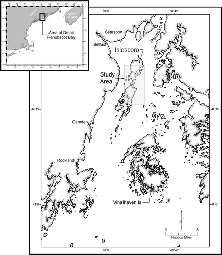
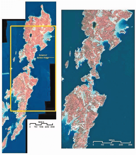
Figure 2. CASI (left) and IKONOS (right) images of Islesboro, Maine; yellow box indicates extent of IKONOS image.

This article presents the results of an intertidal zone classification produced using an IKONOS Geo image of Islesboro, Maine (Figure 1), and compares the results with those from the CASI study that occurred 4 years earlier. The purpose of this work is to demonstrate the utility of affordably-priced, high-resolution satellite imagery for monitoring large-scale, heterogeneous, intertidal marine habitats without the loss of classification accuracy. It is recognized that although these products offer substantial cost savings for the base imagery, the extensive nature of the image processing required to produce the classification and the cost of associated software may still be prohibitive for many potential end users.

2 Methods

2.1 Habitat classification scheme

The intertidal habitat classification scheme developed by Larsen and Erickson (1998) in support of their CASI survey of Penobscot Bay was utilized. This scheme was derived from general and Gulf of Maine specific classification protocols developed for a number of purposes (Cowardin et al. 1979, Maine State Planning Office 1983, Larsen and Doggett 1985, Dethier 1990, Brown 1993, Bailey et al. 1993). In brief, eight vegetative and 10 geological classes were defined (Table 1). Vegetative classes required at least 25% coverage; otherwise the site was characterized by the underlying substrate.

Table 1. Basic ecological definitions of eight intertidal vegetation classes and 10 substrate classes.

Intertidal vegetation classes	An area is assigned to be a vegetation class if 25% or more of the surface is covered by vegetation. When the dominant plant type exceeds 75% of the cover surface, the site is assigned to one of the ‘pure’ vegetation classes described below; otherwise it is assigned to mixed algae.
Brown algae	Algae belonging to the Division Phaeophyta except the kelps (see below). The principal members of this class are the rockweeds Ascophyllum and Fucus.
Green algae	Algae belonging to the Division Chlorophyta. Enteromorpha and Ulva are the most common genera.
Red algae	Algae belonging to the Division Rhodophyta. Red algae occur most abundantly in a band along the sublittoral fringe.
Kelp	Algae belonging to the Division Phaeophyta, Order Laminariales, i.e. a brown algal group. They are separated from the rockweeds because they occur in a different ecological context, the sublittoral fringe, and have distinct management considerations.
Mixed algae	Areas where several plant groups co-exist, but no one type contributes more than 75% surface cover.
Submerged aquatic vegetation (SAV)	Operationally, SAV beds consist of the rooted, vascular plants Zostera marina, commonly called eelgrass, and Ruppia maritima, known as widgeon grass.
Salt marsh	Salt-tolerant, emergent wetland plants; principally Spartina alterniflora and Spartina patens. Several subdominant species occur especially at higher marsh levels. Freshwater marshes are excluded from this study.
Spits and berms	Elongate, geological features of coarse sediment capped by supratidal plant communities influenced by salt spray.
Substrate classes	Substrate classes describe the non-living substrata of the environments surveyed.
Bedrock	Bedrock > 3 m diameter, can be various types of consolidated rock. Rock often has other materials overlying it or is found in conjunction with other types of substrata, and therefore, one can classify an area as rock if it has at least 50% cover of bedrock.
Boulder	Rocks > 256 mm but ≤ 3 m in diameter, i.e. those large enough not to be rolled by moderate wave action. Boulders are also associated with a variety of types of substrata from bedrock to mud. Any site with at least 75% boulders can be classified as boulder.
Cobble	Rocks > 64 mm but ≤ 256 mm; unstable. Cobble beaches are > 75% particles of this size.
Mixed coarse	Rock, boulders, cobbles, gravel, shell and/or sand. No one substratum type exceeds 75% surface cover; less than 50% cover by rock and boulders.
Gravel	Small rocks or pebbles > 2 but ≤ 64 mm in diameter. Habitats are deemed to have gravel substratum if 75% or more of the surface is gravel.
Mixed coarse and fines	Rocks, boulders and coarse and fine particles. No one substratum type exceeding 75% surface cover and less than 50% cover by rock and boulders.
Sand	Sediment particles ranging between 0.0625 and 2 mm in diameter. A habitat is defined as sand if 75% or more of the surface cover is sand.
Mixed fines	Mixture of sand and mud, with little gravel; likely to change seasonally.
Mud	Fine substrata < 0.0625 mm, usually mixed with organic matter. If a site has at least 75% surface cover of mud, it is classified as mud. Mud includes both silt and clay.
Artificial	Concrete blocks, tires, riprap, log booms, pilings, oyster culture, quarry tailings, roadways and others. This class accounts for a very small, but noticeable, percentage of Maine's intertidal habitat area.

2.2 Imagery

An IKONOS multispectral image, 4 m resolution, covering an area of approximately 66 km² on the island of Islesboro in Penobscot Bay, Maine (Figure 2) was acquired at 15:44 GMT on 12 September 2001. The image was processed to the standard geometrically corrected level, UTM coordinates, zone 19 and analysed to map and classify intertidal habitats (Table 2).

Table 2. Habitat class, classification code and signature distribution.

Habitat class	Code	Number of signatures
Brown algae	1	32
Mixed algae	2	4
Submerged aquatic vegetation	3	6
Spit/berm	4	3
Salt marsh	5	11
Cobble	6	2
Gravel	7	1
Mixed coarse/fine	8	13
Sand	9	3
Mud	10	3
Artificial	11	4
Water	12	22
Upland	13	0
Shadow	14	0
Total		104

The mosaicked CASI image (Figure 2) used for previous classification efforts provided an additional reference data source. The swath data used to create this image were acquired on 24–26 August 1997. Four metre pixels of 16-bit data using an 11-channel bandset between 470 and 875 nm resulted (Borstad Associates 1998).

Eleven of the defined habitat classes were found in the study area with sufficient regularity to be used as training sites. These classes were brown algae, mixed algae, submerged aquatic vegetation (SAV), spit/berm, salt marsh, cobble, gravel, mixed coarse and fine, sand, mud and artificial. Water, also a class in the CASI study, and Upland habitat training sites were added to the above classes. Because parts of the image were obscured, Shadow was added as a 14th class. Hence, the Islesboro IKONOS image was processed using 14 classes, 12 of which were pre-existing definitions of the 1997 CASI survey.

The image processing tasks were completed using the ERDAS Imagine image processing software package, version 8.6. Related GIS tasks utilized a suite of ESRI products, including workstation Arc/Info and ArcGIS products, versions 8.3.

To more easily compare the CASI-derived classifications and input data, the original IKONOS image was projected from UTM, WGS84 to UTM, NAD27, each having map units of metres. The projection was accomplished using the rigorous transformation option of the Imagine re-project routine.

We initially planned to use the land mask area of interest (AOI) created for the CASI work in the IKONOS image processing. However, spatial discrepancies remained following the datum transformation, thereby requiring that a new land mask AOI be generated based on the projected image. The new land mask was automated using the IKONOS image as a backdrop in one viewer whereas ‘linking’ the CASI image and its associated land mask AOI in a second viewer to help guide the on-screen delineation process.

The new land mask was used to subset the IKONOS image, retaining only those areas comprizing the intertidal zone and the subtidal region. Along most of the shoreline, a narrow strip of upland was also captured, to ensure that the entire intertidal zone was included in the processing. As with the CASI study, the subsetting was done to focus the processing on the nearshore areas of the imagery.

Image processing proceeded in an iterative manner. Classifications were produced and evaluated, keeping the satisfactory classes for inclusion in the final product, whereas using the poor classes and unclassified data to mask and reprocess the remaining problematic areas. Upon completion of a classification, each signature/class was individually highlighted and examined against the raw IKONOS image to determine its validity, then annotated as to whether or not it was acceptable.

We began the IKONOS classification using a supervised maximum likelihood approach (Leica Geosystems 2002), which required the acquisition of training sites and the development of class signatures. Signature development was initiated based on 45 training sites from the CASI study. The UTM coordinates for each of the sites were determined and used to generate a GIS point coverage. These points were then overlaid on the IKONOS image and signatures were generated using a seed pixel to grow spectrally similar regions. We required that each signature group contain at least 15 pixels and have a maximum standard deviation per band of five, presented as digital numbers in the Imagine signature statistics report. However, in habitat classes where the number of training sites was few (such as artificial), we were forced to relax these requirements.

The first classification was then generated using the initial signature set, with the process forcing assignment of each pixel into a specific class. The results revealed a lack of training sites in several categories, most notably the water and marsh classes. Numerous signatures were then added to the original training data to correct these deficiencies. Additional training sites were selected based on obvious spectral characteristics, image familiarity and other ancillary data sources such as Digital Orthophoto Quarterquads, 1 m resolution, obtained from the Maine Office of GIS web site at apollo.ogis.state.me.us.

A second classification was then performed utilizing the expanded set of training sites. However, in this iteration, not all pixels were forced into a particular class. A parallelepiped decision rule was used to restrict the classified pixels. Pixels whose data values extended beyond the parallelepiped limits were left unclassified, whereas pixels in overlap regions of the parallelepipeds were assigned using the parametric, maximum likelihood decision rule. This approach was used to classify only those pixels that were most likely represented by the existing signatures.

The unclassified pixels from the second classification were used to mask the image, producing a markedly speckled data set. This masked image was then used as the input for an unsupervised classification using the Imagine isodata routine, yielding 30 clusters along with corresponding signatures. The classification was evaluated, labelled (i.e. each pixel cluster coded) and the signatures added to the overall signature data set used in previous, supervised classifications. The final signature set (Table 2) contained 104 signatures available for a more comprehensive classification.

The original land masked IKONOS image was then classified, using the maximum likelihood algorithm with the 104 signatures described above. In this iteration, each pixel was assigned to a signature/class. The resulting classification was evaluated, whereby each signature/class was highlighted, individually inspected, and then coded to reflect its suitability in the final data set. Those pixels deemed suitable were retained, whereas the unacceptable signature/classes were identified and used to mask the image for further processing. These problematic signatures typically produced classes that included the target feature as well as other materials that did not belong. For example, many of the marsh signatures included non-marsh areas, thus requiring additional processing to separate the co-mingled features. In cases where the feature separation was obvious and consistent (such as between brown algae and upland habitats), a simple recode using AOI's was adequate to address the problem. In areas where conditions were less straightforward, we attempted to separate the classes using the spectral approaches described below.

Following the evaluation and editing of the supervised classification, we masked the image, retaining those pixels deemed unsuitably classified by the previous iteration. Because of the speckling produced with such a masking process (i.e. the pixels are not necessarily contiguous, making it more difficult to group a training site into a signature), an unsupervised classification was utilized. Again, the Imagine isodata routine was run on the masked image to produce a data set with 20 clusters. Each cluster was then individually evaluated and coded as to its proper category. As with the previous classification, there was some mixing of classes. One notable problem was the assignment of upland shadows to the water class. These areas were edited using the on screen AOI technique previously mentioned. The results of the supervised and unsupervised classifications were then merged to create the final classification containing the 11 classes of intertidal habitats, water, upland and shadow.

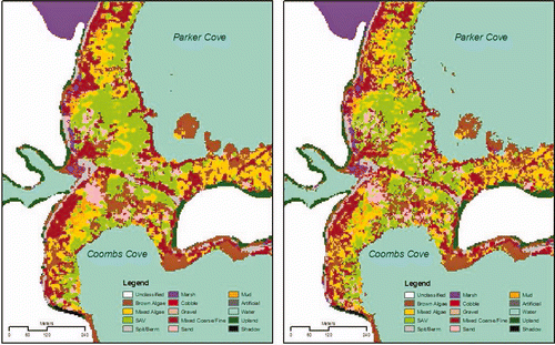
The final classification exhibited numerous single pixels scattered throughout the image. Because little confidence is typically associated with these individual pixels, filtering algorithms are often used to remove them or blend them into the surrounding classes. We tried two different approaches to smooth the final classification. The first was a simple 3 × 3 majority filter available through the Imagine interface. This filter produced a visually pleasing appearance; however, it had a marked effect on narrow, linear features such as the spit/berm class. We therefore used a combination of filters available in the Arc/Info GRID environment-grouping pixels into regions by way of orthogonal connections and then filtering only those single or double pixels not attached to a larger region. This technique preserved linear features while eliminating scattered, single pixels. Figure 3 compares the two filtering methods in areas around Coombs and Parker Coves. The differences in the two filtering approaches are most notable in the cobble class, where the 3 × 3 filtering method all but eliminated the cobble pixels while the region-group approach maintained some of the linear shapes in that class.

Figure 3. Classified data set filtered using the 3 × 3 majority filter (left) and the ESRI Arc/Info GRID region-group and majority filter (right).

One hundred and eighty-three assessment sites were randomly selected to evaluate the efficacy of the image processing. Examination of the images provided unambiguous positive results for all of the water sites, most of the upland sites and many of the brown algae sites. All of the remaining sites were visited and evaluated by project staff in September, November and December 2003, i.e. two-plus years after the satellite image was captured. Each site was placed into the most appropriate of 20 classes, i.e. the 18 classes of Larsen and Erickson (1998) plus water and upland, based on the field evaluation.

3 Results

The results of a deterministic accuracy assessment are presented in Table 3. The deterministic error matrix was constructed by plotting the IKONOS classifications against the results of field evaluations made 24–27 months after the image was captured. The table is asymmetric because the field evaluation encountered four ecological classes for which there had been insufficient training sites. Overall deterministic accuracy was then estimated by dividing the sum of the site counts on the main axis, i.e. where the remote sensing and field results were in absolute agreement, and dividing by the total number of accuracy assessment sites. In this case, there was a 72% agreement between the data sets. One hundred thirty-one sites were correctly assigned to the proper class by the remote sensing procedure and 52 sites were assigned to incorrect classes.

Table 3. Deterministic accuracy assessment of Islesboro, Maine sites.

	Ground reference
	Brown	Mixed algae	SAV	Spit/berm	Salt marsh	Cobble	Gravel	Mixed C/F	Sand	Mud	Artificial	Water	Upland	Ledge	Mixed coarse	Shells	Other	Row total
Traditional
Brown	15 (88%/100%)																	15
Mixed algae	1	8 (89%/53%)		1					3	1							1	15
SAV			7 (100%/58%)						4	1								12
Spit/berm		1		1 (25%/7%)			5				2			3	3			15
IKONOS
Salt marsh					11 (100%/100%)													11
Cobble						12 (100%/80%)		2	1									15
Gravel				1			6 (50%/40%)	2	1		3				1	1		15
Mixed C/F								9 (69%/90%)								1		10
Sand									15 (52%/100%)									15
Mud	1						1		4	7 (78%/47%)	1						1	15
Artificial				1					1		10 (62%/67%)			3				15
Water												13 (100%/100%)						13
Upland													17 (100%/100%)					17
Column total	17	9	7	4	11	12	12	13	29	9	16	13	17	6	4	2	2
Values within parenthesis represent producer's and user's accuracies for principal habitat classes.
Four classes representing 14 AA sites had no training sites. They explain 27% of observed error.

The adequacy of the classification process for individual classes may be evaluated by computing two other accuracy measures, the producer's accuracy and the user's accuracy (Congalton 1991). Error matrices for each of these are presented in Table 3. The classes of brown algae, salt marsh, cobble, water and upland exhibited high producer's and user's accuracy indicating that the procedures accurately and reliably interpreted the radiological signals received by the IKONOS satellite. Eight other classes, however, were problematic in terms of producer's or user's accuracy or both. Full evaluation of these errors of commission and omission are needed to understand the strengths and weaknesses of the IKONOS intertidal survey (Congalton and Green 1999).

4 Discussion

Examination of the producer's and user's accuracy matrices identifies five habitats that appear to be handled particularly well by the data acquisition and analysis protocols employed (Table 3). Examination of these values against the background of our field knowledge convinces us that the majority of the perceived error can be assigned to one of the three areas peculiar to temporal and definitional issues rather than to the basic data acquisition and analysis protocols. These areas are: (1) inadequacy of training sites, (2) temporal variations and (3) class definitions. Each type of error will be discussed below.

1. Inadequacy of training sites – The northern Islesboro subregion of the CASI survey was chosen for IKONOS evaluation because of the existence of a diversity of densely packed, accessible habitat types. All habitats, however, were not common enough to have sufficient training sites. Examination of the total error matrix indicates that there were 14 randomly chosen accuracy assessment sites that the field evaluators believed should be placed in one of the four classes that were not included in the training procedure, hence, the asymmetrical matrix (Table 3). These classes were bedrock, mixed coarse, shells and other. We have considered these determinations, which constitute 27% of the total error, to be incorrect in the overall accuracy assessment of 72%. It could be argued, however, that because these classes were not represented in the training sites, the computer processing correctly placed them into the available classes with the most similar spectral signals. Considering these sites to be correctly classified raises the overall accuracy assessment to a respectable 79%. Deleting them from the analysis altogether produces an accuracy assessment of 78%.

2. Temporal variations – Seasonal variations are pronounced in the Gulf of Maine and two of the classes with low producer's or user's accuracies, mixed algae and SAV, have strong seasonal components. Each is characterized, at least in part, by the presence of plant species with seasonal manifestations. The mixed algae class, by definition, contains a mix of species including the annual and ephemeral green algae Ulva and Enteromorpha. During the November and December field work, these species would not be present and the sites without co-occurring perennial species would be characterized by the underlying sediments, either sand or mud. Four sites that were classified as mixed algae in the September IKONOS image, and which we know from experience to be mixed algae, were designated Sand or Mud by the field evaluation. The sea grasses, Wigeon grass Ruppia and especially eelgrass Zostera, can grow luxuriantly in Penobscot Bay. Although perennials, their above ground expression is seasonal in nature. Parker (1975) noted the complete decline of Zostera in Great Pond, MA by November. The field evaluators used the criteria of fixed plants, abundant blades and/or the presence of rhizomes to confirm a classification of SAV. It is possible, however, that the two episodes of ice on the flats before the principal field work removed all evidence of pre-existing eelgrass, the rhizomes as well as the emergent blades (Fred Short, personal communication). Feeding geese may have also removed eelgrass beds (Fred Short, personal communication). The five sites that were classified as SAV in the September IKONOS image and were designated Sand or Mud by the field evaluation may represent sites at which SAV beds existed but the evidence was removed. Between the mixed algae and SAV classes, there are then nine sites that may have been listed as incorrect due to seasonal changes between the date of image capture and field evaluation. This potentially represents 17% of the total error.

    Any habitat class defined by biotic attributes such as presence and density of plant species is subject to interannual variability. This is especially true of Zostera, SAV, which is known to undergo long-term cycles in its range and density. The abundance of SAV has been declining in Penobscot Bay since the late 1990's (Seth Barker, Fred Short, personal communication) and sites where rich eelgrass meadows existed in August of 1997 were barren in the autumn of 2003 (personal observation). Local clammer, Bud Bethune of Islesboro, noted that he had seen little eelgrass during the summer of 2003. It seems unlikely that the IKONOS analysis would yield a false positive for a strongly pigmented class such as SAV. We believe, therefore, that whether from seasonal or interannual variability between the September 2001 image capture and the November/December 2003 field work, the five seemingly misclassified SAV sites are most likely correct. This would result in both a producer's and user's accuracy of 100% for this class.

3. Class definitions – The thematic accuracy of the classification varied widely by class (Table 3). We believe that the low accuracies of some classes were due in large part to the shortcomings of the habitat classification scheme. Larsen and Erickson (1998) concluded that many misclassifications, especially in the inorganic substrate classes, resulted from overlap in the habitat definitions. Classes were defined by their ecological end-members. For example, the sand class was defined as a wave-swept beach or a pure sandflat and the mud class as flats consisting exclusively of silt and clay-sized particles. In reality, the end-member examples were seldom encountered and many classes graded into one another. All the sand and mud sites encountered in this investigation consisted of various grades of muddy-sand. The firmest sites we called sand and the softer sites we called mud. The distinction was arbitrarily determined by how far our heels sank into the substrate. Similarly, the definitional boundaries between cobble, gravel and mixed coarse and fine deposits grade into one another and resulted in diminished accuracies. The spit/berm class was the lowest in both producer's and user's accuracies. Spit/berms in this region consist of coarse-grained sediment and, excepting their geomorphology, differ from habitats of similar constitution by the presence of a few species of hardy maritime plants. If the plants are absent or lacking in photosynthetic pigments, as would be the case in certain seasons or climatic conditions (drought), the sites would be classified as their component substrate. Our analysis placed eight of the spit/berm sites into the gravel or mixed coarse categories. The field evaluation called three other spit/berm sites bedrock. In each case, the ledge consisted of the fractured faces of folded rock formations that may appear similar to gravel to the sensor. Therefore, at least 11 of the misclassified (errors of omission) spit/berm sites contained the correct substrate type but, due to inadequacies of the classification scheme, were placed in incorrect categories. The artificial class was created by Larsen and Erickson (1998) as a catchall to include such diverse feature as concrete blocks, tyres, rip-rap, pilings, roadways, quarry tailings and other anthropogenic additions. Given its heterogeneous nature, producer's and user's accuracies of 62 and 67%, respectively, were satisfying. Nevertheless, several of the misclassifications were understandable. Three sites classified as artificial proved to be very smooth or blocky bedrock, a class without training sites, substrates superficially similar to roadways or quarry tailings. Surprisingly, 11 of the randomly selected 183 accuracy assessment sites were hits on boats or floating docks that are common in this macrotidal environment. These features were not considered during the development of the classification scheme. Five sites were classified as artificial and five others were classified as either gravel or spit/berm. It is difficult to evaluate such ephemeral and structurally diverse features. In our opinion, major improvements can be made in the accuracy of intertidal remotely sensed data by addressing the significant deficiencies of the ecologically derived classification. We believe that the sensor and subsequent analysis are capable of parsing the environmental classes to a finer degree than the more qualitative deductions of even a highly experienced marine ecologist. The emphasis needs to be on those habitat attributes that are being spectrally discriminated by the sensor and could be used to subset the graded habitats such as the sand to mud continuum. There are several attributes of the habitats that undoubtedly influence the spectral signal (surface roughness, water content, microbial and diatom films, slope, etc.) and could be used to sharpen the definitions, thereby increasing the power of the analysis. A first step would to include thorough physical and geological analyses in the next survey in search of recurring inflection points in the apparent habitat gradients. Additional attention also needs to be given to defining the artificial class that was surprisingly complex even in this relatively undeveloped study area.

A broader look at the overall accuracy matrix (Table 5, Table 3) reveals the correct determinations on the major axis yielding a 72% accuracy. The majority of the perceived errors, as discussed above, are explainable. They surround the major axis, i.e. sand for mud, mixed coarse and fine for cobble and gravel, or occur in understandable clusters such as sand and mud for mixed algae and SAV or gravel, bedrock and mixed coarse for spit/berm. Conversely, determinations that appear to be unequivocally incorrect tend to be few and isolated. Examples include brown algae sites being classified as mixed algae and mud or a gravel site being classified as mud. Hence, we believe that, allowing for temporal and definitional issues, the effective overall accuracy greatly exceeds the basic calculated level.

5 Comparison to the CASI survey

The accuracies reported here compare well with the results of Larsen and Erickson (1998) whose CASI survey of the area used the same classification scheme. The 81% overall accuracy reported by Larsen and Erickson (1998) included both correct and partially correct determinations. The overall accuracy calculated using only the completely correct determinations was 77%. In the present circumstance, we used accuracy ratings of correct, acceptable, wrong but understandable and incorrect. An example of an acceptable score would be a site that is on the transition point between sand and mud. If we combine the acceptable scores with those that are unequivocally correct, the overall accuracy assessment improves to 78%. Although ground-truthing was done contemporaneously during the 1997 CASI survey and 2 years or more after IKONOS image capture, the overall accuracies are remarkably similar.

Several issues influence the decision to select one sensor over others. Besides data suitability, these may include image and processing costs, ease of access, data format, repeatability and comparability to previous studies. Both CASI and IKONOS have been widely employed in environmental surveys and here we have shown that both give acceptable and comparable results in a mid-latitude littoral setting. What then would influence our choice of one over the other for a follow-up survey? The same ground truthing and data processing (hardware and software) are used for each; hence, the major differences lie in data acquisition and preprocessing. CASI data are collected from a small aircraft that must be staged near the study area. There is a 3–4 day tidal window for data collection, and if weather prohibits flying staging must be repeated during a subsequent low-tide cycle. Furthermore, CASI is a push broom sensor that captures data as a series of strips each collected under slightly different conditions due to constantly changing tidal heights and sun angles. At a minimum, these data swaths need to be geo-rectified, mosaicked and colour-matched before final image processing can take place. Associated costs involve aircraft and equipment rental, salary and expenses for a pilot and sensor operators and data preprocessing analysts. We estimate that the Islesboro portion of the data collection, if done as a stand alone project, would cost approximately $100,000 and carry the risk of additional costs in the event of prolonged inclement weather. For the IKONOS survey, we selected an archived, cloud-free, low-tide image of Islesboro ( www.geoeye.com). Such synoptic images are available at $7/km² or $462 for our scene, and avoid the time and cost of data collection and preprocessing. Images can be collected and archived on a 3-day repeat cycle allowing for affordable time series analyses. In the near future (early 2008), even more powerful satellites will come on line that will provide multi-spectral images on a spatial scale rivalling airborne ( www.geoeye.com).

6 Summary and conclusions

1. Several types of remote sensing have been applied to nearshore habitats and each has its strengths and limitations. We have used both Landsat TM and CASI to map intertidal habitats in the macrotidal Gulf of Maine. Landsat proved to be cost-effective on a coarse scale, but lacked the spatial resolution desired for more detailed surveys. CASI proved to be spatially and spectrally satisfying, but was problematic in terms of mosaicking and the cost of repeat coverage.

2. In an effort to evaluate the cost effectiveness and resolution of the IKONOS sensor, we acquired an IKONOS image of Islesboro in Penobscot Bay, ME that replicated the coverage of the earlier CASI survey. The two surveys were separated by 4 years and ground truthing of the IKONOS image occurred 2 years after image capture.

3. Overall accuracy of the IKONOS survey proved to be 72%. Most of the incorrect classifications could be explained by one of the three types of errors. These were: (1) inadequacy of training sites, (2) temporal variations and (3) class definitions.

4. The comparable accuracy of the CASI survey was 77%. Making allowances for nearly correct determinations raised the accuracies to 81 and 78%, respectively.

5. Major improvements in the accuracy of intertidal remotely sensed data may be achieved by addressing the significant deficiencies of the ecologically derived classification.

We conclude that 4 m IKONOS imagery provides sufficient spatial and spectral resolution to map and monitor the diverse intertidal habitats characteristic of the macrotidal Gulf of Maine.

Acknowledgements

This work is a contribution to the Census of Marine Life and was supported by the Alfred P. Sloan Foundation through Woods Hole Oceanographic Institution. The authors appreciate the support of their colleagues on the Nearshore Gulf of Maine Working Group. Russell Congalton of the University of New Hampshire generously gave advice on data comparisons and accuracy assessments and provided invaluable comments on the manuscript.

References

- Ackleson , S. G. and Klemas , V. 1987 . Remote sensing of submerged aquatic vegetation in lower Chesapeake Bay: a comparison of Landsat MSS to TM imagery . Remote Sensing of the Environment , 22 : 235 – 248 .
- Andrefouet , S. 2002 . Choosing the appropriate spatial resolution for monitoring coral bleaching events . Coral Reefs , 21 : 147 – 154 .
- Bailey , A. , Ward , K. and Manning , T. 1993 . A field guide for characterizing habitats using ‘A marine and estuarine habitat classification system for Washington State’ , Olympia, WA : Division of Aquatic Lands . Washington Department of Natural Resources, 10
- Borstad Associates . 1998 . Multispectral imagery of the Penobscot Bay intertidal zone Report to the Island Institute, Rockland, ME, 44 (Plus appendices)
- Brown , B. 1993 . A classification system of marine and estuarine habitats in Maine: an ecosystem approach to habitats, Part 1: Benthic habitats. Maine Natural Areas Program , Augusta, ME : Department of Economic and Community Development, 51 (+ appendix) .
- Campbell , D. E. 2004 . Evaluation and emergy analysis of the Cobscook Bay ecosystem . Northeastern Naturalist , 11 ( Special issue 2 ) : 355 – 424 .
- Congalton , R. G. 1991 . A review of assessing the accuracy of classifications of remotely sensed data . Remote Sensing of the Environment , 37 : 35 – 46 .
- Congalton , R. G. and Green , K. 1999 . Assessing the accuracy of remotely sensed data: principles and practices , Boca Raton, FL : Lewis Publishers .
- Cowardin , L. M. 1979 . Classification of wetlands and deepwater habitats of the United States , Washington, DC : Fish and Wildlife Service . Department of Interior, FWS/OBS-79/31, 131
- Dethier , M. N. 1990 . A marine and estuarine habitat classification system for Washington State , Olympia, WA : Washington Natural Heritage Program, Department of Natural Resources . 56
- Ferguson , R. L. and Korfmacher , K. 1997 . Remote sensing and GIS analysis of seagrass meadows in North Carolina, USA . Aquatic Botany , 58 : 241 – 258 .
- Green , E. P. 1998 . The assessment of mangrove areas using high resolution multi-spectral airborne imagery . Journal of Coastal Research , 14 : 433 – 443 .
- Larsen , P. F. 1985 . Thermal satellite imagery applied to a littoral macrobenthos investigation in the Gulf of Maine . International Journal of Remote Sensing , 6 : 919 – 926 .
- Larsen , P. F. and Doggett , L. F. 1985 . Maine's intertidal habitats: a planner's handbook , Edited by: Deis , authors; R. 43 Augusta, ME : Maine State Planning Office .
- Larsen , P. F. and Erickson , C. B. 1998 . Intertidal habitat definition and mapping in Penobscot Bay [online] Available from: http://www.islandinstitute.org/penbay/html/intertidal.htm [Accessed 5 November 2008]
- Larsen , P. F. 2004 . Use of cost effective remote sensing to map and measure marine intertidal habitats in support of ecosystem modeling efforts: Cobscook Bay, Maine . Northeastern Naturalist , 11 ( Special Issue 2 ) : 225 – 242 .
- Leica Geosystems Geospacing Imaging, LLC . 2002 . ERDAS field guide , 6th ed 686 Atlanta, GA
- Maine State Planning Office . 1983 . The geology of Maine's coastline: a handbook for resource planners, developers and managers , 79 Augusta, ME : Maine State Planning Office .
- Malthus , T. J. and Mumby , P. J. 2003 . Remote sensing of the coastal zone: an overview and priorities for future research . International Journal of Remote Sensing , 24 : 2805 – 2815 .
- Mumby , P. J. and Edwards , A. J. 2002 . Mapping marine environments with IKONOS imagery: enhanced spatial resolution can deliver greater thematic accuracy . Remote Sensing of the Environment , 82 : 248 – 257 .
- Mumby , P. J. 1997 . Measurements of seagrass standing crop using satellite digital airborne remote sensing . Marine Ecology Progress Series , 159 : 51 – 60 .
- Mumby , P. J. 1998 . Digital analysis of multispectral airborne imagery of coral reefs . Coral Reefs , 17 : 59 – 69 .
- Mumby , P. J. 2004 . Remote sensing of coral reefs and their physical environments . Marine Pollution Bulletin , 48 : 219 – 228 .
- Parker , R. H. 1975 . The study of benthic communities: a model and a review , 279 Amsterdam : Elsevier Scientific Publishing Company .
- Thomson , A. G. 1998a . Airborne remote sensing of intertidal biotypes: BIOTA I . Marine Pollution Bulletin , 37 : 164 – 172 .
- Thomson , A. G. , Fuller , R. M. and Eastwood , J. A. 1998b . Supervised versus unsupervised methods for classification of coasts and river corridors from airborne remote sensing . International Journal of Remote Sensing , 17 : 3423 – 3431 .