Geographical random forests: a spatial extension of the random forest algorithm to address spatial heterogeneity in remote sensing and population modelling

Abstract

Machine learning algorithms such as Random Forest (RF) are being increasingly applied on traditionally geographical topics such as population estimation. Even though RF is a well performing and generalizable algorithm, the vast majority of its implementations is still ‘aspatial’ and may not address spatial heterogenous processes. At the same time, remote sensing (RS) data which are commonly used to model population can be highly spatially heterogeneous. From this scope, we present a novel geographical implementation of RF, named Geographical Random Forest (GRF) as both a predictive and exploratory tool to model population as a function of RS covariates. GRF is a disaggregation of RF into geographical space in the form of local sub-models. From the first empirical results, we conclude that GRF can be more predictive when an appropriate spatial scale is selected to model the data, with reduced residual autocorrelation and lower Root Mean Squared Error (RMSE) and Mean Absolute Error (MAE) values. Finally, and of equal importance, GRF can be used as an effective exploratory tool to visualize the relationship between dependent and independent variables, highlighting interesting local variations and allowing for a better understanding of the processes that may be causing the observed spatial heterogeneity.

Keywords:

• Random forest
• spatial analysis
• population estimation

Introduction

Sub-Saharan Africa (SSA) is undergoing a major shift in its population dynamics. Since the past few decades, the urbanization rates across the region have been constantly increasing and by 2050, about 50% of its population is estimated to be living in cities (UN Desa 2018). The consequences of this rapid and extreme urbanization are almost certainly to lead in changes in socio-economic conditions both in rural and urban areas (Laros and Jones 2014). In order to adequately address the United Nations Sustainable Development Goals in SSA, a basic preparatory task is to efficiently map and estimate population dynamics to facilitate appropriate resource allocation and evidence-based policy making and planning. Therefore, the importance of developing and improving highly accurate and low-cost methods for population prediction is more important than ever.

Several techniques exist for estimating population in various spatial and temporal scales (Wu et al. 2005). One of the most cost-effective and accurate ways to model population distribution has been through statistical models employing satellite remote-sensing (RS) information. With appropriate processing, RS imagery can be translated into spatially thematic layers that act as surrogates for predicting population counts. Such examples are land cover (LC) and land-use (LU) classification maps, vegetation indices and nightlights, among others (Amaral et al. 2006; Liu et al. 2006; Wu and Murray 2007; Lo 2008; Stevens et al. 2015). In SSA, RS-derived population estimates have been particularly beneficial due to the scarcity of reference datasets both in urban and rural regions (Linard et al. 2013). Most of these products, attempt to establish non-linear dependencies between the RS covariates and population counts, with recent techniques invoking machine learning (ML) methods as the underlying models, due to their excellent performance and generalization capabilities (Stevens et al. 2015). However, geographical concepts that combine ML and population modelling are still falling behind.

On the one hand, RS data have an explicit spatial nature which can be effectively described by two factors: i) spatial dependency and ii) spatial heterogeneity (spatial non-stationarity). Using regression or classification methods that do not take under consideration the spatial structure of data can be inadequate when it comes to the inferences drawn or the predictive prowess of these models. On the other hand, ML models, although highly predictive due to their data-mining, flexible and non-linear nature, are not usually calibrated to model geographical relationships, essentially being ‘aspatial’ algorithms. The latter might be problematic given the peculiarities spatial data entail, mainly due to the effect of spatial heterogeneity which suggests that the true underlying relationship among dependent and independent variables can be spatially varying. A traditional ML model can have difficulties to deal with that phenomenon as it would produce a single output which is drawn from the whole extent of the study area, using all available data points. Our hypothesis is fortified by the fact that models based on RS-derived data such as LC classifications have been shown to have an intrinsic spatially heterogenous component which is left unaccounted for (Foody 2003; Georganos et al. 2017a). It would be only reasonable to hypothesize that the relationship between LC and population is spatially varying in an urban context (i.e. due to differences in land use). So far, few studies have attempted to account for spatial heterogeneity when modelling population as a function of geographical data (Lo 2008; Cockx and Canters 2015). With respect to ML algorithms, Hengl et al. (2018) proposed a framework to model spatial data with Random Forest (RF) by using distance maps of spatial covariates as an additional input and the results showed improvements against a purely ‘aspatial’ model. Nonetheless, their novel approach may be more intended for spatiotemporal interpolation in the face of spatial dependency and less oriented to draw inferences regarding potential spatial heterogeneity.

To address these issues, we develop a spatial calibration of RF, named Geographical Random Forest (GRF). GRF is loosely based on the concept of spatially varying coefficient models (Fotheringham et al. 2003, 2017) where a global process becomes a decomposition of several local sub-models and can be used as a predictive and/or explanatory tool. We apply GRF on a population census dataset at the neighbourhood scale in Dakar, Senegal and use an LC classification product coming from very-high-resolution (VHR) satellite imagery to train the model and compare our method with the traditional RF implementation. Furthermore, we investigate the effects of geographic scale, as well as the unique outputs of GRF such as spatialized variable importance. Section 2 describes the principles of RF and GRF, along with the datasets used. Section 3 presents the results while we discuss limitations and further prospects in Section 4.

Material and methods

Study area

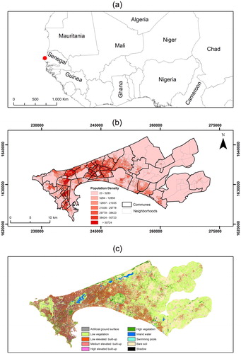
Dakar is the capital of Senegal, located in the westernmost part of the African continent. The climate is typically Sahelian with a humid season extending over the summer months and until November and a longer, dry season in the rest of the year. According to the latest data, the city of Dakar has roughly 1.14 million inhabitants, while the extended, metropolitan region of Dakar (including peri-urban areas) contains about 3 million residents (Agence Nationale de la Statistique et de la Démographie 2013). Dakar is a major economic center and has been undergoing rapid urbanization in the last decades. This has led to increasing health and socio-economic inequalities and the growth/creation of informal/deprived settlements in the region (Borderon 2013). Since population information at a fine scale are very rare for several SSA cities, we selected Dakar as a case study because of the existence of detailed population information as well as a whole set of ancillary information that are available for the city such as very-high-resolution LC and LU maps.

Dataset

As the dependent variable, we use the population density of the recent 2013 census at the neighbourhood level provided by the National Agency for Statistics and Demography of Senegal (Agence Nationale de la Statistique et de la Démographie 2013). The national census database provides population data with three residential conditions: present, absent and visitors. The latter are not part of the household in which they are counted and were excluded in the population calculation to avoid double counting. The neighbourhood is the smallest administrative (level 5) unit in Dakar. The total number of training units is 1319 (clipped to match the extent of the RS datasets) while each one of them belongs to one of the 52 administrative communes of Dakar (Figure 1). Due to the highly skewed distribution of the population density, we use a log transformation as frequently done in population prediction studies (Linard et al. 2013; Stevens et al. 2015). We extract independent variables from an open access LC classification of Dakar derived from a 2015 VHR Pleiades (0.5 meter) satellite imagery based on the extent of the population map (Grippa and Georganos 2018; Figure 1c). The LC map has been recently used as reference in recent population, land-use and urban climate studies in Dakar (Grippa et al. 2018, 2019; Brousse et al. 2019) due to its high quality, scoring 89.5% on overall map accuracy and 94% on the F-score for the buildings class. Finally, we operate under the assumption that the 2-year temporal gap between the Pleiades imagery and the census is negligible.

Figure 1. (a) Location map of Dakar within the African continent, (b) Population density at the neighbourhood administrative level in Dakar, Senegal. The independent variable used in the models was the logarithmic transformation of the population density values due to the skewness of the distribution. (c) Land cover map of Dakar at a 0.5 m resolution.

Afterwards, we selected four approaches to model population as a function of RS covariates, i) using all available LC classes and geographic coordinates simultaneously (LC_XY), ii) using only LC classes (LC), iii) using the three built-up LC classes and geographic coordinates (3BU_XY) and iv) using only the three built-up classes (3BU; Table 1). Including geographical coordinates as explanatory features aims to account for potential spatial dependency as shown recently and is recommended as a good practice when working with spatial data (Hengl et al. 2018). For each neighbourhood, we extracted the proportions of the LC classes. As an illustrative example, Figure 2 visualizes the proportions of three land cover classes (low elevated buildings, trees and inland water). Finally, for evaluating the results of our methods we sample 5 communal units (168 neighbourhoods) which correspond to roughly 10% of the total spatial units while the rest of the data are used for training. The rationale for sampling communal units instead of neighbourhoods is to maintain spatial independency of the out-of-sample validation set and ensure unbiased conclusions.

Figure 2. Examples of independent variables used in the study. Proportions of (a) low elevated built up (<5 meters), (b) high vegetation and (c) inland water.

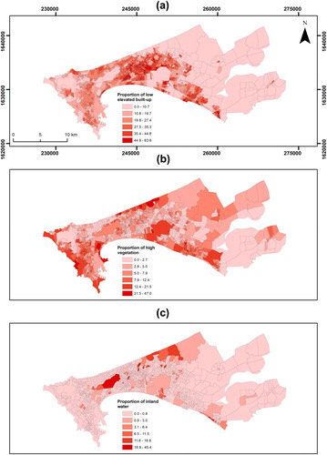
Table 1. Independent variables and models used in the analysis.

Variable	LC_XY	LC	3BU_XY	3BU
Low elevated built-up (<5 m)	✔	✔	✔	✔
Medium elevated built-up (5–10 m)	✔	✔	✔	✔
High elevated built-up (>10 m)	✔	✔	✔	✔
Bare ground	✔	✔
Low vegetation	✔	✔
High vegetation	✔	✔
Shadows	✔	✔
Inland water	✔	✔
XY coordinates	✔		✔

Population modelling

Random forest

RF is an aggregation of several Classification and Regression Trees (CARTs) (Breiman 2001). They were developed to combat important limitations of using a single CART such as overfitting. Breiman (2001) suggested that by combining the predictions of several independent CARTs and adding bagging in the process the generalization of the model would be superior, which is often the case. In the traditional RF formulation, each decision tree is randomly created by sampling roughly two-thirds of the training data with replacement while the other third is kept out of training (training data bagging). Moreover, while building each tree, only a random subset of features is selected at each decision node (feature bagging). In the end, the majority vote (classification) or the average predictions of all trees (regression) is used to create the final output – the forest. At the same time, the third of the data that is kept out on each tree can be used for computing a performance evaluation metric, the Out of Bag (OOB) error estimate (Breiman 2001). By using the OOB error, the importance of the independent variables can be assessed. The most popular way to do so is by using the increase in the Mean Squared Error (iMSE). In detail, the values of each feature are randomly permuted and the OOB error iMSE is computed. We compare that value with the original model performance before the permutation and hence, if a variable is very important, we expect a large increase in the OOB error and vice versa. The salient parameters of the RF are the number of trees to grow and the number of randomly selected independent variables on each split during the development of each tree. The former is set as high as computationally efficient with most RS applications ranging between 200 and 500 while the latter is determined through minimization of the OOB error (Pal 2005).

Geographical random forest

RF is still a global and ‘aspatial’ concept that might not address spatial heterogeneity. As such, we extend RF as a disaggregation consisting of several local sub-models. The principle idea is similar to that of GWR (Fotheringham et al. 2003), in which we move to local computation rather than global one. This means that for each location i, a local RF is computed but only including a n number of nearby observations. Essentially, this leads to the calculation of an RF in each training data point, with its own performance, predictive power and feature importance. In that way, we increase the flexibility of RF to be calibrated locally rather than globally. To describe the difference between the two methods, we use a simplistic version of a regression equation: (1) $$Y_i= a{x}_i+ e,i = 1: n$$(1) where Y_i is the value of the dependent variable for the ith observation and ax_i is the non-linear prediction of RF based on a set of x independent variables, with e being an error term. The above equation is formed by using all the data at the same time, disregarding their spatial distribution. In GRF, we extend Equation (1)(1) $$Y_i= a{x}_i+ e,i = 1: n$$(1) : (2) $$Y_i= a\left(u_i, v_i\right)x_i+ e,i = 1: n$$(2) where a(u_i, v_i)x is the prediction of an RF model calibrated on location i, and (u_i, v_i) are the coordinates. A sub-model is built for each data location, considering only nearby observations. The area that the sub-model operates in is called the neighbourhood (or kernel), and the maximum distance between a data point and its kernel is called the bandwidth (Brunsdon et al. 1998). There are two usual types of kernels, ‘adaptive’ and ‘fixed’ (Kalogirou 2015). In the former, the neighbourhood is defined by n nearest neighbours and in the latter, by a circle whose radius is the bandwidth (Brunsdon et al. 1998; Fotheringham et al. 2003). In this study, we employ an adaptive kernel and we investigate results with several numbers of n. Using an adaptive kernel is advantageous when sampling density is different across space – which is the case in our dataset, as the census units can vary dramatically in size. For predicting, we fuse the global and local estimates using a weight parameter (a). Fusing the predictions allows us to extract the locally heterogeneous signal (low bias) from the local sub-model and merging it to that of a global model which uses more data (low variance). The weight parameter can be user defined and for the scopes of this study we experimented with three settings i) a = 0.25 which implies less weighting for the local model in favour of the global one, ii) a = 0.50 which means equal weighting for the local and global models and iii) a = 0.75 which implies a favourable weighting for the local model. To predict on new spatial locations, the closest available GRF model is used. To implement the GRF and RF analyses, we used the recently developed R package ‘SpatialML’ (Kalogirou and Georganos 2018).

Ultimately, GRF can be used for two aims: i) improve predictions over a traditional RF and ii) extract spatially differentiated inferences of model parameters. For the former, the improvement in performance is a function of appropriate bandwidth selection and the degree of spatial heterogeneity in the data. For the latter, it can be used as an easily applied tool to explore the local structure of the data and enhance our understanding of how geographical processes operate on them. Since the sub-models are calibrated locally, the outputs of GRF can be fully visualized as maps that illustrate the spatial interaction among variables but also highlighting areas of interest that are not possible to detect through global models.

Model evaluation

To evaluate the accuracy of the models we employ two established and robust error measurement metrics, Root Mean Squared Error (RMSE; Equation (3)(3) $$\mathrm{RMSE}=\mathrm{ }\sqrt{\frac{\sum _{i=1}^n{(y_i-x_i)}^2}{n}}$$(3) ) and Mean Absolute Error (MAE; Equation (4)(4) $$\mathrm{MAE}=\mathrm{ }\frac{{\sum }_{i=1}^n\left|y_i-x_i\right|}{n}$$(4) ): (3) $$\mathrm{RMSE}=\mathrm{ }\sqrt{\frac{\sum _{i=1}^n{(y_i-x_i)}^2}{n}}$$(3) (4) $$\mathrm{MAE}=\mathrm{ }\frac{{\sum }_{i=1}^n\left|y_i-x_i\right|}{n}$$(4) where x_i is the observed variable, y_i is the predicted value, and n is the sample size.

Another way to assess the quality of a model applied on geographical data is that degree of residual spatial autocorrelation (RSA). A high degree of RSA violates spatial regression assumptions concerning the independence of observations. To investigate this, we employ the commonly used Moran’s I Index (MI) (Moran 1948; Anselin 2010; Equation (5)(5) $$MI=\frac{n{\sum }_i^{}{\sum }_j^{}{w}_{\mathit{ij}}{z}_i{z}_j}{M\sum _{i=1}^n{z}_i^2},$$(5) ) to assess the level of residual autocorrelation in incrementally increasing distance ranges. 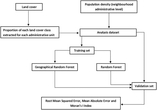(5) $$MI=\frac{n{\sum }_i^{}{\sum }_j^{}{w}_{\mathit{ij}}{z}_i{z}_j}{M\sum _{i=1}^n{z}_i^2},$$(5) where n is the number of data points, z_i = x_i − $\overline{x},$ $\overline{x}$ is the mean value of x, M = ${\sum }_{i=1}^n{\sum }_{j=1}^n{w}_{\mathit{ij}}$ and w_ij is the element of the matrix of spatial proximity M, which depicts the degree of spatial association between the points i and j (Kalogirou and Hatzichristos 2007). The MI value range is between −1 and 1 with values larger than 0 implying positive spatial autocorrelation. Finally, the methodological workflow is briefly summarized in the flowchart of Figure 3.

Figure 3. Flowchart depicting the methodological framework.

Results

Measuring the effect of geographic scale and weight parameter

An important facet of investigation is the scale effects on the performance of GRF. To do so, we compare the MAE and RMSE against GRF’s with bandwidths of different n (number of nearest observations) and different weight parameters. In Figures 4 and 5, we present the results for RMSE and MAE, respectively. As shown in the figures, it is evident that there is a pattern in the distribution of RMSE and MAE as a function of the bandwidth and weight parameter specified, irrespective of the model used.

Figure 4. RMSE of GRF with incrementing bandwidth (number of nearest neighbours) using proportions of (a) all LC classes and geographical coordinates as explanatory factors, (b) all LC classes, (c) 3 types of built-up and geographical coordinates and (d) 3 types of built-up as input. The last point in each graph represents the global RF model.

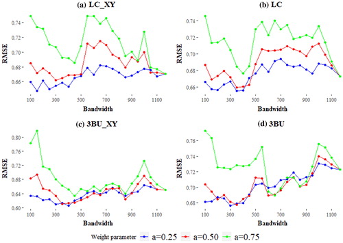
Figure 5. MAE of GRF with incrementing bandwidth (number of nearest neighbours) using proportions of (a) all LC classes and geographical coordinates as explanatory factors, (b) all LC classes, (c) 3 types of built-up and geographical coordinates and (d) 3 types of built-up as input. The last point in each graph represents the global RF model.

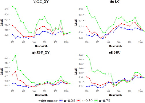
In all four modelling designs, it appears that weighting the local predictions too heavily (a = 0.75) is suboptimal in terms of accuracy and in most cases, even a global RF model would perform similarly or better. On the contrary, when using moderate or lighter weights for the fusion (a = 0.50 and 0.25) the GRF may produce better predictions, especially in a certain range of bandwidths. In particular, the bandwidth range between 100 and 400 systematically exhibits the lowest RMSE and MAE values in all four approaches. Weight values of 0.25 for the LC and LC_XY models and 0.25–0.50 for the 3BU and 3BU_XU approaches are the most optimal choices in terms of minimizing RMSE and MAE and consistently predict better than a global RF. Finally, defining a GRF with small bandwidths (<200) appears to create unstable models with very high MAE and RMSE values.

Notably, there are differences in the results, not only within each modelling approach but also among them (i.e. 3BU vs LC). Using only the built-up classes and geographical coordinates (3BU_XY) produced the most accurate global and local models (Table 2). Interestingly, the gap in performance between GRF and RF was highest when training with the 3BU_XY input. Considering all different parameters and inputs, the best performing method was that of the 3BU_XY GRF, with a weight parameter of 0.25, and a bandwidth of 400 (RMSE = 0.606, MAE = 0.421) with its global counterpart (3BU_XY RF) underperforming (RMSE = 0.650, MAE = 0.453). In all cases, the differences between the predictions of the best performing GRFs and RFs were significant using a paired t-test (p < 0.05). Finally, in all cases but the first (LC_XY), the optimal bandwidths minimizing RMSE and MAE were the same or very similar (bandwidth = 350–400; Table 2).

Table 2. RMSE and MAE of the most accurate GRF against the global model.

Model	RMSE bandwidth	GRF RMSE	Global RMSE	MAE bandwidth	GRF MAE	Global MAE	Weight
LC_XY	150	0.648	0.671	400	0.467	0.489	0.25
LC	350	0.656	0.673	400	0.478	0.503
3BU_XY	400	0.606	0.650	400	0.421	0.453
3BU	300	0.677	0.723	350	0.514	0.557

Residual spatial autocorrelation

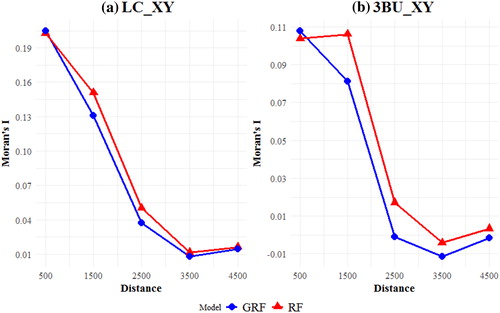
High RSA is a typical phenomenon when a model has not been specified correctly, usually by missing important explanatory variables or by failing to account for spatial dependency or heterogeneity. In this example, we investigate the degree of RSA by calculating MI at incrementing spatial scales for RF and GRF on the validation dataset. We investigate RSA in the predictions of the two best performing models (3BU_XY and LC_XY). Irrespective of the type of modelling approach, GRF residuals systematically exhibit lower MI values (Figure 6). In both cases, RSA usually weakens as we increase the distance lags. Notably, RSA is considerably lower when only built-up classes are used, which complements the results of RMSE and MAE above.

Figure 6. Moran’s I Index for GRF AND RF at incrementing spatial lags with two different training inputs. (a) LC_XY and (b) 3BU_XY.

Visualising GRF

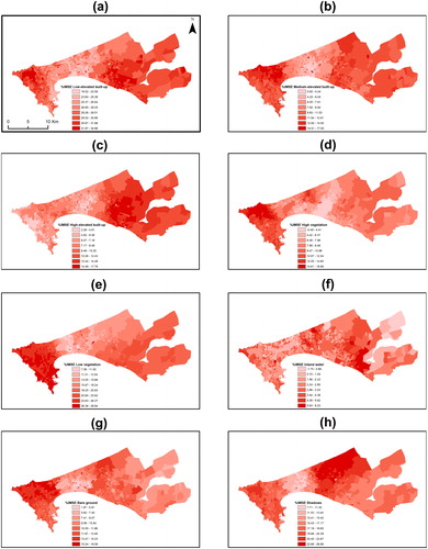
GRF can also be used as a purely exploratory tool rather than a predictive one. GRF is a local decomposition of the RF and hence, the results can be mapped. Using the whole dataset without training/testing splits (for better visualization) and a bandwidth of 400 neighbours, the distribution of the performance of the local models is illustrated (Figure 7). The local models are stronger (pseudo-R² > 0.6) in the peri-urban zones (Rufisque) while they become less accurate (pseudo-R² < 0.5) in the dense and small-sized administrative neighborhoods of western Pikine and the large, industrial areas of southeast Dakar. The latter suggests that in these regions, additional variables should be included to further improve the performance of the models. Moreover, the spatial variation of the importance of each independent variable can also be illustrated (Figure 8), which is presented in the form of in iMSE. Notably, there is a strong degree of spatial interaction between each predictor while the importance of each predictor varies dramatically through space. Interestingly, all three built-up variables seem to be less important in Pikine. Moreover, the two vegetation types (low and high vegetation) appear to be strongly more predictive over the city of Dakar and less important on the extending metropolitan region. Similarly, the rest of the predictive variables formulate unique spatial patterns.

Figure 7. Pseudo-local coefficient of determination of GRF. Higher values indicate better performance while low values may imply missing variables or inadequate input data.

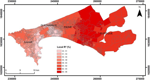
Figure 8. Examples of local feature importance of independent variables by using the iMSE. Higher values imply increased importance. (a) Low elevated built-up, (b) medium elevated built-up, (c) high elevated built-up, (d) high vegetation, (e) low vegetation, (f) inland water, (g) bare ground and (h) shadow.

Computational performance

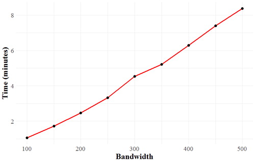
The current GRF implementation is single-thread only. In Figure 9, the computational time against different bandwidths is illustrated. GRF models calibrated with small numbers of neighbours are relatively fast but without a doubt, the local implementation can be significantly more computationally tedious than a global RF. In the current dataset, using all covariates (LC_XY) and specifying 400 neighbours, GRF required 6.29 minutes to run while RF only 2.3 seconds.

Figure 9. Computational burden of GRF.

Discussion

GRF as a predictive and exploratory tool

The first empirical results from the application of GRF are encouraging on its use as both a predictive and exploratory tool. We demonstrate that by selecting an appropriate geographic scale to analyse the data, GRF can outperform a globally specified RF with more accurate predictions and lower RSA. This geographic scale can be described as the operational scale of the relationship which includes just enough data points to capture the inherent localities while at the same time rejecting/reducing unnecessary training data that come from locations afar, that might be considered as noise to the model (Propastin 2009; Gao et al. 2012). On the contrary, using bandwidths defined with a very small number of neighbours can provide discouraging results. This can be explained by the use of very few training data points to calibrate the local models in an appropriate manner. Finally, including the geographical coordinates as features appears to be a good practice when using ML algorithms with spatial data, confirming prior research (Hengl et al. 2018). Since RF is a decision tree (DT) algorithm, using explicitly spatial features such as coordinates can enforce a degree of spatial interaction in the development of the trees and -at least partly- address spatial non-stationarity.

The results are in accordance with previous studies that have investigated spatial non-stationarity in linear models and population prediction (Cockx and Canters 2015). Even though RF is a highly flexible and non-linear algorithm, it is inevitably a model which may not account for spatial heterogeneity. Moreover, it can be quite challenging to identify and address spatial heterogeneity in ML models as they are not based on strict parametric distributions such as generalized linear models. As a helping hand, GRF can illustrate these effects in a very practical way along with a set of other information such as the local performance of the independent variables. Nonetheless, this information comes with an important limitation - increased computational complexity.

In this application, the results were very straightforward – the optimal performance of GRF is a function of an appropriate bandwidth and weight parameter selection. Nonetheless, according to different datasets the results may be different. For example, in cases with very high degrees of spatial heterogeneity, weighting the local component more could provide more robust estimates and vice-versa.

Future research prospects

As mentioned previously, the current implementation is single-thread and may cost considerable time to compute the GRF. Nonetheless, this issue can be mitigated by parallelizing the procedure, a feasible task since the computation of local sub-models can be happen simultaneously as they are independent. Additionally, GRF uses the randomForest R package (Liaw, Wiener 2002) to implement GRF. Nonetheless, there exist other RF implementations that are significantly faster such as the ranger R package and should be explored. Moreover, ranger allows for setting weights for each observation and therefore a more geographic weighting of the training data points can be applied. For example, as in the latest GWR implementations (Fotheringham et al. 2015), training data points closer to a specific spatial or temporal location can be weighted as more important than those further away. Another topic we have to be cautious about is the use of GRF as a strictly predictive tool. As in GWR, tests that justify its use should be developed. One way to do so is to investigate if there is enough spatial variation in the local feature importance of each predictor to justify its use (Osborne et al. 2007).

An additional topic for future research relates to local parameter fine-tuning and local feature selection. In the current implementation, GRF assumes a homogeneous parametrization across each local sub-model. This is true for the parameters of RF such as the number of trees and number of splits in each node but also for the number of predictors used as input. A more sophisticated implementation would entail different parameter tuning in each sub-model coupled with local feature selection. As shown in the results, providing only the least noisy features can reduce the error of the prediction and it would be reasonable to hypothesize that a variable could be selected in a local context but not a global one. One way to do this would be to apply simple and efficient feature selection procedures before computing a local model with algorithms such as Variable Selection Using Random Forest (VSURF; Genuer et al., 2015) and Recursive Feature Elimination (RFE; Georganos et al., 2017b; Ma et al., 2017).

Finally, other ML algorithms should be evaluated for a geographical implementation. Although this study uses the RF algorithm as an example, other ML algorithms such as Support Vector Machines (SVM) and Boosting Regression Trees (BRT) might be better candidates according to different datasets and requirements. For example, SVM is orders of magnitude faster than regression trees and thus can be a solid alternative in the face of limited computational power while BRT are very strong from a prediction perspective if their parameters are fine-tuned well enough.

Conclusions

In this study, we introduce a local version of the RF algorithm for geographical data, named GRF. We introduce GRF for modelling population as a function of very-high-resolution remotely sensed land cover data. The empirical results of this first application demonstrate the twofold use of GRF for i) improving the accuracy of the predictions against a traditional RF and ii) exploring and visualizing the spatial structure of RF as a decomposition of local sub-models. For the former, identifying the appropriate spatial scale to model the relationship between independent and dependent variables was the most important factor to achieve better predictions. Moreover, a crucial component is to select a suitable weight parameter when fusing the local and global estimates as the output of GRF. With respect to the latter, GRF can be deployed as an easy to use tool for investigating spatial variations in model performance and feature importance, highlighting potentially interesting variations that are constrained in the use of RF.

Disclosure statement

No potential conflict of interest was reported by the authors.

Additional information

Funding

This research was funded by BELSPO (Belgian Federal Science Policy Office) in the frame of the STEREO III program, as part of the MAUPP (SR/00/304) and REACT (SR/00/337) project (http://maupp.ulb.ac.be and http://react.ulb.be/). The population data were provided by the ASSESS project, funded by the ARES-CDD.

References

- Agence Nationale de la Statistique et de la Démographie (ANSD). 2013. Rapport Définitf Du RGPHAE 2013. Dakar, Senegal.
- Amaral S, Monteiro AMV, Camara G, Quintanilha JA. 2006. DMSP/OLS night-time light imagery for urban population estimates in the Brazilian Amazon. Int J Remote Sens. 27(5):855–870.
- Anselin L. 2010. Lagrange multiplier test diagnostics for spatial dependence and spatial heterogeneity. Geogr Anal. 20(1):1–17.
- Borderon M. 2013. Why here and not there? Developing a spatial risk model for malaria in Dakar, Senegal. From social vulnerability to resilience: measuring progress toward disaster risk reduction; p. 108–120.
- Breiman L. 2001. Random forests. Machine Learn. 45(1):5–32.
- Brousse O, Georganos S, Demuzere M, Vanhuysse S, Wouters H, Wolff E, Linard C, Nicole P-M, Dujardin S. 2019. Using local climate zones in sub-saharan Africa to tackle urban health issues. Urban Clim. 27:227–242.
- Brunsdon C, Fotheringham S, Charlton M. 1998. Geographically weighted regression. J Royal Stat Soc D. 47(3):431–443.
- Cockx K, Canters F. 2015. Incorporating spatial non-stationarity to improve dasymetric mapping of population. Appl Geogr. 63:220–230.
- Foody GM. 2003. Geographical weighting as a further refinement to regression modelling: an example focused on the NDVI–rainfall relationship. Remote Sens Environ. 88(3):283–293.
- Fotheringham AS, Brunsdon C, Charlton M. 2003. Geographically weighted regression: the analysis of spatially varying relationships. Hoboken, NJ: John Wiley & Sons.
- Fotheringham AS, Crespo R, Yao J. 2015. Geographical and temporal weighted regression (GTWR). Geogr Anal. 47(4):431–452.
- Fotheringham AS, Yang W, Kang W. 2017. Multiscale geographically weighted regression (MGWR). Ann Am Assoc Geogr. 107(6):1247–1265.
- Gao Y, Huang J, Li S, Li S. 2012. Spatial pattern of non-stationarity and scale-dependent relationships between NDVI and climatic factors—a case study in Qinghai-Tibet Plateau, China. Ecol Indic. 20:170–176.
- Genuer R, Poggi J-M, Tuleau-Malot C. 2015. VSURF: an R package for variable selection using random forests. R Journal. 7(2):19–33.
- Georganos S, Abdi AM, Tenenbaum DE, Kalogirou S. 2017a. Examining the NDVI-rainfall relationship in the semi-arid Sahel using geographically weighted regression. J Arid Environ. 146:64–74.
- Georganos S, Grippa T, Vanhuysse S, Lennert M, Shimoni M, Kalogirou S, Wolff E. 2017b. Less is more: optimizing classification performance through feature selection in a very-high-resolution remote sensing object-based urban application. GISci Remote Sens 55:221–242.
- Grippa T, Georganos S. 2018. Dakar very-high resolution land cover map. Zenodo repository. Available from: https://zenodo.org/record/1290800#.XLbiKOgzY2w
- Grippa T, Georganos S, Zarougui S, Bognounou P, Diboulo E, Forget Y, Lennert M, Vanhuysse S, Mboga N, Wolff E. 2018. Mapping urban land use at street block level using OpenStreetMap, remote sensing data, and spatial metrics. ISPRS Int J Geo-Inf. 7(7):246.
- Grippa, T, Linard, C, Lennert, M, Georganos, S, Mboga, N, Vanhuysse, S, Gadiaga, A, Wolff, E. 2019. Improving urban population distribution models with very-high resolution satellite information. Data. 4(1):13.
- Hengl T, Nussbaum M, Wright MN, Heuvelink GBM, Gräler B. 2018. Random forest as a generic framework for predictive modeling of spatial and spatio-temporal variables. PeerJ. 6:e5518.
- Kalogirou S. 2015. Destination choice of athenians: an application of geographically weighted versions of standard and zero inflated poisson spatial interaction models. Geogr Anal. 48(2):191–230.
- Kalogirou S, Georganos S. 2018. “SpatialML.” R Foundation for Statistical Computing.
- Kalogirou S, Hatzichristos T. 2007. A spatial modelling framework for income estimation. Spatial Econ Anal. 2(3):297–316.
- Laros M, Jones F. 2014. “The State of African Cities 2014: re-imagining sustainable urban transitions.”
- Liaw A, Wiener M. 2002. Classification and Regression by randomForest. R News. 2(3):18–22.
- Linard C, Tatem AJ, Gilbert M. 2013. Modelling spatial patterns of urban growth in Africa. Appl Geogr. 44:23–32.
- Liu X, Clarke K, Herold M. 2006. Population density and image texture. Photogramm Eng Remote Sens. 72(2):187–196.
- Lo CP. 2008. Population estimation using geographically weighted regression. GISci Remote Sens. 45(2):131–148.
- Ma L, Fu T, Blaschke T, Li M, Tiede D, Zhou Z, Ma X, Chen D. 2017. Evaluation of feature selection methods for object-based land cover mapping of unmanned aerial vehicle imagery using random forest and support vector machine classifiers. ISPRS Int J Geo-Inf. 6(2):51.
- Moran PAP. 1948. The interpretation of statistical maps. J R Stat Soc. B Methodol. 10(2):243–251.
- Osborne PE, Foody GM, Suárez-Seoane S. 2007. Non-stationarity and local approaches to modelling the distributions of wildlife. Divers Distrib. 13(3):313–323.
- Pal M. 2005. Random forest classifier for remote sensing classification. Int J Remote Sens. 26(1):217–222.
- Propastin PA. 2009. Spatial non-stationarity and scale-dependency of prediction accuracy in the remote estimation of LAI over a tropical rainforest in Sulawesi, Indonesia. Remote Sens Environ. 113(10):2234–2242.
- Stevens FR, Gaughan AE, Linard C, Tatem AJ. 2015. Disaggregating census data for population mapping using random forests with remotely-sensed and ancillary data. PLoS One. 10(2):1–22.
- UN Desa. 2018. World urbanization prospects, the 2018 revision. Population Division, Department of Economic and Social Affairs, United Nations Secretariat.
- Wu C, Murray AT. 2007. Population estimation using landsat enhanced thematic mapper imagery. Geogr Anal. 39(1):26–43.
- Wu S-S, Qiu X, Wang L. 2005. Population estimation methods in GIS and remote sensing: a review. GISci Remote Sens. 42(1):80–96.