Water quality spatial-temporal analysis of gravel pit ponds in the southeast regional park Madrid (Spain) from 1984 to 2009.

Abstract

We used a time series of Secchi disk values retrieved from Landsat 5 images to study temporal and spatial patterns of water quality across gravel pit ponds located in Madrid, Spain from 1984 to 2009. There is a seasonal behavior in the water quality, with higher values of Secchi disks in autumn and winter (December–February) and lower values in summer (July–August), which can be explained by the relationship between Secchi disk values and temperature and solar radiation. We found that the 1994 administrative declaration of the regional park has had a positive impact on the water quality. The trophic state of the studied pit ponds has slowly improved, though the ponds have not reached the oligotrophic state.

Keywords:

• Inland water
• Secchi depth
• transparency
• spatial–temporal series
• gravel pit pond

Introduction

Sand and gravel are fundamental to the development of the urban and industrial economy (construction, civil works, and infrastructure) (Mollema and Antonellini 2016; Søndergaard et al. 2018; U.S. Geological Survey 2015). The most intensely exploited deposits are typically very close to large cities, which are the main consuming centers of these materials (Vucic et al. 2019). Spain (along with Italy) had the highest rates of urban growth of the future European Union in the 1960s. During that decade and the next, nine of the twelve European urban agglomerations with the most growth were Spanish, with Madrid taking the lead (Díaz and Araujo 2017). This activity has resulted in the generation of gravel ponds due to the rise of the phreatic level when dredging was carried out. When abandoned, these ponds and artificial lakes became wetland ecosystems with established aquatic fauna and flora (Domínguez Gómez and Peña 1999). This phenomenon is common across the world. For example, in Maine, USA, 34 active and former gravel pits cover 26% of the aquifer surface (Peckenham et al. 2009); in the Netherlands, 500 gravel pit lakes give this country the highest production of gravel and sand per surface area of all countries (Mollema et al. 2015); in Italy, the gravel pit lakes along the coast near Ravenna increased the open water surface in the catchment by 6% from 1972 to 2012, and the excavation is not yet finished (Mollema et al. 2012); in Nottinghamshire, UK, gravel pits exploited between 1929 and 1967 became the Attenborough Nature Reserve and received the designation of a Site of Special Scientific Interest (SSSI) (Andrews 1990).

In recent years, interest in protecting the environment that hosts this type of extractive activity has increased. This is the case in Madrid. In 1994, the declaration of the regional park ‘Parque Regional del Sureste’ (PRSE) (Ley 6/1994, Spain) was made in order to protect the area of the Manzanares and Jarama rivers’ confluence, including the gravel pit ponds, against all kinds of negative environmental impacts.

The gravel pit ponds are peculiar water bodies. They are young compared to most natural lakes, given that they are less than one hundred years old; dynamic due to their origin; and difficult to access because they are on private property. As a result, it has not been possible to investigate long-term environmental concerns for these ponds, and they have not been studied in detail compared to other types of natural and man-made lakes (Vucic et al. 2019). Thus, it is necessary to study gravel pit lakes’ water quality, their aquatic ecosystem function, and the effects of environmental changes (Mollema and Antonellini 2016). Such research is important both due to its ecological importance and because this type of wetland will continue to be generated in metropolitan areas such as Madrid, given that urban development is continuous.

Since the 1980s, there has been a high level of interest in the gravel pit ponds in the PRSE, which have consequently been widely studied through field campaigns (Álvarez-Cobelas 1991; Álvarez-Cobelas et al. 1987; Álvarez-Cobelas 2000). However, the conservation status of the lentic ecosystems located in the PRSE has not been periodically monitored. Such monitoring is essential because the role of wetland ecosystems, as well as how that role will change with increasing pressure from human activity and climate change, require significant study (Álvarez-Cobelas et al. 2019).

Several national and international directives address these problems and aim to improve the ecological state of inland waters. In EU Member States, the Water Framework Directive (WFD) was intended to unify water management efforts in the European Union. Since its approval, the European Communities have the responsibility of monitoring the water quality of their waterbodies (EC 2000). However, for a comprehensive understanding of lake ecology, integrative, frequent, and consistent long-term monitoring approaches are required (Hestir et al. 2015; Seelen et al. 2021). Understanding the temporal trends and spatial distributions of water quality is essential for maintaining the health of aquatic ecosystems and ensuring the safety of water (Blanchet et al. 2022; Chu et al. 2018). To this end, spatio-temporal modeling for water quality has produced considerable advances over the last few decades (Kim et al. 2017; Kim et al. 2015; Liu et al. 2021; Seers and Shears 2015; Weeks et al. 2012; Yoder et al. 2002).

Remote sensing is a highly useful tool to achieve this aim. Global mapping satellite missions make systematic measurements over years or decades, providing a time series of consistently measured data to assess system conditions, identify changes and understand processes for an important suite of biophysical variables. Even if monitoring is generally performed using field data, remote sensing can play a key role as it offers the opportunity to extend monitoring at low cost (Devlin et al. 2015; el Serafy et al., 2021) and examine the spatial and temporal variability of water quality data (Boucher et al. 2018; Chao Rodríguez et al. 2014; Domínguez Gómez et al. 2009; Hicks et al. 2013; Li et al. 2021; Lobo et al. 2021; López-Andreu et al. 2021; Maeda et al. 2019; Nas et al. 2010; Paltsev and Creed 2021; Wang et al. 2021).

In a previous study, transparency measured by Secchi disk (SD) values was obtained for the PRSE water bodies from 1984 to 2009 using a regression equation that relates field data and the reflectance of the Landsat 5 image. This method produced a spatial–temporal series of SD data (Echavarría-Caballero et al. 2019).

These time series can be approached by predictive modeling (Delasalles et al. 2019) or exploratory analysis (Cressie and Wikle 2015). In the latter case, methods such as the Hovmöller diagram, anomalies analysis, and the empirical orthogonal function (EOF) have a long history of being used in remote sensing to study atmospheric phenomena (Hannachi et al. 2007; Liew et al. 2010; Persson 2017). More recently, they have been used in water studies (Beltrán-Abaunza et al. 2017; Bracher et al. 2020; Weeks et al. 2012; Yoder et al. 2002)

Spatial–temporal SD data provides an opportunity to better understand the behavior of water quality in gravel pit ponds. Therefore, the aim of our research is to carry out statistical analysis in order to assess the spatial and temporal patterns of water quality using time series of SD data retrieved from Landsat 5 images. In particular, we aimed to (1) detect changes and magnitudes of the differences in water transparency in space and time; (2) characterize the seasonal behavior of SD; and (3) determine the dominant modes of variation and identify the physical drivers that influence the spatio-temporal patterns of water transparency.

Study area

The study focuses on the PRSE (Figure 1), which covers an area of 300 km² in 18 municipalities located in the southwestern part of the Madrid region (Spain). The area includes the lower course of the Jarama River, specifically from Coslada to Aranjuez-Ciempozuelos.

Figure 1. Study area, including gravel pit ponds (bright blue) and the boundary of the PRSE (black).

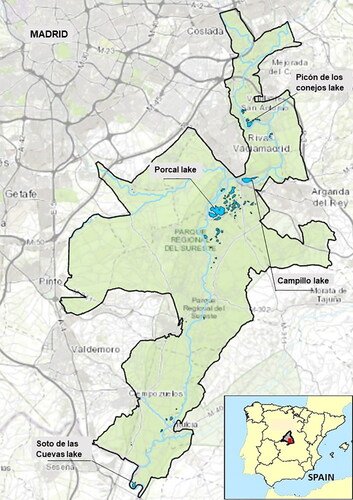
The PRSE is characterized by the presence of two fundamental lithological domains: the Neogene Tertiary and the Quaternary. It is included in the Tajo basin, specifically in the sub-basin belonging to the Jarama River. This river is the main watercourse in the park and runs in the north–south direction (Moreno & García-Avilés, 1997; Mostaza-Colado et al. 2018). The flora includes primarily helophyte vegetation, especially reeds (Phragmites australis), accompanied by bulrushes (Typha spp.), rushes (Scirpus holoschoenus), and repopulations of native species such as alders, poplars, and elms, as well as more exotic species such as tree of paradise and weeping willow (Moreno & García-Avilés, 1997). The climate in the study area is classified as Mediterranean temperate-continental, with temperate winters and warm, dry summers. The average temperature is 13.8 °C and the average rainfall is 440 mm/year (Mostaza-Colado et al. 2018).

In the environment of the PRSE, water is the omnipresent and dominant natural element. Rivers and lakes have shaped the territory of the park and support a large number of species. In the PRSE, a total of 123 wetlands have been inventoried, occupying more than 400 hectares. To develop the current research, we selected four gravel pit ponds: Picón de los Conejos, Campillo, Porcal, and Soto de las Cuevas. We applied three selection criteria, choosing water bodies (1) with sufficient size to be analyzed according to the spatial resolution of the Landsat 5 images; (2) that are distributed throughout the study area and (3) that belong to areas with different environmental classifications (degraded zones for regeneration, conservation areas and orderly exploitation of natural resources zones). The water bodies developed by gravel extraction, which are the subject of this study, will be named as gravel pit ponds, gravel pit lakes, water bodies, or lakes.

Picón de los Conejos gravel pit pond

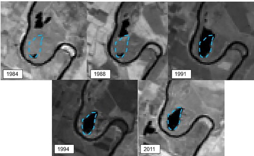
The Picón de los Conejos gravel pit pond complex originated in 1991 and comprises four water bodies. It underwent multiple transformations until 1994, when it stabilized in its current form (Figure 2). For the purposes of the present study, the analysis of water quality in this pond has been carried out since 1994.

Figure 2. Picón de los Conejos lake development from 1987 to 2011, with the assumed shape in this study (light blue dashed line).

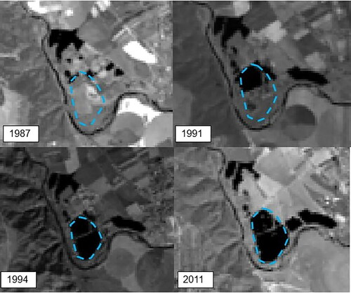
According to the environmental park zoning developed in the Planning and Management Plan in Protected Natural Areas (Decreto 27/1999 of February 11th, Madrid), the Picón de los Conejos gravel pit pond complex is located in zone C, which corresponds to the degraded zones for regeneration classification. It has been included in the ‘cataloged wetlands’ by the Madrid regional government given its unique landscape, fauna, botany, hydrological, ecological, or geological characteristics (Comunidad de Madrid 2020).

Campillo gravel pit pond

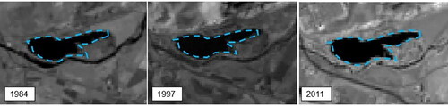
As this lake maintained its extension throughout the study period, its water quality is evaluated from 1984 to 2009 (Figure 3). According to the zoning of the regional park, the Campillo lake is located in zone B, which is conservation zone. It has been included in the ‘cataloged wetlands’ by the Madrid regional government.

Figure 3. Campillo lake development from 1984 to 2011, with the assumed shape in this study (light blue dashed line).

The Porcal gravel pit pond

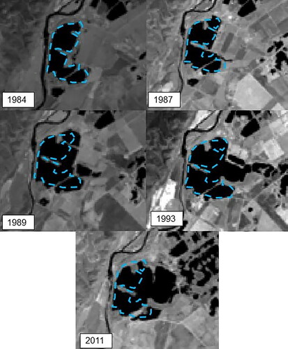
The Porcal lake has undergone changes throughout the time series of the present study (from 1984 to 2011). Therefore, the water quality study of this water body is only carried out in the area formed since 1984 (dashed blue line in Figure 4). Porcal lake is located in zone D, orderly exploitation of natural resources, according to the zoning of the regional park.

Figure 4. Porcal lake development from 1984 to 2011, with the assumed shape in this research (light blue dashed line).

Soto de las Cuevas

Soto de las Cuevas lake was partially formed in 1984, but it was not until 1991 that it reached its current form (Figure 5). Therefore, the water quality study of this lake has been carried out since 1991. According to the zoning of the regional park, the Soto de las Cuevas lake is located in zone B, conservation area, and it is included in the ‘cataloged wetlands’ by the Madrid regional government.

Figure 5. Soto de las Cuevas lake development from 1984 to 2011, with the assumed shape in this research (light blue dashed line).

Materials and methods

We analyzed the spatial and temporal water quality behavior of the gravel pit ponds through the retrieved SD values obtained from Landsat 5 satellite images and field data from 1984 to 2009 (Echavarría-Caballero et al. 2019).

One SD value per month was selected; despite having an image every 16 days (corresponding to the satellite revisit time), many of these images were covered by clouds and therefore no SD value was available.

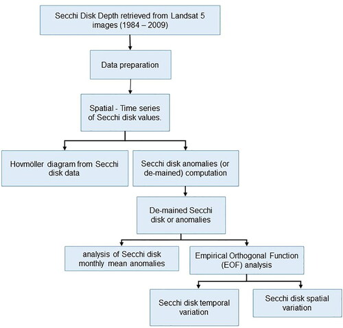
The methodological process (Figure 6) includes the following phases: data preparation to fill in missing SD values, construction of the Hovmöller diagram, anomaly analysis, and EOF analysis. In the data preparation phase, once the monthly SD data has been sorted by date, the missing data is filled in and the monthly spatial–temporal data series of the SD is constructed for each studied water body. In the second phase, the Hovmöller diagram is prepared from the monthly spatial–temporal SD series to study the spatial and temporal evolution for each lake. In the third phase, the anomalies of the SD are calculated corresponding to the variation of each monthly data with respect to the mean of the entire series for each point; for each SD value, the mean over the whole time series at that point is subtracted from the SD. Then, the anomalies of the SD are analyzed at a spatial and temporal level, calculating the multiannual mean for each month. Finally, in the fourth phase, the EOF analysis is performed from the anomalies.

Figure 6. Flow chart of the research process.

Input data

In order to evaluate the spatial and temporal variations of water quality in the PRSE, the input data are the SD values since 1984 to 2011. These values were retrieved in a previous study (Echavarría-Caballero et al. 2019) from Landsat 5 images atmospherically corrected by the USGS with software LEDAPS.

The first step of the process of obtaining the SD values was the water pixel identification method to distinguish water and non-water information. In this step, we applied the normalized difference water index (NDWI) to every available Landsat 5 image in the area under consideration. Dynamic conditions in the study area can lead to misidentified water pixels; some bodies of water may disappear completely in some seasons, and water pixels can be confused with shadows and vegetation. Therefore, we took several steps to verify the water pixels. First, we tested the fit between the result classification and the field data—that is, sampling locations in the bodies of water should fall in areas classified as water by the analysis method. Second, to certify that only open water pixels were obtained, only water bodies greater than two pixels were selected. This step was appropriate because dubious water bodies (i.e. water bodies that could be shadows or vegetation) of two or fewer pixels occurred far more frequently than dubious water bodies of three or more pixels. Third, areas belonging to river and mountain zones were also discarded to dismiss shadows, given that the water bodies under consideration are located only in flat areas. Fourth, only water pixels in the whole period (1984 to 2011) were selected—that is, pixels that are classified as water 100% of the time (light blue dashed lines in Figures 2–5).

Then, we developed a new regression equation and validated it with the SD in situ measurements and reflectance measured in the sensor bands. Finally, the SD model developed was applied to every water image (images classified so that only water information is present in the images to certify that only water pixels were used) in order to assign each pixel an SD transparency value.

Data preparation

Given that spatial–temporal series assume that there is no gap in the data, missing data were filled prior to the analysis. In the first place, to complete isolated missing values, simple interpolation methods were used since there are no significant differences from the values obtained with other more complex methods such as regression (Mukadi and González-García 2021). In the interpolation method, a missing SD value at time t was completed with the mean of the data immediately before and after it (at times t − 1 and t + 1). Missing contiguous data values were completed with the average of the previous and subsequent years. The remaining missing data were filled in with the library multivariate imputation by chained equations (MICE) in R (van Buuren and Groothuis-Oudshoorn 2011).

To validate the results of the MICE method, we used the field data of Las Madres lake (also located in the PRSE) obtained by Álvarez-Cobelas et al. (2019) since there is monthly data since 1991. Some data were randomly eliminated in order to be completed with the different MICE methods. Then, the root-mean-square error (RMSE) (Table 1) was obtained. Finally, the method with the lowest RMSE was selected and used to complete the data for the Picón de los Conejos, Campillo, Porcal, and Soto de las Cuevas pit ponds.

Table 1. Evaluated MICE library methods.

Name	Description	RMSE
cart	Classification and regression trees	0,48
midastouch	Weighted predictive mean matching	0,49
pmm	Predictive mean matching	0,55

Hovmöller diagram from SD data

Once the monthly spatial–temporal series of SD data were completed, longitude–time Hovmöller diagrams were generated to represent the temporal evolution of water transparency in each pit pond from May 1984 to December 2009. The Hovmöller diagram averages all the depth values of the SD in meters in a single column of longitude or latitude and places them on an axis. The other axis represents time.

SD anomalies (or de-meaned) computation

In order to analyze the temporal variations of the SD values, the anomalies are calculated as the subtraction of the mean of the entire time series of each point (or pixel) from each SD value (Godah et al. 2018; Hannachi et al. 2007): (1) $${\mathit{SDA}}_m\left(t\right)=\mathrm{ }{SD}_m\left(t\right)-\mathrm{ }{\mu }_m$$(1) where ${\mathit{SDA}}_m\left(t\right)$ corresponds to the SD anomaly at point m and time t (1…n); ${SD}_m\left(t\right)$ is the SD value at point m and time t; and ${\mu }_m$ is the mean of the SDs of each series, i.e. the mean of the SDs at point m. It is calculated as follows: (2) $${\mu }_m=\mathrm{ }\frac{\sum _{i=\mathrm{ }1}^n{SD}_m}{n}$$(2) where n is the number of dates to study, which is equivalent to the length of the time series.

Subsequently, we analyzed the SD anomalies. We calculated the multiannual monthly average of the anomalies at each point (${\mathit{SDA}\mu }_{m\mathrm{ }}(x)$) for the months x = 1, 2, 3, … 12, as well as the multi-year monthly average of all the points ${\mathit{SDA}\mu }_{\mathrm{ }}(x):$ (3) $${\mathit{SDA}\mu }_{m\mathrm{ }}\left(x\right)=\mathrm{ }\frac{\sum _{i=\mathrm{ }1}^n{\mathit{SDA}}_{m\mathrm{ }}\left(x\right)}{n}$$(3) (4) $${\mathit{SDA}\mu }_{\mathrm{ }}\left(x\right)=\mathrm{ }\frac{\sum _{i=\mathrm{ }1}^n{\mathit{SDA}}_{\mathrm{ }}\left(x\right)}{n}$$(4)

Empirical orthogonal function (EOF) analysis

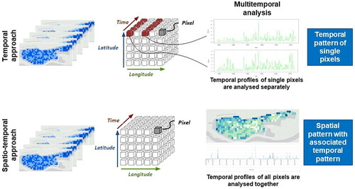
To characterize the variability of the satellite-derived SD values, an EOF was performed on the SD data set over the entire time series (1984 to 2009). EOF analysis is a statistical technique used to decompose the spatial and temporal variability of time series data sets into a few independent dominant modes. Each mode represents a certain percentage of the total variance of the data set (Figure 7) (Chen et al. 2015; Weeks et al. 2012).

Figure 7. Overview of the time series analysis of variables using the temporal and spatio-temporal approaches.

The EOF analysis was carried out with the anomalies of the SD (i.e. the variations of each value of the SD with respect to the mean of each point).

The data supporting the findings of this study are available from the corresponding author upon reasonable request.

Results and discussion

Hovmöller diagram from SD data

In the Hovmöller diagrams (Figure 8), the SD values are plotted for each east–west coordinate (on the horizontal axis) and time (on the vertical axis). The red lines located on the maps represent the minimum and maximum x coordinates, which is the area covered by the Hovmöller diagram.

Figure 8. Hovmöller diagrams for (a) Picón de los Conejos; (b) Porcal; (c) Campillo and (d) Soto de las Cuevas lakes.

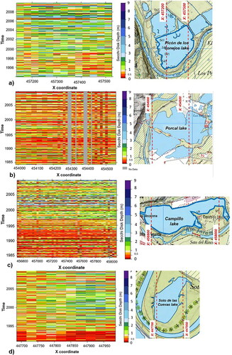
Since the Hovmöller diagrams graphically represent the mean of all the pixels in the gravel pit pond for each east–west coordinate, it is difficult to distinguish any definite spatial pattern of the SD values in such small water bodies. However, the variations of the SD values over time are clearly observed. In general terms, the transparency of the water pit ponds has improved compared to the initial study period.

In the case of Campillo lake (Figure 8c), SD values less than 0.5 meters are observed between 1985 and 1994, followed by values between 0.5 and 1 meter in 1994 to 1998, and values above 1 meter after 1998. However, between 2007 and 2009, the SE values are again below 1 meter. In the case of Picón de los Conejos lake (Figure 8a), SD values of less than 1 meter are observed not only from 1994 to 1999, but also in 2004 and from 2007 to 2009. In Porcal lake (Figure 8b) SD values of less than 1 meter are observed during the whole study period. Finally, in Soto de las Cuevas lake (Figure 8d), a period of low transparency (less than 1 meter) is observed from 1991 to 1994 and another from 2007 to 2009.

It is also visible that for the Campillo, Picón de los Conejos and Soto de las Cuevas lakes, the declaration of the regional park in 1994 had a positive impact on the water quality (Figures 8 and 9), since the SD values have increased. Nevertheless, Porcal lake shows the possible impact of anthropic activities since it is located in the area of orderly exploitation of natural resources according to the PRSE zoning.

Figure 9. Secchi disk annual means for each gravel pit pond and trophic OECD classifications.

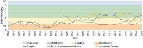
The trophic OECD classifications of lakes are as follows: hypertrophic, with annual mean SD values less than 0.75 meters; eutrophic, with SD values between 0.75 and 1.5 meters; mesotrophic, with SD values between 1.5 and 3 meters; and oligotrophic, with SD values greater than 3 meters (Giardino et al. 2001; OCDE 1982). The annual SD mean value reveals how the trophic state of pit ponds in the PRSE has changed over the years (Figure 9). Porcal lake has been classified as hypertrophic or eutrophic during the whole study period. Picón de los Conejos was mesotrophic from 1999 to 2009 except in 2001, when the trophic state was hypertrophic and eutrophic. Campillo lake has fluctuated between hypertrophic (1984–1985; 1987; 1989–1992), eutrophic (1986; 1988; 1993–1996; 1998–2000; 2005–2007) and mesotrophic (1997; 2001–2004; 2008–2009) states. Finally, Soto de las Cuevas has been classified as mesotrophic since 1996 except the period from 2006 to 2008, when the trophic state was hypertrophic and eutrophic.

According to mean SD (Figure 9), the water quality in the studied pit ponds has improved slowly since the area was declared as protected in 1994, although the ponds have not reached the oligotrophic state. There is no significant difference between the SD values of the water bodies, although Porcal has improved the least. This outcome agrees with Shevenell et al. (1999), who concluded that water quality in some pits may improve with time once exploitation ends. Given that little is known about the development of these lake ecosystems following extraction activities, further research is necessary to confirm this tendency.

These findings are relevant as they become a right tool for decision-makers to guarantee that administrative protection figures are effective to assure the sustainable management of these ecosystems. Also, this research provides the necessary data to program and plan improvement actions to comply with the Water Framework Directive (EC 2000), which requires that all water bodies must achieve good ecological status and have not been carried out in PRSE.

Monthly analysis of Secchi disk anomalies

The analysis of multi-year monthly mean anomalies of the SD values of all points (Figure 10a) allows two periods to be distinguished: a peak in autumn and winter (September–February) when the SD values are greater than the mean and a period in summer (May–August) when the SD values are lower than the mean. These results agree with Castagna et al. (2015), Naumenko (2008), Rodrigo et al. (2015), and Ziauddin et al. (2013), who concluded that when the water becomes warmer, the water transparency decreases. This trend primarily reflects the level of development of biological communities and charophyte biomass, given that the photosynthetically active radiation reaches its maximum during the warmest months.

Figure 10. (a) Monthly evolution of Secchi disk anomalies; b) box plot with the mean (blue points), minimum, maximum, median, first quartile, and third quartile.

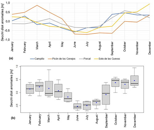
The seasonal behavior of the water bodies has little dispersion in the months of January, June, July, and August (Figure 10b). This behavior, similar in the different studied pit ponds, can be explained by the relationship between SD and temperature, given that SD is affected by two primary factors: the lake algae and suspended particulate matter (Pal & Chakraborty, 2014). These results are of great interest for the ecological management of gravel pit ponds or artificial pit ponds. Moreover, they are in agreement with other investigations such as those of lake Ladoga (Naumenko 2008) or Indian floodplain wetlands (Ziauddin et al. 2013), where equivalent results were obtained despite very different environmental conditions. The same type of environmental behavior is also observed in the case of the small shallow basin created and flooded with groundwater in a reserve area in Albufera de Valencia Natural park under the scope of a restoration program (Rodrigo et al. 2015). Global radiation and temperature increase from December to June, with maximum values in July and minimum values in December (Agencia Estatal de Meteorología de España 2017). This behavior is completely inverse to that of the SD values, where the values are lowest in July–August and highest in December–January (Figure 11).

Figure 11. Monthly evolution of Secchi disk Picón de los Conejos anomalies compared with (a) air temperature and (b) global radiation.

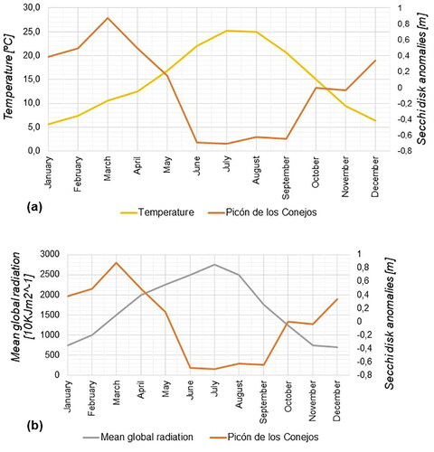
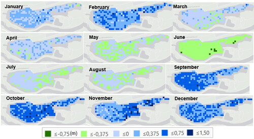
The multiannual monthly average for each pixel shows the same seasonal trends. For example, in the Campillo water pit pond, the abrupt changes occur in May and September (Figure 12). During this period, temperatures rise from 15 °C to 20 °C and solar radiation from 2,000 to 2,500 10 KJ/m². After September, temperatures fall below 20 °C and radiation decreases below 2,000 10 KJ/m² (Figure 11). No particular spatial pattern is observed.

Figure 12. Monthly spatial evolution of Secchi disk anomalies in the Campillo water pit pond.

Magnitude of change

We analyzed the magnitude or breadth of change of the SD for each pixel (Figure 13) calculated as the difference between the minimum and maximum SD values throughout the time series studied. It was observed that in Picón de los Conejos (Figure 13a) and Soto de las Cuevas (Figure 13d), pixels with a breadth of change between 5.7 and 8 meters are very frequent. In contrast, in Porcal lake (Figure 13b), there are no pixels with this amplitude, whereas the most frequent amplitudes are less than 4.6 meters. In the case of Campillo (Figure 13c), in areas whose depth is about 20 meters, the amplitude of the change in SD is less than 5.7 meters.

Figure 13. Magnitude of change of the Secchi disk for each pixel throughout the studied time series (1984–2009) for (a) Picón de los Conejos; (b) Porcal; (c) Campillo and (d) Soto de las Cuevas lakes.

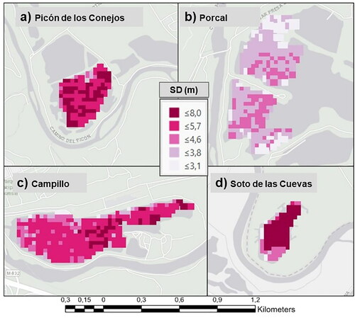
In general terms, in Porcal lake there are small fluctuations (i.e. in small ranges), while in practically the whole area of Soto de las Cuevas, Picón de los Conejos, and in specific places in Campillo there are extreme variations of more than 5.7 meters. It can be inferred that this is related to the depth of the lake, since fluctuations are smaller in deeper areas.

The behavior of Picón de los Conejos and Porcal lakes is different. These water bodies present fluctuations distributed over their entire surface, as well as very widespread spatial patterns of variability. This may be due to human intervention. Quality recovery actions are being carried out in Picón de los Conejos, while the exploitation of aggregates continues in Porcal.

Water quality variation in the studied time period

In the EOF anomalies analysis, Mode 1 explains 59.4%, 70.4%, 77.8%, and 82.6% of the spatial and temporal variability of the series for the Campillo, Picón de los Conejos, Porcal, and Soto de las Cuevas lakes, respectively.

Figure 14 shows the coefficients of each pixel for Mode 1 since this mode explains a large percentage of the variability for each water pit pond. The values that most influence the Mode 1 behavior are shown in dark blue. It can be inferred that the deeper areas have the most influence on the behavior of the time series, while the shallower areas (edges) have the least influence.

Figure 14. Mode 1 spatial variability of EOF analysis for (a) Picón de los Conejos; (b) Porcal; (c) Campillo and (d) Soto de las Cuevas lakes.

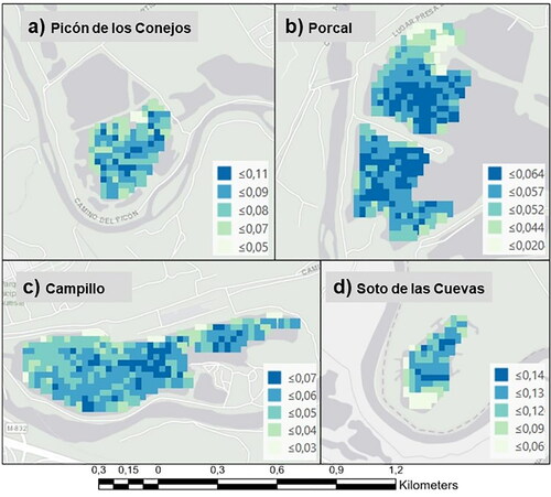
The pixels that most influence the behavior of the water pit ponds, which are in deeper areas and have a greater range of variation (Figure 13), are those that determine the general behavior of the lake. The geometry of the water pit ponds can condition their ecological evolution; as explained by Søndergaard et al. (2018), lakes with a large hypolimnion (deep area) are usually less susceptible to eutrophication than fully mixed shallow lakes. Moreover, Castagna et al. (2015) showed that lakes with a larger depth and volume generally have a lower tendency toward eutrophication.

In addition, we analyzed the temporal behavior associated with the spatial pattern (Figure 15). In this case, the bars represent the coefficient of each date for Mode 1, which explains a large percentage of the variability; the largest values represent dates that have had a greater influence on the Mode 1 behavior. In the cases of Picón de los Conejos (Figure 15a) and Porcal (Figure 15b), Mode 1 is explained—or, more fundamentally, influenced—by what has happened in recent years (larger bars), possibly reflecting human intervention in these pit ponds. On the other hand, for Campillo (Figure 15c) and Soto de las Cuevas (Figure 15d), the influence is distributed throughout the entire series with no apparent trends.

Figure 15. Mode 1 temporal variation of EOF analysis for (a) Picón de los Conejos; (b) Porcal; (c) Campillo and (d) Soto de las Cuevas lakes; the date where the year is located corresponds to May 1 for each year.

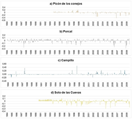
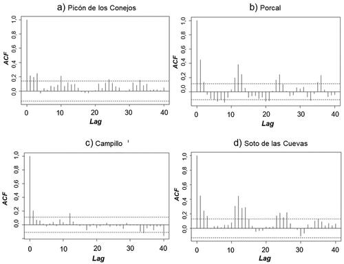
In the Porcal and Soto de las Cuevas lakes, punctual events happen throughout the series that further condition the evolution of the water pit ponds, but a seasonal temporal pattern is not observed. Therefore, the autocorrelation function (ACF) is analyzed to determine if there is any temporal pattern.

Figure 16 shows the Mode 1 autocorrelations for each studied gravel pit pond. In the case of Campillo (Figure 16c), the autocorrelations indicate a small autocorrelation around 12 and 40 lags. In Picón de los Conejos (Figure 16a), a small autocorrelation is visible in lags 10, 24, and 33. Therefore, it can be deduced that a behavior pattern is not observed in the series after 12 months. In the case of Porcal (Figure 16b) and Soto de las Cuevas (Figure 16d), the values of the SD show temporal variation with seasonality.

Figure 16. Autocorrelation function of temporal variation mode 1. (a) Picón de los Conejos; (b) Porcal; (c) Campillo and (d) Soto de las Cuevas lakes.

Practical applications

In this study, we analyzed the temporal trends and spatial distributions of water quality in water pit ponds in the PRSE by using long-term time series of water transparency retrieved by remote sensing. This technique allows the monitoring of the quality of water bodies according to the WFD (EC 2000) at low cost compared with field campaigns. As most of these water bodies are located on private lands and are therefore inaccessible, this methodology makes long-term monitoring possible. Therefore, we can also evaluate the impact of administrative and territorial planning actions, such as the 1994 declaration of a regional park.

In addition, this research has allowed us to understand whether gravel pit ponds can be compared to natural lakes in terms of seasonal behavior and the physical drivers that influence transparency, as well as to assess their ecological evolution. The environmental changes in relation to climate change can also be studied and analyzed. Therefore, this methodology is an excellent tool to support decision-making about land use practice restrictions according to the Planning and Management Plan in Protected Natural Areas of PRSE or the remedial actions to be carried out for the environmental improvement and sustainability of these ecosystems.

It is very important to have a reliable, accessible, and low-cost tool for the environmental monitoring and management of areas affected by mining activity, which remain active for many years in the metropolitan areas of large, growing cities around the world. In the case of Madrid and also in other Spanish cities, the environmental concern for this type of space is relevant (Vucic et al. 2019) due to the scarcity of aquatic ecosystems, their high environmental value, and the social importance they acquire in highly populated areas (Seelen et al. 2021).

The development of satellites with increasing spatial and temporal precision offers an enormous opportunity, which we can take advantage of by adopting the proposed methodology.

Conclusions

In this study, we examined the temporal and spatial patterns of water quality using the parameter of transparency in the Campillo, Picón de los Conejos, Porcal, and Soto de las Cuevas gravel pit ponds in the PRSE in a period of 25 years (1984–2009) using time series from Landsat 5 images.

This study highlights seasonal behavior in the water quality, with higher Secchi disk values in autumn and winter (December–February) and lower values in summer (July–August). This behavior can be explained by the relationship between SD and temperature and solar radiation.

We also used Hovmöller diagrams and the SD annual mean to show that the declaration of the Regional park in 1994 has had a positive impact on the quality of the water, since the values of the SD have increased in Campillo, Picón de los Conejos, and Soto de las Cuevas pit ponds. In contrast, the Porcal pit pond showed uniform SD values throughout the study period; this pond has been impacted by anthropic activities since it is located in the area of orderly exploitation of natural resources, according to the PRSE zoning. Furthermore, transparency (measured as SD depth) has improved compared to the initial study period in the four studied pit ponds. Also, the trophic state of the studied pit ponds has slowly improved, though it has not reached the oligotrophic state: Campillo, Picón de los Conejos, and Soto de las Cuevas have been between the eutrophic and mesotrophic states, while Porcal has been eutrophic.

According to the EOF analysis, the pixels that most influence the behavior of the pit ponds are in deeper areas and have a greater range of variation. This suggests that the geometry of the pit ponds can condition their ecological evolution. Concerning the temporal variation, in the case of Picón de los Conejos and Porcal, the variability has been more fundamentally influenced by recent developments. On the other hand, for Soto de las Cuevas and Campillo, the influence is distributed throughout the entire series without apparent trends.

This methodology elucidates the behavior of the transparency and water quality of gravel pit ponds in spatial and temporal terms. Therefore, it can be used to evaluate how previously implemented strategies have affected water quality and the ponds’ subsequent evolution toward sustainable ecosystems.

Furthermore, this methodology can be replicated with different satellite platforms, including the ESA’s new Copernicus program. Potential future applications include (i) identifying and quantifying future changes in water quality as a result of land use practice changes or other environmental changes such as climate change and (ii) comparing the obtained SD time series with levels of gravel extraction or environmental variables such as temperature or precipitation. This will allow a better understanding of the evolution of these artificial ecosystems, allowing better medium- and long-term management.

Acknowledgments

We thank to Dr. Álvarez Cobelas for providing Secchi disk field data. This research did not receive any specific grant from funding agencies in the public, commercial, or not-for-profit sectors. There are no relevant financial or non-financial competing interests to report.

Disclosure statement

No potential conflict of interest was reported by the authors.

References

- Agencia Estatal de Meteorología de España. 2017. Informe de radiación solar. https://www.bing.com/search?q=Agencia+Estatal+de+Meteorolog%C3%ADa+de+Espa%C3%B1a.+(2017).+Informe+de+radiaci%C3%B3n+solar.+Madrid&cvid=60ab20a244d74436813cfd9e0d10aef7&aqs=edge.69i57.259j0j4&pglt=2083&FORM=ANAB01&PC=LGTS.
- Álvarez-Cobelas M, Rubio A, Arauzo M, Alarcón P, Limnética VA. 1987. Morfometria y composición química de una laguna de gravera. Limnetica.Net. http://www.limnetica.net/documentos/limnetica/limnetica-3-1-p-91.pdf.
- Álvarez-Cobelas M. 1991. Optical limnology of a hypertrophic gravel‐pit lake. Int Revue Ges Hydrobiol Hydrogr. 76(2):213–223. https://doi.org/10.1002/iroh.19910760206.
- Álvarez-Cobelas M, Rojo C, Benavent-Corai J. 2019. Long-term phytoplankton dynamics in a complex temporal realm. Sci Rep. 9(1):15967. https://doi.org/10.1038/s41598-019-52333-z.
- Álvarez-Cobelas M. 2000. Estudio fisico-químico de los ambientes estancados del Parque Regional del Sureste de la Comunidad de Madrid. Centro de Investigaciones Ambientales de la Comunidad de Madrid “Fernando González Bernáldez.”
- Andrews J. 1990. Principles of restoration of gravel pits for wildlife. Br Wildlife. 2(2):80–88. https://doi.org/10.1016/0006-3207(92)91240-s.
- Beltrán-Abaunza JM, Kratzer S, Höglander H. 2017. Using MERIS data to assess the spatial and temporal variability of phytoplankton in coastal areas. Int J Remote Sens. 38(7):2004–2028. https://doi.org/10.1080/01431161.2016.1249307.
- Blanchet CC, Arzel C, Davranche A, Kahilainen KK, Secondi J, Taipale S, Lindberg H, Loehr J, Manninen-Johansen S, Sundell J, et al. 2022. Ecology and extent of freshwater browning – What we know and what should be studied next in the context of global change. Sci Total Environ. 812:152420. https://doi.org/10.1016/J.SCITOTENV.2021.152420.
- Boucher J, Weathers KC, Norouzi H, Steele B. 2018. Assessing the effectiveness of Landsat 8 chlorophyll a retrieval algorithms for regional freshwater monitoring. Ecol Appl. 28(4):1044–1054. https://doi.org/10.1002/eap.1708
- Bracher A, Xi H, Dinter T, Mangin A, Strass V, von Appen WJ, Wiegmann S. 2020. High resolution water column phytoplankton composition across the Atlantic ocean from ship-towed vertical undulating radiometry. Front Mar Sci. 7:235. https://doi.org/10.3389/fmars.2020.00235
- Castagna SED, de Luca DA, Lasagna M. 2015. Eutrophication of piedmont quarry lakes (North-Western Italy): hydrogeological factors, evaluation of trophic levels and management strategies. J Environ Assess Pol Manag. 17(04):1550036. https://doi.org/10.1142/S1464333215500362
- Chao Rodríguez Y, el Anjoumi A, Domínguez Gómez JA, Rodríguez Pérez D, Rico E. 2014. Using Landsat image time series to study a small water body in Northern Spain. Environ Monit Assess. 186(6): 3511–3522. https://doi.org/10.1007/s10661-014-3634-8
- Chen Z, Zhang SR, Coster AJ, Fang G. 2015. EOF analysis and modeling of GPS TEC climatology over North America. J Geophys Res Space Phys. 120(4):3118–3129. https://doi.org/10.1002/2014JA020837
- Chu HJ, Kong SJ, Chang CH. 2018. Spatio-temporal water quality mapping from satellite images using geographically and temporally weighted regression. Int J Appl Earth Obs Geoinf. 65:1–11. https://doi.org/10.1016/J.JAG.2017.10.001
- Comunidad de Madrid. 2020. Plan de Actuación sobre Humedales Catalogados de la Comunidad de Madrid. Madrid – Bing. https://www.bing.com/search?q=Plan+de+Actuaci%C3%B3n+sobre+Humedales+Catalogados+de+la+Comunidad+de+Madrid.+Madrid&qs=n&form=QBRE&msbsrank=0_0__0&sp=-1&pq=plan+de+actuaci%C3%B3n+sobre+humedales+catalogados +de+la+comunidad+de+madrid.+madrid&sc=0-79&sk=&cvid=1790048BAEA54D62B99D5E207A1741E4.
- Cressie N, Wikle C. 2015. Statistics for spatio-temporal data. https://books.google.com/books?hl=es&lr=&id=4L_dCgAAQBAJ&oi=fnd&pg=PP1&ots=idWU3BNn0-&sig=itYykh_C0wyLAKxBD5PUlXtyuR8.
- Delasalles E, Ziat A, Denoyer L, Gallinari P. 2019. Spatio-temporal neural networks for space-time data modeling and relation discovery. Knowl Inf Syst. 61(3):1241–1267. https://doi.org/10.1007/S10115-018-1291-X/TABLES/5
- Devlin MJ, Petus C, da Silva E, Tracey D, Wolff NH, Waterhouse J, Brodie J. 2015. Water quality and river plume monitoring in the Great Barrier Reef: an overview of methods based on ocean colour satellite data. Remote Sens. 7(10):12909–12941. https://doi.org/10.3390/RS71012909
- Díaz JMC, Araujo JM. 2017. Historic urbanization process in Spain (1746–2013): from the fall of the American empire to the real estate bubble. J Urban Hist. 43(1):33–52. https://doi.org/10.1177/0096144215583481
- Domínguez Gómez JA, Chuvieco Salinero E, Sastre Merlín A. 2009. Monitoring transparency in inland water bodies using multispectral images. Int J Remote Sens. 30(6):1567–1586. https://doi.org/10.1080/01431160802513811
- Domínguez Gómez JA, Peña R. 1999. Trophic state assessment in two gravel pits (El Campillo & El Porcal) using airborne imagery. Limnetica.16(1).
- EC. 2000. Directive 2000/60/EC of the European Parliament and of the Council of 23 October 2000 establishing a framework for Community action in the field of water policy. Off J Eur Parliam. :1–73.
- Echavarría-Caballero C, Domínguez-Gómez JA, González-García C, García-García MJ. 2019. Assessment of Landsat 5 images atmospherically corrected with LEDAPS in water quality time series. Can J Remote Sens. 45(5):691–706. https://doi.org/10.1080/07038992.2019.1674136
- el Serafy GYH, Schaeffer BA, Neely MB, Spinosa A, Odermatt D, Weathers KC, Baracchini T, Bouffard D, Carvalho L, Conmy RN, et al. 2021. Integrating inland and coastal water quality data for actionable knowledge. Remote Sens. 13(15):2899. https://doi.org/10.3390/RS13152899
- Giardino C, Pepe M, Brivio PA, Ghezzi P, Zilioli E. 2001. Detecting chlorophyll, Secchi disk depth and surface temperature in a sub-alpine lake using Landsat imagery. Sci Total Environ. 268(1–3):19–29. https://doi.org/10.1016/S0048-9697(00)00692-6
- Godah W, Szelachowska M, Krynski J. 2018. Application of the PCA/EOF method for the analysis and modelling of temporal variations of geoid heights over Poland. Acta Geod Geophys. 53(1):93–105. https://doi.org/10.1007/s40328-017-0206-8
- Hannachi A, Jolliffe IT, Stephenson DB. 2007. Empirical orthogonal functions and related techniques in atmospheric science: a review. Int J Climatol. 27(9):1119–1152. https://doi.org/10.1002/joc.1499
- Hestir EL, Brando VE, Bresciani M, Giardino C, Matta E, Villa P, Dekker AG. 2015. Measuring freshwater aquatic ecosystems: the need for a hyperspectral global mapping satellite mission. Remote Sens Environ. 167:181–195. https://doi.org/10.1016/j.rse.2015.05.023
- Hicks BJ, Stichbury GA, Brabyn LK, Allan MG, Ashraf S. 2013. Hindcasting water clarity from Landsat satellite images of unmonitored shallow lakes in the Waikato region. New Zealand Environ Monit Assess. 185(9):7245–7261. https://doi.org/10.1007/s10661-013-3098-2
- Kim SE, Seo IW, Choi SY. 2017. Assessment of water quality variation of a monitoring network using exploratory factor analysis and empirical orthogonal function. Environ Modell Software. 94:21–35. https://doi.org/10.1016/j.envsoft.2017.03.035
- Kim SH, Yang CS, Ouchi K. 2015. Spatio-temporal patterns of Secchi depth in the waters around the Korean Peninsula using MODIS data. Estuarine Coastal Shelf Sci. 164:172–182. https://doi.org/10.1016/j.ecss.2015.07.003
- Li X, Yang C, Zhang H, Wang P, Tang J, Tian Y, Zhang Q. 2021. Identification of abandoned Jujube fields using multi-temporal high-resolution imagery and machine learning. Remote Sens. 13(4):801. https://doi.org/10.3390/rs13040801
- Liew SC, Chia AS, Kwoh LK. 2010. Spatio-temporal variability of precipitation in Southeast Asia analyzed using the empirical orthogonal function (EOF) technique. International Geoscience and Remote Sensing Symposium (IGARSS), 4701–4704.
- Liu D, Yu SJ, Xiao QT, Qi TC, Duan HT. 2021. Satellite estimation of dissolved organic carbon in eutrophic Lake Taihu, China. REMOTE Sens Environ. 264:112572. https://doi.org/10.1016/j.rse.2021.112572
- Lobo F, de L, Nagel GW, Maciel DA, de Carvalho LAS, Martins VS, Barbosa CCF, de Moraes Novo EML. 2021. Algaemap: algae bloom monitoring application for inland waters in Latin America. Remote Sens. 13(15):2874. https://doi.org/10.3390/RS13152874
- López-Andreu FJ, Erena M, Dominguez-Gómez JA, López-Morales JA. 2021. Sentinel-2 images and machine learning as tool for monitoring of the common agricultural policy: Calasparra rice as a case study. Agronomy. 11(4):621. https://doi.org/10.3390/AGRONOMY11040621
- Maeda EE, Lisboa F, Kaikkonen L, Kallio K, Koponen S, Brotas V, Kuikka S. 2019. Temporal patterns of phytoplankton phenology across high latitude lakes unveiled by long-term time series of satellite data. Remote Sens Environ. 221:609–620. https://doi.org/10.1016/j.rse.2018.12.006
- Mollema P, Antonellini M, Gabbianelli G, Laghi M, Marconi V, Minchio A. 2012. Climate and water budget change of a Mediterranean coastal watershed, Ravenna, Italy. Environ Earth Sci. 65(1):257–276. https://doi.org/10.1007/s12665-011-1088-7
- Mollema P, Antonellini M. 2016. Water and (bio)chemical cycling in gravel pit lakes: a review and outlook. Earth-Sci Rev. 159:247–270. https://doi.org/10.1016/j.earscirev.2016.05.006
- Mollema P, Stuyfzand P, Juhász-Holterman MHA, van Diepenbeek PMJA, Antonellini M. 2015. Metal accumulation in an artificially recharged gravel pit lake used for drinking water supply. J Geochem Explor. 150:35–51. https://doi.org/10.1016/j.gexplo.2014.12.004
- Moreno N, García-Avilés J. 1997. Valoración ambiental y caracterización de los ecosistemas acuáticos leníticos del Parque Regional en torno a los ejes de los cursos bajos de los ríos. https://www.researchgate.net/profile/Javier-Garcia-Aviles/publication/297387060_Valoracion_ambiental_y_caracterizacion_de_los_ecosistemas_acuaticos_leniticos_del_Parque_Regional_en_torno_a_los_ejes_de_los_cursos_bajos_de_los_rios_Manzanares_y_Jarama/links/56deb0c408ae46f1e9a0e3eb/Valoracion-ambiental-y-caracterizacion-de-los-ecosistemas-acuaticos-leniticos-del-Parque-Regional-en-torno-a-los-ejes-de-los-cursos-bajos-de-los-rios-Manzanares-y-Jarama.pdf.
- Mostaza-Colado D, Carreño-Conde F, Rasines-Ladero R, Iepure S. 2018. Hydrogeochemical characterization of a shallow alluvial aquifer: 1 baseline for groundwater quality assessment and resource management. Sci Total Environ. 639:1110–1125. https://doi.org/10.1016/j.scitotenv.2018.05.236
- Mukadi PM, González-García C. 2021. Time series analysis of climatic variables in peninsular spain. trends and forecasting models for data between 20th and 21st centuries. Climate 2021. 9(7):119. https://doi.org/10.3390/CLI9070119
- Nas B, Ekercin S, Karabörk H, Berktay A, Mulla DJ. 2010. An application of landsat-5TM image data for water quality mapping in Lake Beysehir, Turkey. Water Air Soil Pollut. 212(1–4):183–197. https://doi.org/10.1007/s11270-010-0331-2
- Naumenko MA. 2008. Seasonality and trends in the Secchi disk transparency of Lake Ladoga. Hydrobiologia. 599(1):59–65. https://doi.org/10.1007/s10750-007-9198-7
- OCDE. 1982. OECD: eutrophication of waters. monitoring, assessment and control. 154pp Paris: organisation for economic co-operation and development 1982. Int Revue Der Gesamten Hydrobiol Und Hydrograph. 69(2):200.
- Pal S, Chakraborty K. 2014. Importance of some physical and chemical characteristics of water bodies in relation to the incidence of zooplanktons: a review. Indian Journal of Social and Natural Sciences. 3:102–116.
- Paltsev A, Creed IF. 2021. Are northern lakes in relatively intact temperate forests showing signs of increasing phytoplankton biomass? Ecosystems. https://doi.org/10.1007/s10021-021-00684-y
- Peckenham JM, Thornton T, Whalen B. 2009. Sand and gravel mining: effects on ground water resources in Hancock county, Maine, USA. Environ Geol. 56(6):1103–1114.
- Persson A. 2017. The story of the Hovmöller diagram: an (almost) eyewitness account. Bull Am Meteorol Soc. 98(5):949–957.
- Rodrigo M, Rojo C, Segura M, Alonso-Guillén J, Martín M, Vera P. 2015. The role of charophytes in a Mediterranean pond created for restoration purposes. Elsevier. https://www.sciencedirect.com/science/article/pii/S0304377014000692.
- Seelen LMS, Teurlincx S, Bruinsma J, Huijsmans TMF, van Donk E, Lürling M, de Senerpont Domis LN. 2021. The value of novel ecosystems: disclosing the ecological quality of quarry lakes. Sci Total Environ. 769:144294.
- Seers BM, Shears NT. 2015. Spatio-temporal patterns in coastal turbidity – long-term trends and drivers of variation across an estuarine-open coast gradient. Estuarine Coastal Shelf Sci. 154:137–151. https://doi.org/10.1016/j.ecss.2014.12.018
- Shevenell L, Connors KA, Henry CD. 1999. Controls on pit lake water quality at sixteen open-pit mines in Nevada. Appl Geochem. 14(5):669–687. https://doi.org/10.1016/S0883-2927(98)00091-2
- Søndergaard M, Lauridsen TL, Johansson LS, Jeppesen E. 2018. Gravel pit lakes in Denmark: chemical and biological state. Sci Total Environ. 612:9–17. https://doi.org/10.1016/j.scitotenv.2017.08.163
- U.S. Geological Survey. 2015. Mineral commodity summaries 2015 mineral commodity summaries 2015. US Geological Survey. http://www.usgs.gov/pubprod%0Ahttps://minerals.usgs.gov/minerals/pubs/commodity/phosphate_rock/mcs-2015-phosp.pdf.
- van Buuren S, Groothuis-Oudshoorn K. 2011. mice: multivariate imputation by chained equations in R. J Stat Soft. 45(3):1–67. https://doi.org/10.18637/jss.v045.i03
- Vucic JM, Cohen RS, Gray DK, Murdoch AD, Shuvo A, Sharma S. 2019. Young gravel-pit lakes along Canada’s Dempster highway: how do they compare with natural lakes? Arctic Antarctic Alpine Res. 51(1):25–39. https://doi.org/10.1080/15230430.2019.1565854
- Wang R, Yan X, Niu Z, Chen W. 2021. Long-term changes in inland water surface temperature across china based on remote sensing data. J Hydrometeorol. 22(2):523–532. https://doi.org/10.1175/JHM-D-20-0104.1
- Weeks S, Werdell PJ, Schaffelke B, Canto M, Lee Z, Wilding JG, Feldman GC. 2012. Satellite-derived photic depth on the Great Barrier Reef: spatio-temporal patterns of water clarity. Remote Sensing. 4(12):3781–3795. https://doi.org/10.3390/rs4123781
- Yoder JA, Schollaert SE, O'Reilly JE. 2002. Climatological phytoplankton chlorophyll and sea surface temperature patterns in continental shelf and slope waters off the northeast U.S. coast. Limnol Oceanogr. 47(3):672–682. https://doi.org/10.4319/lo.2002.47.3.0672
- Ziauddin G, Chakraborty SK, Jaiswar AK, Bhaumik U. 2013. Productivity study in relation to temperature and transparency in the euphotic zone of selected tropical freshwater floodplain wetlands of West Bengal. N Save Nature to Survive (Vol. 7, Issue 4). https://www.researchgate.net/publication/280832042.