High-spatial-resolution remote sensing image segmentation using adaptive watershed-driven joint MDEDNet

Abstract

When segmenting high-spatial-resolution remote sensing images using convolution neural networks, it is difficult to balance the number of segmented regions against the contour accuracy. This article proposes a segmentation method that combines the minimum area adaptive watershed transform based on morphological reconstruction with the modified deep edge detection network (MDEDNet). First, the minimum area adaptive watershed algorithm is adopted to reconstruct the gradient features of the image and perform watershed segmentation, giving the initial segmentation results. A ground object contour optimization method and MDEDNet are then used to further improve the accuracy of the segmentation, resulting in the final segmented image. Experiments on image sets of varying complexity indicate that the algorithm proposed in this article can achieve accurate image segmentation with good segmentation results and fast operation efficiency.

Keywords:

• Deep convolution neural network model
• morphological reconstruction
• minimum area
• adaptive watershed transform
• MDEDNet

1. Introduction

With the rapid development of Earth observation technology, high-resolution remote sensing images have been widely used for urban management, crop inversion and classification and disaster monitoring. Compared with medium- and low-resolution remote sensing images, high-resolution imagery provides abundant information on texture structure, clearer information on the contours and shape of ground objects, as well as identifying more complex and diverse relationships between ground objects. Therefore, there are many new challenges in the interpretation, information extraction and analysis of high-resolution remote sensing images.

High-resolution image segmentation is the basis of interpreting and extracting information from high-resolution remote sensing images. This is the key step in realizing data mining and ‘informationization’, and is thus a research hotspot in the process of image processing. At present, image segmentation methods can be divided into low-, mid- and high-level semantic methods. Low-level semantic segmentation is based on color, texture and shape information of image pixels, and uses threshold segmentation and boundary segmentation. The threshold segmentation method only considers the spectral features of the image, but it does not fully consider other features such as the spatial relationship between the pixels (Zhang et al. 2018). Thus, the threshold segmentation method is easy to be implemented, and the execution speed is faster than the clustering algorithm-based segmentation method. When the grey-level value of the target area differs greatly from other features, this method can effectively perform segmentation, especially in colour images. Nevertheless, when the grey-level difference is minimal or a large overlap of the grey-level range occurs in the image, the segmentation region is likely to be discontinuous with obvious noise. The boundary segmentation detects edges and creates segment polygons to achieve high-spatial-resolution remote sensing image segmentation based on the discontinuities of pixels in different regions. If the difference between the regions is obvious, the segmentation results are better. Conversely, if the boundary between the regions is blurred or the boundaries are numerous and the noise robustness is poor, then the image texture region cannot be segmented well, and obtaining an ideal closed boundary is difficult .Therefore, this kind of method can realize fast image segmentation, but may ignore information about the spatial structure of the image and is sensitive to noise (Drever et al. 2007; Huo et al. 2017; Yamini and Sabitha 2017). Low-level semantic segmentation is not often used for the segmentation of high-resolution remote sensing images.

Mid-level semantic segmentation, such as the super-pixel segmentation first proposed by Ren, refers to local subregions composed of local pixels with the same properties in an image (Ren and Malik 2003). These subregions are typically identified by clustering methods and graph theory methods. The clustering methods represents pixels in the image space with their corresponding feature space points, and forms a separate class by clustering the points in the feature space (Sun et al. 2008). The clustering methods have high computational efficiency, and most can control the number of initial super-pixels. However, when the clustering method is used for high-spatial-resolution remote sensing image segmentation, it ignores the rich spatial information other than the grey-level features of the high-spatial-resolution remote sensing image segmentation, making it easy to obtain inaccurate segmentation results. The graph theory-based high-spatial-resolution remote sensing image segmentation method transforms the segmentation problem into a high-spatial-resolution remote sensing image segmentation optimisation problem. The graph theory methods do not depend on the edge and texture features of the image, so they produce a better segmentation effect with images containing high noise intensity, uneven gray scale, low contrast or fuzzy target boundaries. Therefore, this method is computationally complex, and the segmentation results depend on the initial contour selection of the ground object edge, which leads to poor segmentation accuracy of ground object boundaries (Achanta et al. 2012; Achanta and Susstrunk 2017; Fang et al. 2018; Rémi et al. 2018). mid-level semantic segmentation is only suitable for the pre-segmentation of high-resolution remote sensing images (Rother et al. 2004; Farabet et al. 2013; Bai and Chen 2016; Nakamura and Byung-Woo 2016; Shen et al. 2016; Yu et al. 2016; Mahaman et al. 2017; Awaisu et al. 2019).

In recent years, the rapid development of deep learning has attracted much attention. Deep learning plays a key role in the fields of image segmentation (Abdollahi et al. 2021), image recognition (Wu and Chen 2015), object detection (Zhao et al. 2015), speech recognition (Deng et al. 2013) and image classification (Biswajeet et al. 2020). It, therefore, provides important decision support in a variety of situations. High-level semantic segmentation is a deep learning-based high-spatial-resolution remote sensing image segmentation method. With the continuous development of high-resolution remote sensing image segmentation, the impact of the phenomenon of ‘same object with different spectra’ and ‘different object with same spectra’ is increasing, and the accuracy of traditional high-spatial- resolution remote sensing image segmentation methods is poor. As a result, the deep learning-based high-spatial-resolution remote sensing image segmentation method is gradually developing. Long et al. (2014) first proposed an end-to-end full convolution network (FCN), which adopts the idea of fusing low- and high-level semantic features, and uses a transposed convolution layer (instead of a full connection layer) as the decoder for converting from image pixels to pixel categories. Compared with classical convolution neural networks (CNNs), FCN effectively improves the accuracy of image semantic segmentation and creates a codec network structure that lays the foundation for various image semantic segmentation networks. However, this segmentation method will lead to image objects with poor edges. Wang et al. (2019) proposed a C model that has a detailed decoding module whereby the feature image is integrated with the features identified by the coding module, thus reducing the boundary blurring problem of some ground objects. Deng et al. (2018) developed a weighted cross-entropy loss function method, which reduces the problems faced by boundary detection models. The main problem with the above mentioned methods is rooted in the network framework of deep learning, in which the pooling layer leads to blurred edge output and the convolution layer interferes with adjacent ground object pixels. These issues make it impossible to generate accurate ground object segmentation images.

In summary, it is difficult to balance the number of segmented regions and the contour accuracy in deep convolution neural network models for high-resolution remote sensing image segmentation. Additionally, many existing methods cannot simultaneously satisfy the requirements for fast and effective segmentation. This article proposes a method that achieves fast pre-segmentation of images using an adaptive watershed based on morphological reconstruction. This not only solves the problem of over-segmentation and parameter optimization in the morphological reconstruction algorithm, but also addresses the problem of balancing the number of segmented regions with the contour accuracy. The modified deep edge detection network (MDEDNet) is used to expand the architecture of traditional networks to extract detailed features, with a skip connection used to improve the gradient flow across a large number of layers and different activation images at different levels combined to output accurate and clear edges of ground objects. The motivation behind using MDEDNet is that multiscale structuring elements are employed to reconstruct a gradient image, i.e. small structuring elements are adopted by pixels of large gradient magnitude while large structuring elements are adopted by pixels of small gradient magnitude. These two properties help segmentation algorithms to achieve better hierarchical segmentation. As a result, the proposed method achieves the accurate segmentation of high-resolution remote sensing images.

The remainder of this article is organised as follows. Section 2 describes the proposed pre-segmentation method MDEDNet, a ground object contour optimisation method. In Section 3, the proposed method is used for seeded image segmentation, to demonstrate its superiority. Finally, in Section 5, we discuss our work concerning possible future directions. We have written the alteration into page 3, paragraph 2.

2. Methods

The algorithm proposed in this article is mainly composed of two parts. First, we employ the minimum area adaptive watershed transform of morphological reconstruction (MR-MAA-WS) to realize pre-segmentation. Then, a ground object contour optimization method and MDEDNet are used to improve the accuracy of the pre-segmentation results, giving the final segmented image. The overall process is shown in Figure 1.

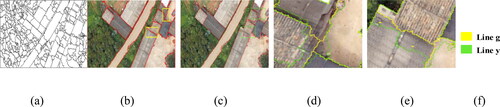
Figure 1. Proposed image segmentation framework. (a) Original image; (b) Gradient image using Sobel operator; (c) Segmentation result of watershed transform based on morphological reconstruction (MR-WS); (d) Adaptive morphological reconstruction (AMR) of (b); (e) Regional minimum image; (f) Segmentation result of MR-MAA-WS; (g) Contour prediction based on MDEDNet; (h) Final segmentation result.

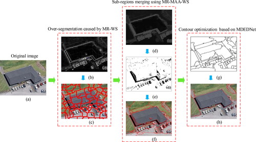
The proposed method has the following advantages:

1. MR-MAA-WS provides better pre-segmentation results for high-resolution remote sensing images. This is because the parameters of the initial structural elements in the reconstructed image are removed. In addition, over-segmentation from the watershed algorithm is significantly reduced.

2. Improved edge optimization is achieved through MDEDNet. Combining MR-MAA-WS with MDEDNet allows the advantages of both approaches to be harnessed, i.e. the correct segmentation area is obtained, and more accurate contour positioning is achieved. The pre-segmentation results of the watershed algorithm are modified by the MDEDNet contour prediction results, leading to obviously improved segmentation accuracy.

2.1. Minimum area adaptive watershed transform based on morphological reconstruction

2.1.1. Adaptive multiscale morphological reconstruction

High-resolution remote sensing images contain amplitude noise and scale noise. Although several multiscale adaptive morphological algorithms reduce the influence of noise (Fan et al. 2008; Xu et al. 2008; Li et al. 2010; Zhang et al. 2018), they output the average results of morphological operations at all scales, resulting in contour offset and errors. Opening and closing operations can greatly reduce the impact of ground object contour segmentation errors on the watershed segmentation algorithm, as shown in Eqs. (1)(1) $$O_B^{\left(\mathrm{rec}\right)}\left(g,f_{\delta }\right)=D_B^{\left(\mathrm{rec}\right)}\left[\left(\left(g\right),\epsilon b_i\right)\right]\mathrm{ },$$(1) and (2)(2) $$C_B^{\left(\mathrm{rec}\right)}\left(g,f_{\epsilon }\right)=E_B^{\left(\mathrm{rec}\right)}\left[\left(\left(g\right),\delta b_i\right)\right]\mathrm{ },$$(2) . However, a single-scale structural element will mistakenly be selected as the seed point, whereby both large and small structural elements will be poorly reconstructed, and the medium structural elements must achieve a rough balance through accurate contours. Thus, it is necessary to select appropriate seed points. This article proposes an adaptive morphological reconstruction (AMR) algorithm that adaptively completes small structural elements with large gradient pixels and large structural elements with small gradient pixels on the basis of the morphological reconstruction of multiscale structural elements. First, the algorithm filters useless gradient information adaptively, while retaining meaningful seed points. Second, multiscale structural elements with the characteristics of monotonic increments and convergence are used to achieve the adaptive segmentation of gradient images. (1) $$O_B^{\left(\mathrm{rec}\right)}\left(g,f_{\delta }\right)=D_B^{\left(\mathrm{rec}\right)}\left[\left(\left(g\right),\epsilon b_i\right)\right]\mathrm{ },$$(1) (2) $$C_B^{\left(\mathrm{rec}\right)}\left(g,f_{\epsilon }\right)=E_B^{\left(\mathrm{rec}\right)}\left[\left(\left(g\right),\delta b_i\right)\right]\mathrm{ },$$(2) where $O_B^{\left(\mathrm{rec}\right)}\left(g,f_{\delta }\right)$ is an opening operation, $C_B^{\left(\mathrm{rec}\right)}\left(g,f_{\epsilon }\right)$ is a closing operation, and $D_B^{\left(\mathrm{rec}\right)},$ $E_B^{\left(\mathrm{rec}\right)}$ are the results of morphological dilation and corrosion. (3) $$\phi \left(g,s,m\right)=\underset{s\le i\le m}{\bigvee }\left\{C_B^{\left(\mathit{rec}\right)}{\left(f_{\epsilon }\right)}_{b_i}\right\}\mathrm{ },$$(3) where $\phi$ is an adaptive morphological reconstruction operator, which increases with the scale of structural elements and satisfies the conditions $f_{\epsilon }\left(x,y\right)=\left(\epsilon b_i\left(g\right)\right)$ and $f\le g.$ In Eq. (3)(3) $$\phi \left(g,s,m\right)=\underset{s\le i\le m}{\bigvee }\left\{C_B^{\left(\mathit{rec}\right)}{\left(f_{\epsilon }\right)}_{b_i}\right\}\mathrm{ },$$(3) , $\mathrm{Ⅴ}$ represents the maximum operation of morphological reconstruction, i.e. the maximum value of image pixels. Let the structural element of morphological reconstruction be $b_s,\mathrm{ }{b}_i,\mathrm{ }{b}_{i+1}\mathrm{ },...b_m$ , where i is the scale parameter of the structural element, $1\le s\le i\le m$ , $s,\mathrm{ }i,\mathrm{ }m\in n^{+}.$ A large value of s will lead to the merging of small areas, and the accuracy of the object contours will be reduced.

A pixel-by-pixel maximum operation is applied to $C_B^{\left(\mathrm{rec}\right)}{\left(f_{\epsilon }\right)}_{b_i},$ but not to $O_B^{\left(\mathrm{rec}\right)}{(g,f}_{\delta }).$ Because , $\underset{m\to \mathrm{\infty }}{\lim }{C}_B^{\left(\mathrm{rec}\right)}{\left(f_{\epsilon }\right)}_{b_i}=\max \left(g\right)$ , $\underset{m\to \mathrm{\infty }}{\lim }\underset{s\le i\le m}{\bigvee }\left\{C_B^{\left(\mathrm{rec}\right)}{\left(f_{\epsilon }\right)}_{b_i}\right\}=\max \left(g\right)$ and $\phi \left(g,\mathrm{ }s,\mathrm{ }m\right)$ is unable to obtain convergent gradient images.

The algorithm proposed in this article contains two parameters, s and m. The computational efficiency of adaptive morphological reconstruction is affected by m. A smaller value of m corresponds to lower computational complexity. When $\left(g,\mathrm{ }s,\mathrm{ }m\right)\ge C_B^{\left(\mathrm{rec}\right)}{\left(f_{\epsilon }\right)}_{b_i}$, the reconstructed gradient image and the corresponding segmentation result remain unchanged, but the resulting value of m is usually large. Because the purpose of this article is to improve the seed segmentation algorithm by using adaptive morphological reconstruction, the convergence condition $\phi \left(g,\mathrm{ }s,\mathrm{ }m\right)\ge C_B^{\left(\mathrm{rec}\right)}{\left(f_{\epsilon }\right)}_{b_i}$ is replaced by checking the difference between $\phi \left(g,\mathrm{ }s,\mathrm{ }m\right)$ and $\phi \left(g,\mathrm{ }s,\mathrm{ }m-1\right).$ The objective function of convergence is defined as follows: (4) $$J\left(g,s\right)=\max \left|\phi \left(g,\mathrm{ }s,\mathrm{ }m\right)-\phi \left(g,\mathrm{ }s,\mathrm{ }m-1\right)\right|\mathrm{ },$$(4) where $\ge 2$ , $m\in n^{+}.$ Obviously, when $j\le \eta ,$ where η is the (constant) minimum threshold error, the segmentation result will remain unchanged. However, m is a variable of $\left(g,\mathrm{ }s,\mathrm{ }m\right)$ , so only the parameter s needs to be adjusted by the adaptive morphological reconstruction parameters. The three parameters s, m and η are used because the iteration can be stopped according to m or η. The computational complexity of adaptive morphological reconstruction depends on the value of m or η. Larger values of m correspond to smaller values of η. As m increases, the execution time of the algorithm becomes longer. Therefore, two convergence conditions for m and η are used to accelerate the convergence of the algorithm.

2.1.2. MR-MAA-WS algorithm

Gradient images are sensitive to noise, so the watershed transform (Zhang and Zhang 2017) often produces an over-segmentation effect. (Lei et al. 2019) Additionally, gradient images usually contain a large number of regional minimums, which again leads to over-segmentation. Therefore, we introduce an adaptive morphological reconstruction algorithm based on the watershed transform (AMR-WS). This algorithm has the properties of monotonicity and convergence, and adaptively obtains the segmentation threshold, thus, effectively reducing the problem of over-segmentation. However, a new problem is introduced: all parameters of the proposed algorithm need to be properly adjusted according to the remote sensing image features. Although the adjustment of parameters can be guided by a series of rules, the optimal segmentation parameters are still obtained by empirical values (Lei et al. 2019), which is not ideal for the realization of automatic image segmentation.

To further improve the algorithm by overcoming the problems of the use of image geometric information and the selection of initial structural elements, the method of region merging is adopted. This allows the number of small regions to be reduced while preserving the boundary accuracy. Removing the minimum connected component of the adaptive multiscale morphological reconstruction results allows the gradient image to be further optimized. This reduces the occurrence of over-segmentation, and is equivalent to region merging.

When s is sufficiently large (i.e. the parameter value of the initial structural element is equal to the maximum value m), AMR reduces to MR. Thus, the parameter s can be removed and a simpler representation appears. (5) $$\phi \left(g,m\right)={\bigvee }_{1\le i\le m}\left\{R_g^{\varphi }{\left(f_{\epsilon }\right)}_{b_i}\right\},$$(5)

According to Eq. (5)(5) $$\phi \left(g,m\right)={\bigvee }_{1\le i\le m}\left\{R_g^{\varphi }{\left(f_{\epsilon }\right)}_{b_i}\right\},$$(5) , a segmentation result with higher boundary accuracy is obtained, but the segmentation result contains more small regions, as shown in Figure 2.

Figure 2. Improved segmentation result. (a) Original image; (b) Gradient image optimization using AMR-WS (s = 1, η = 0.001); (c) Image segmentation result based on (b); (d) Regional minimum image; (e) Segmentation result of MR-MAA-WS (k = 1).

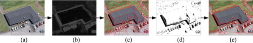
As can be seen in Figure 2(d), the minimum image of the region contains many small connection components. To address this problem, we propose the following theorem as a means of obtaining Figure 2(e).

Theorem 1.

Let g be the gradient image, I be the local minimum image of g and W be the final segmentation result using the watershed transformation. I =(I1, I2, ···, In), where Ij represents the connected components in the jth region of I, $1\le j\le n$. Similarly, $=w_1\cup w_2\cup ,...,w_n$ , represents the jth segmented region in image W. According to $I_j\subseteq W_j$, we have that (6) $${\sum }_{p\in w_j}\theta \left(x_p\right)\ge {\sum }_{q\in I_j}\theta \left(x_q\right),$$(6) (7) $$\theta \left(x_i\right)=\{\begin{array}{c}1 x_i\in W_j\mathit{\text{ or }}{I}_j\\ 0 \mathit{otherwise}\end{array}\mathrm{ },,$$(7)

where $w_{j1}\cup w_{j2}=\mathrm{\varnothing },$ $1\le j_{1\mathrm{ }},\mathrm{ }{j}_2\le n\mathrm{ },\mathrm{ }{j}_1\ne j_2,$ $x_p$ is the pth pixel of W in image I and $x_q$ is the qth pixel of W in image I. It can be seen from Eqs. (6)(6) $${\sum }_{p\in w_j}\theta \left(x_p\right)\ge {\sum }_{q\in I_j}\theta \left(x_q\right),$$(6) and (7)(7) $$\theta \left(x_i\right)=\{\begin{array}{c}1 x_i\in W_j\mathit{\text{ or }}{I}_j\\ 0 \mathit{otherwise}\end{array}\mathrm{ },,$$(7) that it is possible to merge smaller segmented regions by deleting smaller connection components in image I. The regional minimum image is a binary image, for which geometric information is more useful than gray information. Based on the binary morphological operation and Theorem 1, binary morphological reconstruction can be used to delete smaller connection components, so as to realize region merging in the segmentation results. The following formula is used to delete connected components: (8) $$I^r=R_I^{\epsilon }\left(\epsilon \left(I\right)b_k\right)\mathrm{ },$$(8) where k represents the parameter of the structural elements. According to Eq. (8)(8) $$I^r=R_I^{\epsilon }\left(\epsilon \left(I\right)b_k\right)\mathrm{ },$$(8) , it is easy to merge small areas in image W by setting the value of k. In addition, larger values of k mean that more areas are merged. In AMR-WS, the parameters s, m and η are needed for the calculation, and two stop conditions are adopted to speed up the execution of the algorithm. In MR-MAA-WS, the parameter s is no longer necessary, but the new parameter k is introduced. However, the improved boundary accuracy means that MR-MAA-WS is superior to AMR-WS.

The detailed process of MR-MAA-WS is described in Algorithm 1.

Table

Algorithm 1: Minimum area adaptive watershed transform based on morphological reconstruction (MR-MAA-WS)
Step 1: Input an image $F\left(x,y\right)$ and generate a gradient image $g(x,y)=G(F)\mathrm{ };$
Step 2: Initialize: set values for k, m (the scale of the minimal and maximal structural elements) and η, and set convergence conditions for both m and η ;
Step 3: Compute $C_B^{\left(\mathrm{rec}\right)}{\left(f_{\epsilon }\right)}_{b_i},$ where $f_{\epsilon }\left(x,y\right)=\left(\epsilon b_i\left(g\right)\right)$ , bi is a structural element, $1\le i\le m;$
Step 4: Update $\phi \left(g,\mathrm{ }m\right)$ and $J\left(g,\mathrm{ }m\right)$ ; 1) If $i=1,$ then compute $\phi \left(g,\mathrm{ }i\right){=C}_B^{\left(\mathrm{rec}\right)}{\left(f\right)}_{b_i}$ and $J=\phi \left(g,\mathrm{ }i\right){=C}_B^{\left(\mathit{rec}\right)}{\left(f\right)}_{b_i}$ ; 2) Else, compute $\phi \left(g,\mathrm{ }i\right)=\bigvee \left\{\left(g,\mathrm{ }i-1\right),\mathrm{ }{C}_B^{(\mathrm{rec})}{(f)}_{b_i}\right\}$ and $J=\left|\phi \left(g,i\right)-\phi \left(g,i-1\right)\right|$ ; 3) Until the condition $j\le \eta$ is met, where j is the scale of the structural element, $1\le j\le \lambda ,\mathrm{ }j,\mathrm{ }\lambda \in n^{+},$ and obtain the corresponding value ${\phi }_{\mathrm{new}}.$ Else, return to step 3 ;
Step 5:Compute $I^r=R_I^{\epsilon }\left(\epsilon \left(I\right)b_k\right),,$ where $I=\mathit{regionalMin}\left({\phi }_{\mathrm{new}}\right)$ ;
Step 6: Obtain the final segmentation result W.

When applying Algorithm 1 to Figure 2(a), it can be concluded that MR-MAA-WS (Figure 2(e)) provides a better region merging effect and higher boundary accuracy than AMR-WS (Figure 2(c)).

As can be seen from Figures 3 and 4, changing the parameter k affects the minimum number of regions, which in turn changes the consistency of the segmented contours by affecting the final number of segmented regions. The actual effect is equivalent to the region merging operation. Therefore, MR-MAA-WS can achieve more accurate image segmentation results.

Figure 3. Segmentation results using Algorithm 1 (k = 1). (a) Original image; (b) Gradient image using Sobel operator; (c) Regional minimum image; (d) Segmentation result (k = 1).

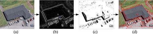
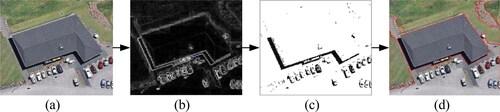
Figure 4. Segmentation results using Algorithm 1 (k = 5). (a) Original image; (b) Gradient image using Sobel operator; (c) Regional minimum image; (b) Segmentation result (k = 5).

2.2. Contour optimization driven by ground object contour algorithm and MDEDNet

2.2.1. Ground object contour optimization

The segmentation results presented in the previous subsection still have the following problems: (i) it is impossible to effectively measure the difference between objects due to the inconsistency within classes and ambiguity between classes, resulting in the multiline contour problem, as shown in Figure 5; (ii) the edge pixel classification and location of adjacent objects are unstable because the segmentation results depend too much on the gradient output of the structural edge algorithm and do not use semantic information of image depth, which leads to inaccurate contour locations, as shown in Figure 6.

Figure 5. Segmentation results obtained by MR-MAA-WS showing the problem of multiline contours. (a) Original image; (b) Segmentation results using MR-MAA-WS (k = 5); (c) Magnified view of segmentation result in upper left frame; (d) Magnified view of segmentation results in lower left frame.

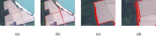
Figure 6. Segmentation results obtained by MR-MAA-WS showing the problem of inaccurate contour location. (a) Original image; (b) Segmentation results using MR-MAA-WS (k = 5); (c) Magnified view of segmentation result in upper right frame; (d) Magnified view of segmentation results in lower right frame.

Multiline contour optimization is adopted to address the multiline contour problem. The first step is to check the area covered by each label to ensure that each label in the image only covers one area. Preset structural elements are then used to ensure that the structural element traverses the whole image, eliminating regions smaller than the structural element. The specific steps are described in Algorithm 2.

Table

Algorithm 2: Ground Object Contour Optimization
Step 1: Ensure that each label in the image only covers one area;
Step 2: 1) Perform morphological opening operation on each tag region and subtract the opening operation result from the original image; Acquire an image $f_m$ after subtracting the opening operation; $f_m=U_{l=1}^L{b}_l-\delta \left(\epsilon \left(b_l\right)\right),$ in which $b_l$ is the first tag region, $l=1,2,...,L$ ;
Step 3: Reassign $f_m$ to adjacent areas, so that each area is labeled differently and re-labeled.

When applying Algorithm 2 to Figure 5, we obtain the results shown in Figure 7. Obviously, the proposed method addresses the problem of multiline contours without changing the shape of the segmented contour, but the problem of inaccurate contour positioning still exists.

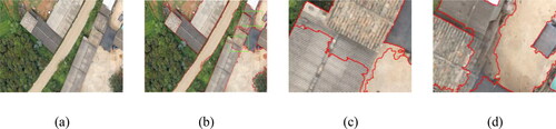
Figure 7. Multiline elimination results based on morphological contour optimization. (a) MR-MAA-WS segmentation result; (b) Ground object contour optimization result; (c) Contour optimization comparison in upper left frame; (d) Contrast results of contour optimization in lower left frame (line g represents the state before optimization and line y represents the state after optimization); (e) Legend.

2.2.2. Improved deep optimized ground object edge model

To improve the precision of segmentation and avoid the segmentation results from becoming over-dependent on the gradient, an image contour prediction model based on a CNN is introduced. The limitation of traditional neural network edge detection models lies in the lack of shallow detail information in deep feature information, which can easily prevent the network model from converging and cause the gradient to vanish (Liu and Lew 2016). Methods based on CNN architectures, such as DeepContour (Shen et al. 2015), richer convolutional features for edge detection (Liu et al. 2017), and holistically-nested edge detection (HED) (Xie and Tu 2015) offer significantly improved edge detection, but the continuous pooling layers still reduce the spatial resolution of features and lead to blurred edges (Cadieu et al. 2014). Additionally, the full convolution network architecture affects the similarity between adjacent edge pixels, making it impossible to capture the spatial positions accurately. In view of this, the crisp edge detector (CED) (Wang et al. 2019) network model has been proposed, which supplements the path details of the HED network. The CED model uses efficient subpixel convolution to gradually up-sample the pixel information, and improves the location accuracy of edge pixels. However, for high spatial resolutions with complex and changeable ground objects and prominent spatial details, the depth of the model network is insufficient and its accuracy is poor.

To overcome the aforementioned problems, an improved deep edge detection network is proposed. MDEDNet has a refined structure that enables detailed features of ground objects to be extracted in a hierarchical way, resulting in the output of accurate and clear edges. Specifically, each layer contains multiple optimization modules that use an edge coding process to output useful information. The network structure is shown in Figure 8.

Figure 8. Network structure diagram.

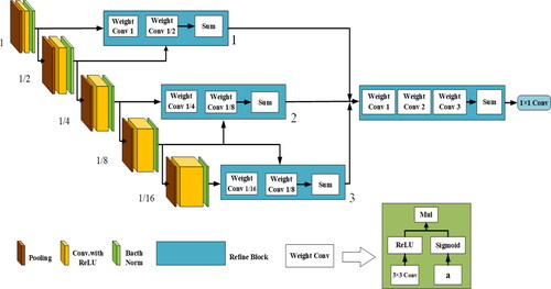
As can be seen from Figure 8, MDEDNet is an automatic encoder–decoder network based on a CNN architecture. The encoder part has five convolution layers with a core size of 3 × 3, and the pooling layers have a step size of 2 × 24. For an input image with a resolution of M × N, the final feature image resolution is (M/24) × (N/24).

The general optimization architecture is that of a top-down decoding network, allowing the fusion of multiple-resolution image output codes. The system is good at capturing hierarchical structure features, and can automatically fuse meaningful contours of ground objects at different stages. To fuse images with different resolutions, the MDEDNet structure extends the depth of the network horizontally to extract richer and more complex feature images, thus improving the universality of the model.

The core of MDEDNet is the Refine Block. The end-to-end task predicts the edge of the target from the high-resolution images. Based on the traditional CED network, the image features along the forward propagation path are added, and MDEDNet fuses the detailed results to obtain more accurate learning features. As the backbone, VGG-16 is used to optimize the module and restore the image feature resolution.

2.2.2.1. Connection

There are two types of connection methods in the Refine Block: skip connection and adjacent connection. The former receives characteristic images with a 4× resolution difference. For example, feature images with sizes of (1, 1/2), (1/4, 1/8) and (1/8, 1/16) on the left-hand modules in Figure 8 are used as inputs, and then, the low-resolution images are sampled to high-resolution images and fused with other high-resolution images. The adjacent left-hand module, as the input to three adjacent Refine Blocks, is the new Refine Block. The module fuses images of different resolutions by up-sampling each low-resolution part to the highest resolution part.

2.2.2.2. Refine block

The Refine Block includes up-sampling, point-by-point summation and weighted convolution layers. Because the feature images in each stage of the backbone network have different resolutions, bilinear up-sampling is used to up-sample the low-resolution feature images into high-resolution feature images. In addition, after connecting multiple input images, an element-by-element addition layer is used to fuse multiple inputs, rather than a 1 × 1 convolution layer. This is because element-by-element addition provides the best balance between performance and the number of training parameters. The output channel is set to the size of the minimum channel. After the last Refine Block, one convolution layer compresses the elements into one channel.

2.2.2.3. Weight convolution

The resolution of the image will affect the result of the final output boundary. Therefore, a weighted convolution layer is designed. The weighted convolution layer consists of two streams, one in the ReLU layer that applies 3 × 3 convolution and another using the sigmoid activation function to train the parameter α. The feature image obtained by the first stream is automatically weighted by the second stream. In the experiment, the weighted convolution layer should achieve higher performance at lower computational cost than the traditional convolution layer.

2.2.2.4. Loss function

For high-resolution remote sensing images, there is abundant information about the structure and texture of the ground objects, so it is difficult to segment the semantic boundary of ground objects. To address this problem effectively, the Dice coefficient is used to improve the fault tolerance of H and prevent over-fitting. The Dice loss function is (9) $$L(P,G)=\mathrm{Dist}(P,G)=\frac{{\sum }_i^n{p}_i^2+{\sum }_i^n{g}_i^2}{2{\sum }_i^n{p}_i{g}_i},$$(9) where $p_{i,\mathrm{ }}{g}_i$ are the values of the ith pixel on the segmented image P and the segmented real image G, respectively. The activated image M is the image processed by MDEDNet. The segmented image P is calculated from the activated image M by the sigmoid function. The loss function L is the reciprocal of the Dice coefficient. Because the Dice coefficient measures the similarity of two scenes, our loss term compares the similarity between the two groups of P and G. The loss of edge and non-edge pixels need not be taken into account, as long as the network is trained effectively and the edge of the ground object is clear. Thus, some training samples and corresponding ground conditions are selected in the experiment, and the total loss is calculated as (10) $$L\left(\mathrm{MP},\mathrm{ }\mathrm{MG}\right)={\sum }_I^M\mathrm{Dist}(\mathrm{M}{\mathrm{P}}_i,\mathrm{M}{\mathrm{G}}_i)\mathrm{ },$$(10) where MP and MG represent partially trained segmented samples and real segmented samples, respectively. M is the total number of partial training samples. To improve the performance of the model, the cross-entropy loss and Dice loss are combined. The Dice loss function focuses on the similarity of pixels in two scenes, whereas the cross-entropy loss function focuses on pixel-level differences. The combination of these two kinds of losses enhances the fault tolerance of MDEDNet and prevents over-fitting. The final loss function is written as (11) $$L_{\mathrm{final}}(P,G)=aL(P,G)+\tau L_c(P,G)\mathrm{ },$$(11) (12) $$L_c(P,G)=-\sum _j^N(g_j{p}_j+(1-g_j\left)\right(1-{\mathit{log}}_{p_j}\left)\right) ,$$(12) where $L(P,G)$ is the Dice loss function, $L_c(P,G)$ is the cross-entropy loss function, N is the total number of pixels in the image and $a,$ $\tau$ are the parameters of the two loss functions ($a$ = 1 and $\tau$ = 0.003 in our experiments). $L_{\mathrm{final}}(P,G)$ can be differentiated to obtain the gradient, as shown below: (13) $$\frac{\partial L_{\mathrm{final}}}{\partial g_k}=a\frac{2g_k\sum _{i=1}^N{p}_i{g}_i-g_k(\sum _{i=1}^N{p}_i^2+\sum _{i=1}^N{g}_i^2)}{2{\left(\sum _{i=1}^N{p}_i{g}_i\right)}^2}-\tau \frac{2g_k-1}{g_k},$$(13) where k is the calculated value of k pixels. The image gradient prediction results obtained by MDEDNet are shown in Figure 9(a); the original image is shown in Figure 6(a). The results show that MDEDNet can achieve better gradient prediction results with high-resolution spatial remote sensing images. When MR-MAA-WS is applied to Figure 9(a), the result still suffers from over-segmentation (see Figure 9(b)), but the contour fit is better than that without gradient prediction, as shown in Figure 9(c). Moreover, Figure 9(d,e) show magnified views of the regions in the rectangular boxes, where the yellow line y indicates the segmentation result after contour optimization and the green line g indicates the segmentation result before contour optimization. The comparison shows that MDEDNet helps the watershed transform to obtain more accurate contour location. Compared with MR-MAA-WS, MDEDNet creates over-segmentation but produces higher contour accuracy.

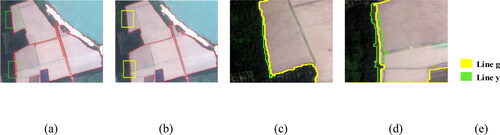
Figure 9. Segmentation results of joint MDEDNet and watershed algorithm. (a) Contour prediction result based on MDEDNet; (b) Segmentation results from MDEDNet and MR-MAA-WS; (c) MR-MAA-WS segmentation result; (d) Magnified view of contour optimization result in upper right frame; (e) Magnified view of contour optimization in lower right frame (line g represents the state before optimization and line y represents the state after optimization); (f) Legend.

Table

Algorithm 3: High-spatial-resolution remote sensing image segmentation result optimization using MDEDNet combined with MR-MAA-WS
Step 1: Input two images: 1) $f_{-\mathrm{mr}-\mathrm{maa}-\mathrm{ws}}$ (MR-MAA-WS segmentation result), 2) and ${\mathrm{ }f}_{-\mathrm{mdednet}}$ (MDEDNet segmentation result);
Step 2: Initialize: set value of m (total number of labels in the segmentation results based on MDEDNet);
Step 3: Define the label for ${\mathrm{ }f}_{-\mathrm{mdednet}}$ , where $i=1,\mathrm{ }2,\mathrm{ }...m$ ;
Step 4: Find the position L of label i in $f_{-\mathrm{mdednet}}$ ;
Step 5: Determine whether the label of L in $f_{-\mathrm{mr}-\mathrm{maa}-\mathrm{ws}}$ is ${\text{ label}}_{-\mathrm{mr}-\mathrm{maa}-\mathrm{ws}1}\mathrm{ },\mathrm{ }{\mathrm{label}}_{-\mathrm{mr}-\mathrm{maa}-\mathrm{ws}2}\mathrm{ },$…
Step 6: Select the label with the largest proportion from L and set it as ${\mathrm{label}}_{-\mathrm{mr}-\mathrm{maa}-\mathrm{ws}\mathrm{ }};$
Step 7: Output optimization result g.

3. Experiments and discussion

3.1. Dataset

At present, there is no published dataset for the edge segmentation of high-resolution remote sensing images, and all the published datasets are of natural scenery. Therefore, in addition to using the BSDS500 dataset containing 500 images (Arbeláez et al. 2011), 200 images were manually constructed for the experiments. The self-made images had a resolution of 500 × 500 pixels. Datasets for our experiments were composed of 280 training, 140 validation and 280 test images, with each image labelled by multiple annotators.

In our two-step training approach, we first train the base networks for the task of contour detection (coarse and fine). The network was implemented using PyTorch, an open-source machine learning library. For training, the hyperparameters of our model included: mini-batch size (10), global learning rate (0.01), learning rate decay (0.1) and weight decay (1 × 10⁻⁵). The trainable parameters a and τ were both set to 1. After the first step is finished, the weights of the base network are frozen, and the layers of the orientation subnetwork are connected and trained for an additional 6k iterations. Depending to the size of dataset we use different data augmentation strategies: flipping and rotation into 4 angles for self-made dataset; flipping, rotation into 16 angles for BSDS500. In all cases, we initialize the network from MDEDNet pretrained weights. The same ground-truth boundaries are used for training both the fine and the coarse contours.

To verify the effectiveness of the proposed method for high-resolution remote sensing images, three groups of images with a total of nine scenes are selected. The image information is presented in Table 1 and Figure 12, and the reference image is shown in Figure 13. The first group of three aerial remote sensing images come from the WuHan building dataset (I1, I2) (Ji et al. 2019) and the DOTA target detection dataset (I3) (Xia et al. 2018). The second group of three images (I4–I6) was taken by the domestic autonomous satellite Gaofen-2 (GF-2), and originate from the China Center for Resource Satellite Data and Applications (CRESDA). The third group of three stereo images come from reference (Xia et al. 2018) (I7) and Gaofen-7 (I8, I9), courtesy of CRESDA. The details are presented in Table 1.

Table 1. Information of segmentation dataset.

Grouping	Serial number	Source	Size	Resolution (m)
First	I1	WHU	872 × 543	0.3
	I2	WHU	2212 × 1882	0.3
	I3	DOTA	2806 × 1843	0.3
Second	I4	GF-2	1423 × 1495	4
	I5	GF-2	2387 × 2369	4
	I6	GF-2	2318 × 2406	4
Third	I7	DOTA	2172 × 1873	0.3
	I8	GF-7	958 × 565	0.8
	I9	GF-7	884 × 642	0.8

As shown in Figures 10 and 11, the nine images mainly include ground objects such as buildings, water bodies, vegetation, cultivated land and roads. The types of ground objects are complicated, with different shapes and complex spatial relations.

Figure 10. Original remote sensing images.

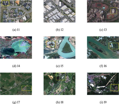
Figure 11. Reference images corresponding to original remote sensing images.

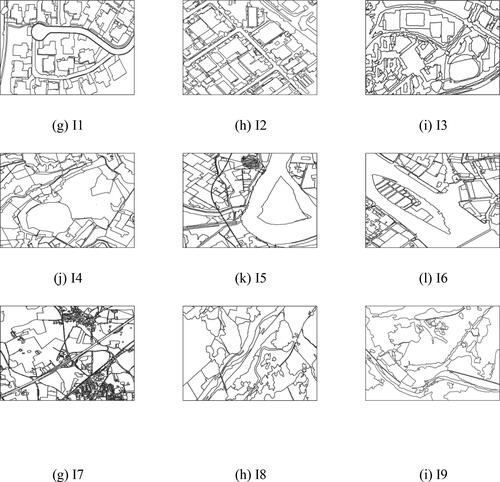
The first group of data contains dense areas of buildings, including residential houses, factories, office buildings and complex buildings. The building materials are complex, the roof color characteristics are rich, and the shapes are different. In I3, parts of the buildings are rendered in 3D stereo, and so the object textures and geometry information are more abundant and the homogeneity within the class is reduced. The second group of data shows mixed areas of water bodies, cultivated land and vegetation. There are many types of cultivated land, including paddy fields, irrigated land, cultivated land, fallow land and bare land. The internal texture structure is rich and the boundaries are fuzzy. The third group of data contains mixed areas of ground objects. The spatial relationship among the ground objects is more chaotic, the adjacency relationships are more complex and the scale of the ground objects varies, including linear rivers and roads, winding mountains, regular houses, cultivated land and irregular terraces.

3.2. Accuracy evaluation

To verify the accuracy of the experimental results, qualitative and quantitative methods are applied. The qualitative analysis compares the boundary adhesion, shape heterogeneity and the over- and under-segmentation of the segmented images. The quantitative analysis uses Eqs. (14)(14) $$R_u=1-\frac{B-C}{\mathrm{TP}+\mathrm{FP}},P_s=10\times {\log }_{10}{\left(\frac{\left(2^n-1\right)}{\mathrm{MSE}}\right)}^2\mathrm{ };$$(14) and (15)(15) $$P_r=\frac{\mathrm{TP}}{\mathrm{TP}+\mathrm{FP}}\mathrm{ },\mathrm{ }{R}_e=\frac{\mathrm{TP}}{\mathrm{TP}+\mathrm{FN}};$$(15) to compare and analyze the segmentation algorithms used in this article, with the actual boundaries of ground objects obtained by visual interpretation. (14) $$R_u=1-\frac{B-C}{\mathrm{TP}+\mathrm{FP}},P_s=10\times {\log }_{10}{\left(\frac{\left(2^n-1\right)}{\mathrm{MSE}}\right)}^2\mathrm{ };$$(14) (15) $$P_r=\frac{\mathrm{TP}}{\mathrm{TP}+\mathrm{FP}}\mathrm{ },\mathrm{ }{R}_e=\frac{\mathrm{TP}}{\mathrm{TP}+\mathrm{FN}};$$(15) where R_u is the regional gray consistency; P_s is the peak signal-to-noise ratio; B and C are the regional gray variance and regional binary variance, respectively; MSE is the root mean square error; P_r is the segmentation accuracy (Shen et al. 2020); R_e is the boundary recall rate (Hou et al. 2020); TP is the sample number of the result pixels for which the ground object is correctly segmented; FP is the sample number of the segmentation result for which the background pixels are divided into ground object pixels; and FN is the number of samples divided into background pixels.

The experiments were performed on a Windows 10 platform with an Inter(R) Core(TM) i7-10700 2.9 GHz CPU and 16 GB RAM. All algorithms and experimental evaluations were implemented in MATLAB 2018b, except for the Fractal Net Evolution Approach (FNEA) algorithm [38], which was implemented in eCognition Developer.

3.3. Results

To verify the effectiveness of the proposed method, eight algorithms were selected for comparative analysis, namely, the Watershed Algorithm (WS) (Zhang and Zhang 2017), Simple Linear Iterative Clustering (SLIC) (Achanta et al. 2012); Mean Shift (MS) (Comaniciu and Meer 2002); Linear Spectral Clustering (LSC) (Chen et al. 2017); FNEA (Huang and Zhang 2009); Sobel with Morphological Gradient Reconstruction-based Watershed Algorithm (Sobel-MGR-WS) (Cui et al. 2014); SE with adaptive Morphological Reconstruction and Watershed Algorithm (SE-AMR-WS) (Lei et al. 2019); and Sobel with adaptive Morphological Reconstruction and Watershed Algorithm (Sobel-AMR-WS) (Huang et al. 2020).

3.3.1. Test results of first set of data

3.3.1.1. Qualitative evaluation

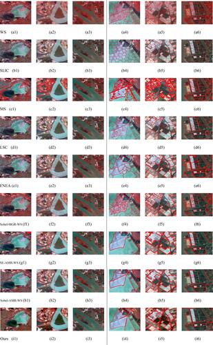
To evaluate the segmentation results, aerial remote sensing images I1–I3 were segmented in experiment 1. The results are shown as follows. To facilitate visual comparison, partial areas are locally enlarged on the right side of the black vertical line in Figure 12.

Figure 12. Comparison of group one segmentation results.

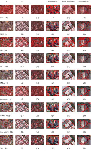
Figure 12 shows the segmentation result for the first group of experimental images, where each column in the figure represents an experimental image and each row represents an algorithm. As we can see, group-1 images show building-dense areas, with complex building types and sizes and rich roof colors and texture structures. Image I3 is a 3D building area, in which surrounding objects may be easily confused, increasing the difficulty of segmentation.

Figure 12(a) shows the WS segmentation result. The segmentation effect of this algorithm is related to the image gradient and seed point selection. Points at which the gradient less than 3 are used as seed points in the experiments. However, the texture structure of the buildings in the image is rich, and the initial seed points are sensitive to noise, which results in serious over-segmentation.

Figure 12(b) is the experimental result from the SLIC algorithm using 500 super-pixels. SLIC is a super-pixel algorithm based on k-means clustering. The objective function is mapped to the CIELAB color space and distance space, as this retains local spatial information and has better adaptability to high-resolution remote sensing images with complex backgrounds. Compared with the WS method, the boundary adhesion is improved. However, the super-pixel blocks are uniform in size and regular in shape, which is good for buildings of regular sizes, but produces a poor fit for vegetation boundaries with irregular shapes. Thus, SLIC is not suitable for these experimental images.

Figure 12(c) is the segmentation result obtained by the MS algorithm with a segmentation threshold of 0.6, which provides a good expression of the spectral characteristics of ground objects. For example, in Figure 12(c5), the boundary between the white buildings and roads is obvious, the integrity of ground objects is optimized, and there are few broken areas. However, the MS algorithm struggles to distinguish complex ground objects, and the adhesion rate of boundaries is poor, leading to fuzzy edges around ground objects and serious multicontour occurrences.

Figure 12(d) is the segmentation result of LSC. Compared with the first three methods, the results obtained by this method are more accurate in positioning ground objects, and the contour fit is obviously improved. This is because LSC uses undirected weight maps to form adjacent matrices for clustering, and has stronger adaptability to complex scenes. However, the method is affected by illumination, resulting in segmentation errors. For example, in the blue roof in Figure 12(d4), the illumination produces different areas with different brightness values, which leads to serious over-segmentation. However, the spectral homogeneity of the white roof in Figure 12(d6) is very high, and the texture difference is not obvious, resulting in a very good segmentation effect.

Figure 12(e) is the segmentation result of FNEA. The segmentation method comprehensively utilizes spectrum, shape, texture and other information to segment the image into homogeneous regions with similar features, resulting in more natural segmentation objects that are close to the real ground object boundaries. In the experiments, the shape heterogeneity and compactness parameters were fixed at 0.7 and 0.5, respectively. Because of the great difference in the size of the experimental images, there was no fixed scale and so an interval of 60–140 was examined in steps of 20. Considering the uncertainty of homogeneous region features, this method enhances the uncertainty expression of pixel categories, thus, optimizing the boundary segmentation effect. This ensures the accuracy of the segmentation results to a certain extent, and makes the size and shape of ground object segmentation more consistent with the reference images. However, this method requires a number of parameters to be set and considerable processing work, resulting in a low degree of automation.

Figure 12(f) is the segmentation result of the algorithm Sobel-MGR-WS,which is denoted by SMW in Tables 2–4. Sobel-based gradient reconstruction and the morphological watershed algorithm are used to complete the segmentation, and the image noise is obviously suppressed. The single-scale structural elements are used to reconstruct the gradient image, and so ground objects of different sizes cannot be accounted for, so over-segmentation remains a problem and there are many scattered small patches. For example, in Figure 12(f2), the segments of large-sized buildings and roads are relatively broken. In addition, in highly textured vegetation areas, highly irregular segmentation results are presented: the vegetation segmentation boundaries are unclear, leading to serious multiline contour problems.

Table 2. Quantitative results (R_u, P_s, P_r, R_e and T_ime) for the first group of images.

Dataset		Method
		WS	SLIC	MS	LSC	FNEA	SMW	SAW	SoAW	Ours
I1	Ru	0.7434	0.7779	0.7842	0.7639	0.7558	0.7352	0.8365	0.8536	0.8963
	Ps	31.8950	32.3210	31.9560	32.2560	32.0230	31.9520	32.8420	31.2360	32.9950
	Pr	0.8015	0.7568	0.8013	0.8153	0.7856	0.8536	0.8126	0.8354	0.8869
	Re	0.8632	0.8521	0.8671	0.8742	0.8532	0.8812	0.8752	0.8635	0.9012
	Time	6.8900	7.5300	6.5300	6.7600	6.8400	7.2200	7.3200	7.5300	6.1900
I2	Ru	0.7232	0.7485	0.7195	0.7587	0.7158	0.8136	0.8586	0.7953	0.8833
	Ps	31.9950	32.0840	31.9540	31.8630	31.8600	32.3570	31.2560	31.9960	32.5540
	Pr	0.8236	0.7958	0.8102	0.8356	0.8012	0.8785	0.8563	0.8536	0.8799
	Re	0.8589	0.8369	0.8544	0.8812	0.8612	0.8762	0.8589	0.8698	0.8966
	Time	6.9600	7.8300	6.5500	6.7400	6.9200	7.0100	7.5300	7.4600	6.7300
I3	Ru	0.7536	0.7324	0.7123	0.8042	0.7564	0.8365	0.8256	0.8555	0.8988
	Ps	31.8540	32.3250	32.0840	32.2460	31.9850	31.2370	32.5420	31.9860	32.5560
	Pr	0.8256	0.8345	0.7988	0.8532	0.7932	0.8362	0.8025	0.8785	0.8922
	Re	0.8688	0.8595	0.8521	0.8470	0.8422	0.8722	0.8698	0.8725	0.8953
	Time	6.9800	7.6300	6.7800	6.8600	7.2300	7.2200	7.2600	7.2100	6.7900

Larger values are better. The best values are indicated in bold.

Table 3. Quantitative results (R_u, P_s, P_r, R_e and T_ime) for the second group of images.

Dataset		Method
		WS	SLIC	MS	LSC	FNEA	SMW	SAW	SoAW	Ours
I4	Ru	0.7386	0.8012	0.7721	0.8236	0.7238	0.8558	0.8463	0.8756	0.8831
	Ps	31.5360	32.4210	31.5370	32.5550	32.0360	31.9850	32.5240	32.4860	32.7520
	Pr	0.7553	0.7521	0.7526	0.7856	0.8125	0.8123	0.8126	0.8354	0.8769
	Re	0.8588	0.8632	0.8600	0.8577	0.8326	0.8810	0.8792	0.8711	0.8896
	Time	6.9800	7.2100	7.4600	7.5300	7.2400	7.3600	6.9900	7.2300	6.6800
I5	Ru	0.7325	0.7512	0.8140	0.7958	0.7222	0.8532	0.8756	0.8752	0.9123
	Ps	32.2360	32.1260	32.5630	32.5240	32.2570	32.7790	32.8900	32.4850	32.9360
	Pr	0.7741	0.7368	0.7513	0.7153	0.7841	0.7936	0.8226	0.8754	0.8977
	Re	0.8588	0.8732	0.8456	0.8712	0.8498	0.8785	0.8752	0.8750	0.8830
	Time	7.1200	7.5600	6.9900	7.2100	7.5400	7.3300	7.5400	7.6800	6.7200
I6	Ru	0.7365	0.7216	0.7536	0.7124	0.7547	0.8002	0.8356	0.8412	0.8758
	Ps	31.9860	32.2560	32.5630	32.4990	32.2370	32.3270	32.5370	32.8650	32.7800
	Pr	0.7563	0.7896	0.7521	0.8236	0.7563	0.8036	0.8026	0.7896	0.8326
	Re	0.8532	0.8421	0.8563	0.8624	0.8423	0.8724	0.8755	0.8721	0.8839
	Time	7.1900	7.6300	7.5300	7.2600	7.5900	7.2100	7.3600	7.5500	6.9800

Larger values are better. The best values are indicated in bold.

Table 4. Quantitative results (R_u, P_s, P_r, R_e and T_ime) for the third group of images.

Dataset		Method
		WS	SLIC	MS	LSC	FNEA	SMW	SAW	SoAW	Ours
I7	Ru	0.7445	0.7298	0.7546	0.7623	0.7445	0.8535	0.8244	0.8586	0.8842
	Ps	31.9860	31.8540	31.8540	31.2540	32.2370	32.054	32.0240	31.9940	32.3680
	Pr	0.7362	0.7421	0.7863	0.8013	0.7532	0.7826	0.8011	0.8321	0.8669
	Re	0.8495	0.8499	0.8572	0.8592	0.8455	0.8547	0.8637	0.8693	0.8733
	Time	7.6800	7.7800	7.5300	7.4400	7.5900	7.6300	7.4800	7.8300	7.2100
I8	Ru	0.7586	0.7321	0.7123	0.7239	0.7499	0.7985	0.8203	0.8536	0.8777
	Ps	31.5500	32.2360	31.5440	32.6620	31.8540	31.2850	32.3960	31.4470	32.7540
	Pr	0.7015	0.7168	0.6913	0.6842	0.7253	0.7236	0.7926	0.8054	0.8355
	Re	0.8632	0.8521	0.8671	0.8742	0.8532	0.8812	0.8752	0.8635	0.9012
	Time	7.5900	7.6300	7.8200	7.4600	7.5700	7.6600	7.5300	7.7900	7.1900
I9	Ru	0.7314	0.7853	0.7763	0.7513	0.7256	0.8366	0.8572	0.8110	0.8233
	Ps	31.8690	31.5370	31.5340	32.0390	32.3270	31.3850	32.0030	31.9810	32.5530
	Pr	0.6515	0.6968	0.6413	0.7153	0.7023	0.7536	0.7326	0.7554	0.7893
	Re	0.8123	0.8055	0.8632	0.8614	0.8325	0.8722	0.8632	0.8236	0.9032
	Time	7.7800	7.7300	7.9900	7.6200	7.6000	7.7400	7.6600	7.8300	7.4500

Larger values are better. The best values are indicated in bold.

Figure 12(g) is the segmentation result of the SE-AMR-WS method, which is denoted by SAW in Table 2.3.4, and guarantees both monotonic increments and convergence. Compared with Sobel-MGR-WS, the adaptive multiscale morphological operator is used to reconstruct the gradient in this method. The reconstruction effect is better than that of single-scale gradient reconstruction, as the problem of over-segmentation is addressed. Thus, the integrity of building and road segmentation is improved, the smoothness and fit of the boundary are obviously better, and the false segmentation of vegetation is suppressed. Overall, the segmentation accuracy is obviously improved. However, adjacent objects with little difference in spectrum and texture still suffer from under-segmentation, as shown in Figure 12(g3). Hence, this algorithm is not suitable for the images used in this experiment.

Figure 12(h) is the segmentation result of Sobel-AMR-WS, which is denoted by SoAW in Table 2.3.4. These results are similar to those of SE-AMR-WS, but the segmentation of some large-scale buildings are more accurate. Although the segmentation results of SE-AMR-WS have a high coincidence rate with the reference images, they do not form an independent closed area. In contrast, the segmentation regions obtained by Sobel-AMR-WS are closed and independent of each other, and the segmentation accuracy is further improved. However, the problem of image over-segmentation has not been well addressed. As shown in Figure 12(h1), the blue roof is over-segmented due to the uneven light and shade changes. The interior texture details of the white building in Figure 12(h3) are prominent and need to be further merged and clustered.

Figure 12(i) is the segmentation result of the proposed MDEDNet-MR-MAA-WS method. Compared with the other algorithms, this method is accurate for ground object segmentation. The details of the inner areas of building surfaces are well aggregated, and the segmentation presents regular rectangles. At the same time, some positions with fuzzy boundaries are accurately segmented without multiple segmentation blocks, and the boundaries of small areas of vegetation are completely preserved. Additionally, the problem of double-line contours is adequately addressed. In terms of both qualitative visual contrast and quantitative precision, the proposed method achieves the best segmentation effect.

3.3.1.2. Quantitative evaluation

The metrics of R_u, P_s, P_r and R_e were used to evaluate the segmentation results. The results are presented in Table 2 and Figure 13.

Figure 13. Performance comparison of different algorithms on the first group of data.

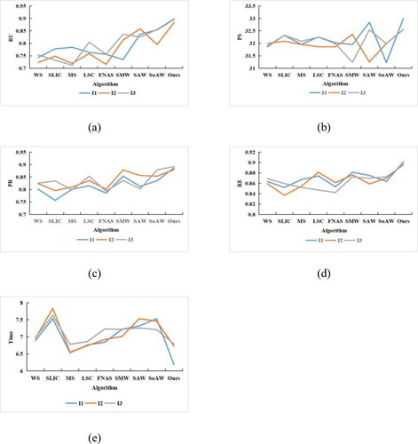
As can be seen from Table 2 and Figure 13, WS is not suitable for these experimental images, and the scores of the various evaluation indexes are not high. SLIC, MS and FNEA give a higher segmentation accuracy and higher boundary repetition rate than WS, but the regional gray consistency does not score highly. Although Sobel-MGR-WS adds morphological operators to improve the gradient images, the optimization effect is not obvious for high-resolution remote sensing images. SE-AMR-WS and Sobel-AMR-WS offer significant improvements in each index, which shows that the adaptive morphological reconstruction operator allows better adaptation to the feature distribution of various ground objects in the experimental images, but there is still insufficient segmentation of individual objects. Compared with the other algorithms, the proposed method obtains the highest experimental index scores, which shows that it achieves better performance in terms of ground object segmentation. Compared with the experimental results for I2 and I3, the segmentation effect of I1 is the best. This is mainly because the internal spectral details of ground objects in I1 are simple, the boundaries are obvious and the contours are single and easy to distinguish.

3.3.2. Test results of second set of data

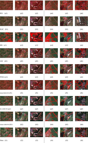
3.3.2.1. Qualitative evaluation

Figure 14 shows the segmentation result of the second group of experimental images. This group of images mainly shows mixed areas of water, cultivated land and vegetation. The intraclass details are highly textured, the differences between classes become lower, and the boundaries are blurred, which increases the difficulty of segmentation.

Figure 14. Comparison of group two segmentation results.

Figure 14(a) is the segmentation result of the WS method. The segmentation effect is relatively good for water areas with high internal homogeneity, although the over-segmentation of other cultivated land areas is still very serious. Figure 14(b) shows the segmentation result of the SLIC method. As SLIC is not affected by changes in texture features, the segmentation effect of Figure 14(b) is similar to that of Figure 12(b).

Figure 14(c) shows the segmentation result of the MS method. Under the weaker influence of spectral differences, the segmentation shape of the MS method is the most regular and complete in water areas and some paddy field areas with low brightness values. However, at the boundaries between water and land, the problem of multicontour lines becomes serious, as shown in Figure 14(c1). This is because the spectrum and texture are very similar, the distribution is dense, the shape is extremely irregular, and the boundary is not obvious. These factors make the segmentation difficult. In addition, there are many small fragments in the highlighted cultivated land areas with prominent texture details inside the ground objects, as shown in Figure 14(c2).

Figure 14(d) is the segmentation result of the LSC method. Compared with MS, the LSC algorithm improves the over-segmentation to a certain extent, but the segmentation boundaries in some edge areas are fuzzy, even producing ‘pseudo boundaries’. Therefore, this method does not meet the target segmentation accuracy requirements.

Figure 14(e) is the segmentation result of the FNEA algorithm, which is optimized to express the texture information between ground objects. Compared with LSC, the obtained segmentation boundaries are smoother and more natural, especially for the uncertain texture features in highlighted cultivated land areas. Therefore, the size and shape of ground object segmentation is more consistent with the reference images. However, a large number of multiline boundaries inevitably appear when using this method. The reason may be that the spectral heterogeneity between adjacent objects in this group of data is lower and the distribution of objects is denser and more complex, which leads to fuzzy segmentation boundaries, making it difficult to accurately segment the experimental images.

Figure 14(f) shows the segmentation result of Sobel-MGR-WS. Compared with the WS segmentation results, the over-segmentation situation has been improved for some small cultivated land areas in which the details of ground objects are very clear, and regular rectangles appear at the beginning of the segmentation. However, for densely distributed cultivated land areas, the segments still contain a lot of noise.

Figure 14(g) present the segmentation result of the SE-AMR-WS method. Although the boundary between irrigated fields and water bodies is under-divided, as shown in Figure 14(g3), fallow farmland, highlighted farmland and bare land are better aggregated, and the segmentation contours of various ground objects are smoother. This means that important target contour information is retained, allowing the segmentation results to reflect the surface features of ground objects to a certain extent. These factors indicate that this method is closer to the ideal segmentation effect.

The segmentation result of the Sobel-AMR-WS method, shown in Figure 14(h), is similar to those of SE-AMR-WS, albeit with stronger recognition, less under-segmentation and higher overall segmentation accuracy for ground objects with less obvious internal details and lower spectral differences. However, a small number of ground objects with inconspicuous boundaries have offset segmentation boundaries. This method partially suppresses the phenomenon of over-segmentation.

Figure 14(i) is the segmentation result of the proposed method. From the perspective of segmentation accuracy and visual effect, this method gives the optimal segmentation, and the details of the internal areas of different types of cultivated land surface are clearly segmented. The segmentation produces regular rectangles, as shown in Figure 14(j2), which completely retain the target contour information of small areas such as irrigated fields and mixed cultivated land. In addition, in terms of the positions where the spectrum and texture of adjacent objects are similar and the boundary is more blurred, the proposed method produces accurate segmentation, and the multiline contour problem is properly addressed (e.g. the boundary between irrigated land and water body in Figure 14(j1,j3)). In summary, the method proposed in this article gives the best segmentation results, which are in good agreement with the boundaries of the corresponding reference images.

3.3.2.2. Quantitative evaluation

The metrics of R_u, P_s, P_r and R_e were used to evaluate the segmentation accuracy. The results are presented in Table 3 and Figure 15.

Figure 15. Performance comparison of different algorithms on the second group of data.

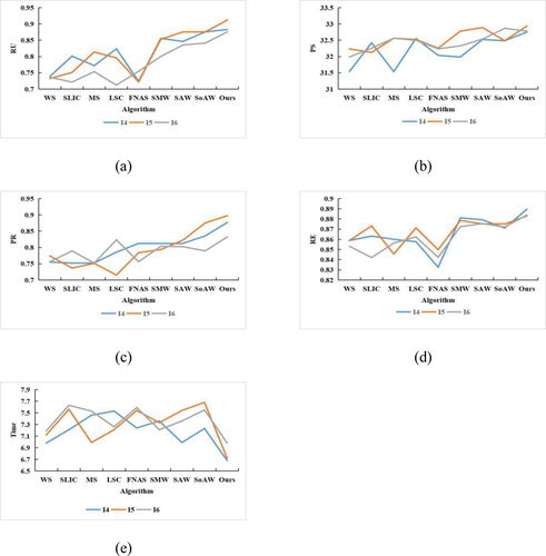
According to the segmentation evaluation results in Table 3 and Figure 15, the four index values are slightly lower for the second group of images than for the first group. These values may have been affected by the increase in the experimental map area and the associated increase in the complexity of ground objects. The factors that affect the accuracy of image segmentation include regional resolution, the range of the segmented region, the distribution of ground objects and the accuracy of boundaries. Another important factor is the diversification of cultivated land types. Although cultivated land has the same ground objects in different periods and different functions, its spectral, texture and spatial characteristics are extremely similar but slightly different, its intraclass heterogeneity is further increased, and its texture structure is more complex. Thus, it is more difficult to perform segmentation. Overall, compared with the other experimental methods, the proposed method gives the highest P_r, R_u, P_s and R_e values, which fully proves the applicability of the proposed method.

3.3.3. Test results of third set of data

3.3.3.1. Qualitative evaluation

Figure 16 shows the segmentation result of the third group of experimental images, where each column represents an experimental image and each row represents an algorithm. The third group of data consists of multitype mixed area ground objects, where the spatial relationship between the ground objects is chaotic, the adjacency relationships are complex and the scale difference of ground objects is large. Each of these factors makes the segmentation more difficult.

Figure 16. Comparison of group three segmentation results.

The WS method produces serious mis-segmentation and over-segmentation, as shown in Figure 16(a2). Water and vegetation are mistakenly segmented together, a result of the highly detailed spectral and texture structures of high-resolution remote sensing images, and the subtle differences among the features of adjacent ground objects. The closer the staggered distribution of any two adjacent objects, the more serious is the mis-segmentation. SLIC produces poor adhesion at the boundary of this group of experimental images, with a failure to correctly reflect the shape characteristics of ground objects. The main reason is that the types of ground objects are too complex, their geometric shapes are quite different, and the internal organization structure is rich, such as linear rivers and roads, rectangular residential areas, irregular lakes and vegetation. This method cannot account for the complex distribution characteristics of ground objects in remote sensing images, so the segmentation accuracy drops significantly. The MS method still suffers from over-segmentation and unclear segmentation boundaries. The smaller the scale of the ground objects, the more broken is the segmentation. Compared with MS, the boundary definition of the LSC method is better, but when dealing with the same type of ground objects with obvious spectral differences, it suffers from over-segmentation, resulting in many broken small patches. This leads to non-smooth segmentation boundaries, as shown in Figure 16(d2,d3). The overall segmentation effect of the FNEA method is better than that of the abovementioned methods. In building areas with inconspicuous boundaries and vegetation areas with high texture gradients, FNEA produces accurate and smooth segmentation contours and correctly reflects the shape characteristics of various objects, but the over-segmentation problem has not been properly addressed. Compared with the previous two sets of experimental images, the over-segmentation problem has become more serious with the Sobel-MGR-WS method, which cannot even recognize the attribute of the building area in Figure 16(f3), and cannot generate an independent and complete segmentation block containing this area. The segmentation results of the SE-AMR-WS and Sobel-AMR-WS methods are similar, with well-preserved regular large-scale features of ground objects, but the segmentation of irregular ground objects and small ground objects, such as flowing rivers and rectangular residential buildings, is generally poor, and the segmentation accuracy is insufficient.

The proposed method is optimal in terms of both the visual effect and segmentation accuracy. In the segmentation region where the boundary is not obvious and the spectrum is approximate, the spectrum of the grassland boundary area is very close to that of the water body, and the problem of false segmentation is obviously suppressed, which results in higher accuracy. The proposed method is optimal because it combines the adaptive gradient reconstruction operator with minimum region deletion and the deep learning boundary prediction model. This results in an accurate fit of the distribution characteristics of various objects, full expression of the shape characteristics of different types of ground objects, and accurate segmentation of some positions with fuzzy boundaries. Thus, the proposed method effectively addresses the false segmentation caused by the phenomenon of ‘different objects with the same spectrum and different spectra with the same object’ in remote sensing images, indicating that it can correctly segment high-resolution remote sensing images.

3.3.3.2. Quantitative evaluation

The metrics of R_u, P_s, P_r and R_e were used to accurately evaluate the segmentation accuracy. The results are presented in Table 4 and Figure 17.

Figure 17. Performance comparison of different algorithms on the third group of data.

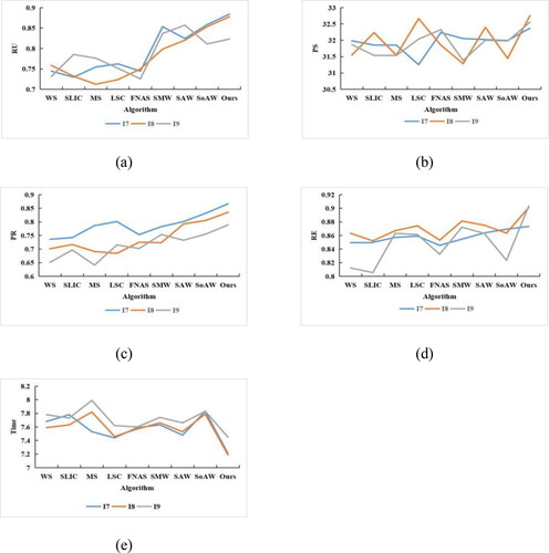
As can be seen from Table 4 and Figure 17, when the map width, ground object type, spatial distribution, image resolution and contour complexity are increased at the same time, the traditional methods all give poor segmentation accuracy. SE-AMR-WS and Sobel-AMR-WS make use of the self-adaptive segmentation threshold, which leads to stable and less affected results. In summary, the evaluation indexes of the three groups of experimental images decrease as the segmentation difficulty of high-resolution remote sensing images increases. However, compared with other algorithms, the proposed method maintains higher values of the evaluation metrics. From the above analysis, it can be concluded that the visual effect of segmentation results is consistent with the experimental indexes, and the segmentation effect of MR-MAA-WS combined with MDEDNet is better than that of existing techniques.

4. Conclusion

This article has described a method that combines the minimum area adaptive watershed transform based on morphological reconstruction with a modified deep edge detection network. MR-MAA-WS reconstructs the gradient features of the image and performs watershed segmentation to obtain the initial segmentation results. A ground object contour optimization method and MDEDNet further improve the accuracy of the segmented image. Experiments on three groups of images have demonstrated that the segmentation accuracy is improved by our method, enabling the accurate segmentation of high-spatial-resolution remote sensing images.

However, due to the high resolution and rich texture information of such images, the segmentation accuracy of MDEDNet depends on the number of training samples. To address this problem, future work will focus on weak supervised learning and the use of generative adversarial networks to improve the generalization ability and efficiency of the proposed method.

Author’s contributions

Acquisition of the financial support for the project leading to this publication, Z.Y. and L.H. Application of statistical, mathematical, computational or other formal techniques to analyze or synthesize study data, H.N., Z.Y., D.X. and X.W. Preparation, creation and/or presentation of the published work by those from the original research group, specifically critical review, commentary or revision, including pre- or post-publication stages, H.N., J.S. and Z.Y.

Disclosure statement

No potential conflict of interest was reported by the authors.

Data availability statement

The code used in this study are available by contacting the corresponding author.

Additional information

Funding

Project supported by the National Natural Science Foundation of China, grant number 41371524, Scientific and Technological Innovation Team of Universities in Henan Province, grant number 22IRTSTHN008.

References

- Abdollahi A, Pradhan B, Alamri A. 2021. RoadVecNet: a new approach for simultaneous road network segmentation and vectorization from aerial and Google earth imagery in a complex urban set-up. Gisci Remote Sens. 58(7):1151–1174.
- Achanta R, Shaji A, Smith K, Lucchi A, Fua P, Süsstrunk S. 2012. SLIC superpixels compared to state-of-the-art superpixel methods. IEEE Trans Pattern Anal Mach Intell. 34(11):2274–2282.
- Achanta R, Susstrunk S. 2017. Superpixels and Polygons Using Simple Non-iterative Clustering. IEEE Conf Comput Vis Pattern Recognit. p. 4895–4904.
- Arbeláez P, Maire M, Fowlkes C, Malik J. 2011. Contour detection and hierarchical image segmentation. IEEE Trans Pattern Anal Mach Intell. 33(5):898–916.
- Awaisu M, Li L, Peng J, Zhang J. 2019. Fast superpixel segmentation with deep features. Adv Comput Graph. p. 410–416
- Bai Y, Chen X. 2016. Efficient structure-preserving superpixel segmentation based on minimum spanning tree. IEEE International Conference on Multimedia and Expo. p. 1–6.
- Biswajeet P, Husam AHA, Maher IS, Ivor T, Abdullah MA. 2020. Unseen land cover classification from high-resolution orthophotos using integration of zero-shot learning and convolutional neural networks. Remote Sensing. 12(10):1676.
- Cadieu C, Hong H, Yamins D, Pinto N, Ardila D, Solomon E, Majaj N, DiCarlo J. 2014. Deep neural networks rival the representation of primate IT cortex for core visual object recognition. PLoS Comput Biol. 10(12):e1003963.
- Chen J, Li Z, Huang B. 2017. Linear spectral clustering superpixel. IEEE Trans Image Process. 26(7):3317–3330.
- Comaniciu D, Meer P. 2002. Mean shift: a robust approach toward feature space analysis. IEEE Trans Pattern Anal Machine Intell. 24(5):603–619.
- Cui X, Y. Deng G, Yang G, Wu S. 2014. An improved image segmentation algorithm based on the watershed transform. IEEE 7th Joint International Information Technology and Artificial Intelligence Conference. p. 28–431.
- Deng L, Geoffrey H, Brian K. 2013. New types of deep neural network learning for speech recognition and related applications: an overview. International Conference on Acoustics, Speech, and Signal Processing. p. 26–31.
- Deng R, Shen C, Liu S, Wang H, Liu X. 2018. Learning to predict crisp boundaries. Comput Vis Pattern Recognit. 11210:562–578.
- Drever L, Roa W, McEwan A, Robinson D. 2007. Iterative threshold segmentation for PET target volume delineation. Med Phys. 34(4):1253–1265.
- Fan Y, Chen W, Pan Z. 2008. An adaptive watermarking algorithm in DWT domain based on multi-scale morphological gradient. Int Conf Comput Sci Softw Eng. p. 738–741.
- Fang Z, Yu X, Wu C, Chen D, Jia T. 2018. Superpixel segmentation using weighted coplanar feature clustering on RGBD images. Appl Sci. 8(6):902.
- Farabet C, Couprie C, Najman L, Lecun Y. 2013. Learning hierarchical features for scene labeling. IEEE Trans Pattern Anal Mach Intell. 35(8):1915–1929.
- Hou M, Yin J, Ge J, Li Y, Feng Q. 2020. Land cover remote sensing classification method of alpine wetland region based on random forest algorithm. Trans Chin Soc Agric Machinery. 51:220–227.
- Huang L, Yao B, Chen P, Ren A, Xia Y. 2020. Superpixel segmentation method of high resolution remote sensing images based on hierarchical clustering. J Infrared Millim Waves. 39:263–272.
- Huang X, Zhang L. 2009. A comparative study of spatial approaches for urban mapping using hyperspectral ROSIS images over Pavia City, northern Italy. Int J Remote Sens. 30(12):3205–3221.
- Huo F, Yang L, Wang D, Sun B. 2017. Bloch quantum artificial bee colony algorithm and its application in image threshold segmentation. Signal Image Video Process. 11:1–8.
- Ji S, Wei S, Lu M. 2019. Fully convolutional networks for multi-source building extraction from an open aerial and satellite imagery dataset. IEEE Trans Geosci Remote Sensing. 57(1):574–586.
- Lei T, Jia X, Liu T, Liu S, Meng H, Nandi AK. 2019. Adaptive morphological reconstruction for seeded image segmentation. IEEE Trans Image Process. 28(11):5510–5523.
- Lei T, Jia X, Zhang Y, Liu S, Meng H, Nandi AK. 2019. Superpixel-based fast fuzzy C-means clustering for color image segmentation. IEEE Trans Fuzzy Syst. 27(9):1753–1766.
- Li C, Zhao L, Sun S. 2010. An adaptive morphological edge detection algorithm based on image fusion. 3rd International Congress on Image and Signal Processing. p. 1072–1076.
- Liu Y, Cheng M, Hu X, Wang K, Bai X. 2017. Richer convolutional features for edge detection. IEEE Conf Comput Vis Pattern Recognit. p.5872–5881.
- Liu Y, Lew MS. 2016. Learning relaxed deep supervision for better edge detection. IEEE Conf Comput Vis Pattern Recognit. p.231–240.
- Long J, Shelhamer E, Darrell T. 2014. Fully convolutional networks for semantic segmentation. IEEE Trans Pattern Anal Mach Intell. 39:640–651.
- Mahaman SC, Pierre-Henri C, Karim K, Basel S, Mohamed AM. 2017. Adaptive strategy for superpixel-based region-growing image segmentation. J Electron Imaging. 26:1.
- Nakamura K, Byung-Woo H. 2016. Fast-convergence superpixel algorithm via an approximate optimization. J of Electron Imag. 25(5):053035.
- Rémi G, Vinh T, Nicolas P. 2018. Robust superpixels using color and contour features along linear path. Comput Vision Image Understanding. 170:1–13.
- Ren X, Malik J. 2003. Learning a classification model for segmentation. Proceedings Ninth IEEE International Conference on Computer Vision.p. 10–17.
- Rother C, Kolmogorov V, Blake A. 2004. GrabCut: interactive foreground extraction using iterated graph cuts. ACM Trans Graph. 23(3):309–314.
- Shen J, Hao X, Liang Z, Yu L, Wang W, Shao L. 2016. Real-time superpixel segmentation by DBSCAN clustering algorithm. IEEE Trans on Image Process. 25(12):5933–5942.
- Shen W, Wang X, Wang Y, Bai X, Zhang Z. 2015. Deepcontour: a deep convolutional feature learned by positive-sharing loss for contour detection. IEEE Conf Comput Vis Pattern Recognit. p. 3982–3991.
- Shen Y, Yuan Y, Peng J, Chen X, Yang Q. 2020. River extraction from remote sensing images in cold and arid regions based on deep learning. Trans Chin Soc Agric Machinery. 51:192–201.
- Sun JG, Liu J, Zhao LY. 2008. Clustering algorithms research. J Softw. 19(1):48–61.
- Wang Y, Zhao X, Li Y, Huang K. 2019. Deep crisp boundaries: from boundaries to higher-level tasks. IEEE Trans Image Process. 28(3):1285–1298.
- Wu MY, Chen L. 2015. Image recognition based on deep learning. Chinese Automation Congress. p. 27–29.
- Xia G, Bai X, Ding J, Zhu Z, Belongie S, Luo J, Datcu M, Pelillo M, Zhang L. 2018. DOTA: a large-scale dataset for object detection in aerial images. 2018 IEEE/CVF Conference on Computer Vision and Pattern Recognition.
- Xie S, Tu Z. 2015. Holistically-Nested Edge Detection. IEEE International Conference on Computer Vision. p. 1395–1403.
- Xu G, Su Z, Wang J, Yin Y, Shen Y. 2008. An adaptive morphological filter based on multiple structure and multi-scale elements. Int Conf Comput Sci Softw Eng. p. 399–403.
- Yamini B, Sabitha R. 2017. Image steganalysis: adaptive color image segmentation using otsu’s method. J Comput Theor Nanosci. 14(9):4502–4507.
- Yu K, Chen X, Shi F, Zhu W, Zhang B, Xiang D. 2016. A novel 3D graph cut based co-segmentation of lung tumor on PET-CT images with Gaussian mixture models. SPIE Medical Imaging. International Society for Optics and Photonics.
- Zhang J, Zhang L. 2017. A watershed algorithm combining spectral and texture information for high resolution remote sensing image segmentation. Geomat Inf Ence Wuhan Univ. 42:449–455.
- Zhang SP, Jiang W, Satoh S. 2018. Multilevel thresholding color image segmentation using a modified artificial bee colony algorithm. IEICE Trans Inf Syst. E101.D(8):2064–2071.
- Zhang Y, Bai X, Fan R, Wang Z. 2018. Deviation-sparse fuzzy c-means with neighbor information constraint. IEEE Trans Fuzzy Syst. 27(1):185–199.
- Zhao ZQ, Zheng P, Xu ST, Wu XD. 2015. Object detection with deep learning: a review. IEEE Trans Networks Learning Syst. p. 27–29.