Mapping shrub cover in grasslands with an object-based approach and investigating the connection to topo-edaphic factors

Abstract

Shrubs are important for grasslands; however, shrub encroachment has threatened the integrity of grasslands worldwide. Understanding shrub extent and local effects on encroachment can prioritize management. Studies that map low stature shrubs using an object-based approach in large areas of northern grasslands are limited. This study i) locates shrubs with an object-based approach using 30 cm colour-infrared aerial imagery and Support Vector Machine classification; and ii) investigates shrub distribution by topo-edaphic factors in the native fescue grasslands of the West Block in Cypress Hills Interprovincial Park, Saskatchewan, Canada. The overall accuracy of detected shrubs was above 92%. Loam flat regions, North-facing slopes, and areas with 0% to 25% slope rise are connected to high shrub cover and relate to soil moisture. Shrub presence is high closer to watercourse lines and waterbodies, and low closer to wetlands. This research can apply to other shrub encroached areas to facilitate shrub management worldwide.

Keywords:

• Shrub encroachment
• OBIA
• topography
• classification

Introduction

Shrubs are woody plants, less than 4 m high, with several stems growing from the ground (Swanson 1994; Myers 2019). Shrubs are an inherent part of the grassland ecosystem, contributing to grassland biodiversity and richness (Archer et al. 2017). However, local human-environment interactions and larger-scale factors, such as climate change, could shift the grassland ecosystem to a shrubland (Archer 2010). A quantitative determination of when this shift occurs remains difficult (O’Connor 2019). This transition from grassland to shrubland happens through a process called shrub encroachment, which is the increase in density, cover, and biomass of non-native or native shrubs that expand beyond their historic or geographic range (Van Auken 2000; Archer et al. 2017; Soubry & Guo 2022). Shrubs are expanding into grasslands globally, including grasslands in the South-central and South-western US (Mirik & Ansley 2012; Caracciolo et al. 2016), the Great Plains (Scholtz et al. 2018), the South American Pampas (González-Roglich et al. 2015), Southern Africa (Marston et al. 2017), Australia (Eldridge et al. 2013), the Mongolian steppes (Dong et al. 2019), and European mountainous grasslands (Sanjuán et al. 2018). In our study area, we observe encroachment of native shrubs into the fescue grasslands of Cypress Hills in the Northern Great Plains region of Canada.

When the grassland ecosystem shifts to an alternate shrubland state, there are several negative impacts that affect the functions of native grassland ecosystems (Soubry & Guo 2022). Examples of negative impacts include a decline in grassland biodiversity (Knapp et al. 2008; Gray & Bond 2013), increased wildfire risk due to the introduction of highly flammable shrubs (Hoff et al. 2018), and reduced grazing capacity from the loss of forage quantity and quality (Archer et al. 2017). Therefore, prevention and control of shrub expansion is an important goal in grassland management. Knowing the effect of potential fixed landscape factors that influence shrub occurrence in grasslands, such as those related to topography (Gartzia et al. 2014), are important in reaching this goal since these effects could inform where higher shrub cover is expected, and which areas should be of higher concern for shrub encroachment (Cuneo et al. 2009).

Topography, hydrology, and soil types are local factors that affect shrub encroachment. Specifically, landscapes of different slope and aspect receive varying solar radiation and precipitation (Kennedy 1976), generating conditions that are more, or less, favourable for shrub growth. For example, areas of runoff could drive shrub growth in lowland grasslands (Archer et al. 2017), and soil depth (Pracilio et al. 2006), texture (Archer et al. 2017), and moisture (Harrington 1991) also affect shrub growth. Therefore, topography, hydrology, and soil type should be considered in each study area, as shrub growth conditions vary according to landscape context and scale (Soubry & Guo 2022).

Moreover, to effectively manage shrub encroachment, one first needs to know the extent of shrub cover; which can be achieved through shrub mapping. Remote sensing is a great tool for mapping shrub encroachment (Soubry & Guo 2022), and it has been used worldwide in multiple contexts (Naito & Cairns 2011). A recent review shows that shrub detection approaches include the use of different sensors (i.e. hyperspectral, multispectral, LiDAR, and radar) and systems (i.e. spaceborne and airborne) in combination with parametric or non-parametric classifiers, and object-based or pixel-based classification approaches (Soubry & Guo 2022). Each of these shrub detection approaches have benefits and drawbacks; however, some methods in particular are especially useful for mapping shrubs.

For instance, aerial images have high spatial resolution, which facilitates the identification of shrub structures on the landscape. In the case where aerial images have additional spectral information (e.g. true colour or colour-infrared bands), shrub identification can improve even more. For instance, Poznanovic et al. (2014) used 1 m color-infrared aerial imagery to map Juniperus occidentalis through image segmentation with an overall accuracy of 92.2% for areas with shrub cover between 0 and 20%. Additionally, non-parametric classifiers provide the benefit of being able to combine spectral data with ancillary data, such as structural attributes (Lu & Weng 2007). This benefit is especially useful for shrub mapping in grasslands, which have heterogeneous shrub patch sizes.

Object-based classification can incorporate non-parametric classifiers and utilize the distinct circular shape of shrubs to separate them from surrounding grasses and soil (Cao et al. 2019). The result of this type of classification is especially successful when using high-resolution imagery where individual shrubs are visible over more than one pixel (Shivakanth & Tanwar 2018), even if the shrubs are spectrally very similar to surrounding grasses (Müllerová et al. 2016). Nevertheless, some type of spectral, radiometric, or textural contrast is needed to exploit the shape properties of shrubs for their detection with object-based classification. The addition of spatial texture, shape, and size characteristics in an object-based approach can lead to higher overall shrub classification accuracy compared to a pixel-based classification. For example, Zhou et al. (2014) used high resolution imagery (i.e. less than 6 m) to map shrubs with and object-based approach and achieved an overall accuracy of 89.24% compared to 81.15%, 73.33%, and 61.77% for the pixel-based approaches of Support Vector Machine (SVM), Maximum likelihood, and Malahanobis distance, respectively.

The use of textural features in object-based classifications can improve shrub detection by keying into the textural differences between shrubs and grassland. For instance, Gray Level Co-occurrence Matrix metrics (based on average values of the red, green, and blue bands) were used by Kattenborn et al. (2019) to derive texture information for shrub species classification. Texture allowed them to account for local differences in the canopy structure, and their classification accuracy improved by 5–10% compared to the use of a single method (e.g. hyperspectral data). Hudak and Wessman (1998) used a textural index to identify differences in woody plant density. Woody stem count correlated best with their textural image (r = 0.84 for mean canopy texture from 2-m grain images). Ng et al. (2017) used wavelet transformation to derive textural features of shrubs for shrub detection. For the Pléiades dataset that they used, the 80^th percentile of the Level 1 wavelets of the blue band was the most influential feature for shrub detection, and the overall accuracy of their map was 91%.

Although several studies have used an object-based approach to classify shrub cover, only a few were in northern grassland ecosystems. One example is the study of Hellesen and Matikainen (2013), who used colour-infrared aerial imagery with 50 cm spatial resolution to map shrubs and trees in abandoned grasslands in Denmark with 81.2% overall accuracy. However, they did not look at shrubs separately from trees, but rather combined them into one class. Object-based studies that detected shrubs in non-northern grassland ecosystems include those of Niphadkar et al. (2017), who mapped understory shrubs in a tropical forest with 2 m resolution Geo-Eye and Worldview data (overall accuracy between 60 and 63.5%), and the one of Hamada et al. (2007), who mapped high stature shrub species along a Mediterranean-type riparian habitat (highest overall accuracy of 95%). Moreover, Hantson et al. (2012) detected shrubs with 25 cm aerial imagery along coastal dunes in the Netherlands. In coastal dunes, shrubs are very distinct from their surroundings and easy to separate (Hantson et al. 2012). Similarly, when detecting shrub encroachment in savanna ecosystems, shrubs and low stature trees are more distinct than they would be in northern grassland ecosystems, where the dense grass cover is spectrally similar to shrubs. For example, in the arid and semi-arid savanna ecosystem, Levick and Rogers (2011) mapped shrub cover with 30 cm aerial imagery at 94% overall accuracy, and Ng et al. (2017) detected a high stature shrub species (Prosopis) with 2 m resolution Pleiades data with 83% overall accuracy, respectively. The same high stature shrub species were detected in the southern Great Plains with 94% overall accuracy when mapped with 1 m spatial resolution aerial imagery (Mirik & Ansley 2012). The above studies did not map low stature shrubs (less than 4 m).

Overall, there are few studies that look at the detection of low stature shrubs (less than 4 m) in the northern grassland ecosystem using an object-based approach. Dong et al. (2019) developed an automated shrub identification algorithm that used orthoimages at 2 cm spatial resolution obtained from an unmanned aerial vehicle (UAV). Their approach mapped shrubs in the Mongolian grasslands with 84.52% overall accuracy. However, the use of UAV imagery covers small areas, requires multiple flights, could lead to higher processing demands, and the very high spatial resolution could cause issues with GPS positioning from ground truth data collection (Müllerová et al. 2016). Therefore, our objectives are to: i) quantify and map the distribution of shrub cover with an object-based approach to test the feasibility of low stature shrub mapping at a slightly coarser scale of 30 cm aerial imagery that covers a larger area in the northern grassland ecosystem; and ii) to investigate the relationship between shrub cover and topo-edaphic categories (i.e. stratification of shrub cover by different categories, which include topography, aspect, slope, elevation, soil moisture, distance from watercourse lines, wetlands, and waterbodies).

Materials and methods

Study area

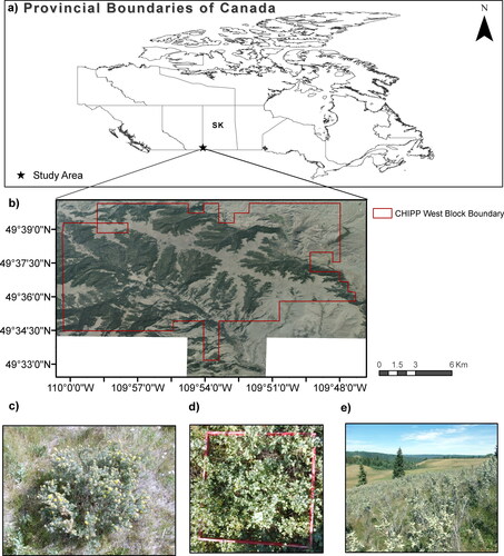
The fescue grasslands of Cypress Hills Interprovincial Park (CHIPP) in Canada (49° 40′ N, 110° 15′ W) are a mosaic of topographically heterogeneous forest and grassland that rise above the surrounding agriculture and rangelands of Saskatchewan and Alberta, Canada (Figure 1a,b). CHIPP’s grasslands are recognized for their ecological and economic significance and are undergoing shrub encroachment by native species (Widenmaier & Strong 2010; Government of Alberta 2011; Government of Saskatchewan 2021; Robinov et al. 2021). Therefore, we chose the Saskatchewan West Block portion of the park (138.19 km²) as our case study to conduct this research. The main grassland types in the study area are (1) rough fescue (Festuca campestris)-dominated grasslands present on the black and dark grey soils of the upper slopes and plateaus, covering approximately 40% of the park, and (2) mixed-grass prairie (i.e. Hesperostipa spp., Bouteloua gracillis, Koeleria macrantha, Elymus lanceolatus) established on the dark brown soils of the drier slopes and lower elevations (Sauchyn 1990; Padbury & Acton 1999; Government of Alberta 2011). For the West Block, almost all sites are on loamy black soil, whereas 25% of the area in the northeast are classified as dark brown soils (Godwin & Thorpe 1994). Two large streams found in the West Block are Battle Creek, which dissects the park and receives input from Reesor Lake, and Nine Mile (Government of Alberta 2011). The main shrub species of concern are shrubby cinquefoil (Potentilla fruticosa) (Figure 1c), western snowberry (Symphoricarpos occidentalis) (Figure 1d) and wolf willow, also known as silverberry (Elaeagnus commutata) (Figure 1e) (field observation). All three shrubs are considered native and unpalatable to livestock (Moss et al. 2008).

Figure 1. a) Cypress Hills Interprovincial Park (CHIPP) boundary of the West Block within the provincial boundaries of Saskatchewan (SK), Canada, b)) Cypress Hills Interprovincial Park (CHIPP) boundary of the West Block overlaid on the 8-bit mosaicked aerial image of 17 October 2018, c) shrubby cinquefoil (Potentilla fruticosa), d) western snowberry (Symphoricarpos occidentalis) and e) wolf willow, also known as silverberry (Elaeagnus commutata) in the West Block of Cypress Hills Interprovincial Park (August 2020, personal collection). Source of Canadian Provincial Boundaries: Statistics Canada (Open-Government License—Canada) (Statistics Canada 2020), source of aerial image and CHIPP boundary layer: Ministry of Parks, Culture, and Sports, Government of Saskatchewan.

The annual mean temperature in Cypress Hills is 3.3 °C with a maximum of 23.2 °C in July, and a minimum of −15 °C in January (Environment and Climate Change Canada 2021). Annual mean precipitation is approximately 600 mm (Environment and Climate Change Canada 2021), and 42% of all precipitation comes from snowfall.

Data acquisition

We obtained six orthorectified aerial images of the study area at 30 cm spatial resolution from the Ministry of Parks, Culture and Sports (Government of Saskatchewan, Canada). The images were acquired on 17 October 2018 between 15:30 and 18:40 with a Vexcel UltraCamXp camera that has four channels (Red, Green, Blue, and Near Infrared). All GIS layers related to topo-edaphic variables were provided by the Ministry of Parks, Culture and Sports, Saskatchewan, Canada, and the Digital Elevation Model (DEM) was obtained from the Saskatchewan Geospatial Imagery Collaborative (SGIC) (Table 1).

Table 1. Topo-edaphic variables examined in relation to shrub cover in CHIPP’s West Block.

Variable	Details	Data type	Source
Landscape unit	Combination of Rangeland Ecosite & Topography class	Categorical	2018 CHIPP Forest Inventory
Rangeland ecosite	Defined from topography, soil texture, moisture regime, salinity	Categorical
Elevation	Upland & Lowland (above and below average elevation)	Categorical	Saskatchewan Geospatial Imagery Collaborative (SGIC)
	Full range (15 m spatial resolution)	Continuous
Aspect	4 compass directions	Categorical	Derived from SGIC Digital Elevation Model (DEM)
Slope	Classes of 10% slope rise	Categorical
	Full range (15 m spatial resolution)	Continuous
Topography	Depressional, Flat, Gully, Hilly, Steep, and Undulating	Categorical	2018 CHIPP Forest Inventory
Soil Moisture Regime (SMR)	Based on moisture availability for vegetation growth (based on SK Forest Vegetation Inventory)	Categorical	2018 CHIPP Forest Inventory
Distance from watercourse lines	Euclidean distance, 15 m spatial resolution (Part of the ‘Lakes, Rivers and Glaciers in Canada-CanVec Series-Hydrographic Features’)	Continuous	Government of Canada
Distance from wetlands	Euclidean distance, 15 m spatial resolution (Digitized by Geomatics Canada)	Continuous	National Topographic Data Base
Distance from waterbodies	Euclidean distance (15 m spatial resolution)	Continuous	Ministry of Parks, Culture and Sport (Saskatchewan, Canada)

Methodology

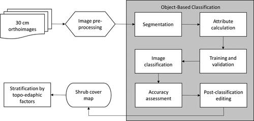
Figure 2 demonstrates the procedures we followed in this study. We first mosaicked all the images and then clipped the image to the grassland polygons based on the Forest Inventory database (2018) provided by the park. To reduce the processing time, the image was divided into four tiles following natural boundaries. All processing was conducted in PCI Geomatics Banff (2018). The object-based shrub classification mapping process included segmentation, attribute calculation, collection of training and validation data, image classification, accuracy assessment, and post-classification editing. Each are detailed below.

Figure 2. Flowchart of methods used to map shrub cover in Cypress Hills Interprovincial Park’s (CHIPP) and stratify this cover by topo-edaphic factors.

Segmentation

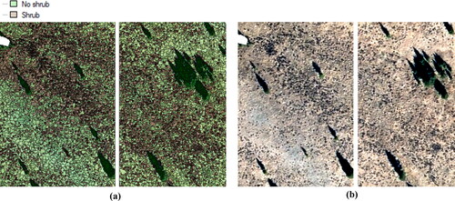
We defined the parameters of scale, shape and compactness first (Niphadkar et al. 2017). The scale parameter takes values between 0 and 100. Large scale parameters permit a high level of heterogeneity (Arasumani et al. 2021). Thus, for a given scale parameter, a heterogeneous image will yield smaller objects than a homogeneous image (Niphadkar et al. 2017). The shape parameter ranges from 0 to 0.9. Lower shape values assign more weight to spectral values and higher values indicate more importance of shape over spectral values (Arasumani et al. 2021). Compactness (ranging from 0 to 1) identifies the compressed nature of the objects, based on weak spectral contrasts, and is used to optimize objects for their compact shape (Niphadkar et al. 2017). To determine the segmentation parameters, we started with the default ones, as determined in the Object Analyst workflow of PCI Geomatics, which were Scale = 25, Shape= 0.5, and Compactness = 0.5. After a few repetitions of trial and error, and by visually looking at the resulting segmented objects, the parameters that defined the small shrubs as single objects in our study area were Scale = 5, Shape = 0.5, and Compactness = 0.5. Figure 3a shows a close up of the segmentation result in the southeast part of our study area with the derived object segments, and Figure 3b shows the respective aerial image of that location.

Figure 3. a) Detail of segmentation result in the southeast part of our study area with the derived object segments for the ‘shrub’ and ‘no shrub’ classes, and b) the respective aerial image of this location.

Attribute calculation

We calculated several attributes for each segmented object and image channel that facilitated the subsequent shrub classification (Table 2). We first calculated pure statistics for the Digital Number (DN) range of each channel. Then, we calculated the geometrical attributes of circularity, solidity and compactness, which could be higher for shrub segments compared to grass segments. Although the aerial imagery is not calibrated to reflectance (DN number), we used vegetation indices (VIs) (e.g. Normalized Difference Vegetation Index-NDVI, Soil Adjusted Vegetation Index-SAVI, and Transformed Vegetation Index-TVI) to differentiate between shrubs and background cover (grass, bare soil, etc.) based on number ratios (Hantson et al. 2012; Hellesen & Matikainen 2013; Ng et al. 2017; Niphadkar et al. 2017). Lastly, we calculated textural features in a 5 × 5 pixel window size.

Table 2. Attributes calculated for each image object (GRVI = Green-Red Vegetation Index, GI = Greenness Index, VDI = Vegetation Dryness Index, RVI = Ratio Vegetation Index, NDVI = Normalized Difference Vegetation Index, TDVI = Transformed Difference Vegetation Index, SAVI = Soil Adjusted Vegetation Index, MSAVI2= Modified Soil Adjusted Vegetation Index, GEMI = Global Environmental Monitoring Index, LAI = Leaf Area Index).

Attribute Category	Attributes	Channels used
Statistical	Min; Max; Mean; Standard Deviation	R, G, B, NIR
Geometrical	Circularity; Compactness; Solidity	/
Spectral	GRVI; GI; VDI; RVI; NDVI; TDVI; SAVI; MSAVI2; GEMI; LAI	R, G, NIR
Textural^*	Mean; Standard deviation; Entropy; Angular second moment	R, G, B, NIR

* (5 × 5 window size).

Training and validation

We collected training and validation samples through visual image interpretation of the aerial image. Each sample corresponds to a segmented object, which was collected through their selection in Object Analyst. We generated two classes; ‘Shrub’ and ‘No Shrub’ to collect presence and absence data. A total of 1200 training objects and 800 validation objects for each class were collected, resulting in a total of 2000 objects for each class. Hence, 60% was training data and 40% was validation data. This ratio was selected to ensure enough data variance is captured in the validation dataset since the ‘Shrub’ and ‘No Shrub’ classes are heterogeneous in the grassland ecosystem. Moreover, we preferred a lower percentage of training data to avoid overfitting the model that is used during image classification. The objects were randomly collected with good distribution, ensuring enough heterogeneity per class, so that they are representative.

Image classification and post-classification editing

We used the non-parametric SVM classification algorithm to train the model. This algorithm was implemented in PCI Geomatics Banff through the Object Analyst workflow, which is based on the open-source code LIBSVM (developed and described in Hsu et al. (2016)). The SVM algorithm tries to find the optimal hyperplane that separates two classes by maximizing their margin; this is realized by analysing the training samples at the edge of each class, otherwise referred to as support vectors. It applies a mathematical kernel function to map the support vectors from the training data into a higher-dimensional space (hyperplane) to separate the two classes (PCI Geomatics 2020). There are several kernels that can be used, as described in Hsu et al. (2016). The authors recommend the use of the radial-basis function (RBF) since it can include non-linear relationships between the classes and attributes used, it has less numerical difficulty compared to polynomial kernels, and can behave similar to a linear or sigmoid kernel for certain parameters. Therefore, we used the RBF kernel. There are two parameters that need to be selected to run the SVM algorithm with the RBF kernel, C and γ (see Hsu et al. (2016) for more information). We selected these parameters using a grid-search with cross-validation (i.e. different pairs of values for C and γ were used in model runs, and the one with the best cross-validation accuracy for the training samples was selected). Once we found the best parameters, we trained the model with the training set to generate the final classifier. After the final classifier was applied to the whole image, we applied post-classification editing, which dissolved neighbouring image segments of the same class into one shape, through which individual shrubs remained a single object and shrub patches became one main object.

Finally, we used an accuracy assessment to get an overview of the classification model performance. The accuracy assessment was performed at object level, during which each of the object classes in the validation dataset are compared to the equivalent object class in the classified image. If the classes are equal (or unequal) to each other, the object is considered correctly (or incorrectly) classified. The measures of assessment that we calculated include the overall accuracy, the producer’s and user’s accuracy for each class (i.e. shrub and no shrub), and the overall kappa statistic. Overall accuracy is the number of total correctly classified samples divided by the total number of samples. The producer’s accuracy is estimated for each class, and looks at the number of correctly classified samples divided by the total number of validation samples in that class; the misclassified number of samples are considered omission errors (the number of known samples that were not included in that class). The user’s accuracy is also estimated for each class, and is equal to the total number of correctly classified samples of a class divided by the actual number of samples included in that class; the misclassified number of samples are considered commission errors (samples that were not included in the correct class in the classified image). Lastly, the overall kappa statistic is used to determine if the classification is significantly better than chance (it is expressed on a scale of 0 to 1).

Stratification by topo-edaphic factors

We examined the shrub cover distribution over the available topo-edaphic variables of the study area (Table 1), which included landscape units, rangeland ecosites, topography, elevation, aspect, slope, soil moisture regime, watercourse, waterbodies, and wetlands. CHIPP’s landscape units (22 classes in total) (Figure A1) are a combination of four rangeland ecosites (Gravelly, Loam, Overflow, and Thin) (Figure A2), as defined in ‘Ecoregions and Ecosites’ of the Saskatchewan Prairie Conservation Action Plan (Thorpe 2014), and six topography classes (Depressional, Flat, Gully, Hilly, Steep, an Undulating) present in the 2018 Forest Inventory Map of the park (Figure A3). The rangeland ecosites are classified based on differences in topography, soil texture, moisture regime, and salinity (Thorpe 2014). For the categorical variables, we calculated the % shrub cover in each class of a variable by dividing the total shrub area in each class by the total area of that class. For the continuous variables, we calculated the % shrub cover in each 15 × 15 m pixel and then plotted multiple regression models against the continuous value of each 15 × 15 m pixel.

Moreover, we examined categorical and continuous variables for elevation. First, we separated the grassland region into ‘Upland’ and ‘Lowland’ based on the average elevation (Figure A4). Both classes cover about the same area of grasslands in the park (Uplands = 51.2%, Lowlands = 48.8%). Second, we used the continuous elevation range from the SGIC Digital Elevation Model (DEM) at 15 m spatial resolution. We calculated shrub cover in each 15 × 15 m pixel of the DEM and juxtaposed this cover with every unique elevation value. The aspect values were derived from the DEM and reclassified into four compass directions: Flat (−1 and −1–0), North (0–67.5 and 292.5–360), East (67.5–112.5), South (112.5–247.5), and West (247.5–292.5). Lastly, slope values, expressed in % rise, were also derived from the DEM. We examined categorical and continuous variables for slope. We separated % slope rise in the grassland regions in classes of 10%, ranging from 0 to 290%, resulting in a total of 29 classes, and we also used the continuous values of slope % rise (juxtaposed to each 15 × 15 m shrub cover pixel).

Lastly, we included four layers related to water and moisture. The first one is the Soil Moisture Regime (SMR), which represents the availability of moisture for vegetation growth (Saskatchewan Environment-Forest Service 2004) – seven classes ranging from ‘Dry’ to ‘Very Moist’ are available in the study area (Figure A5). The other three layers are related to the hydrographic features of the park, which include the watercourse lines, waterbodies, and wetland locations, which are provided in the ‘CanVec Series’ through the government of Canada (Government of Canada 2019). We examined the variation of shrub cover based on their Euclidean distance from each of these hydrographic features in a 15 m resolution raster.

Results

Shrub cover

The overall accuracy of the SVM classification for all four image tiles ranged between 92% and 95% with a lower 95% confidence interval (CI) between 89.2% and 92.7% and an upper 95% CI between 94.8% and 97.3%, while the overall Kappa statistic ranged between 0.84 and 0.9 (Table 3). The producer’s and user’s accuracy for the ‘shrub’ class ranged between 90.5% and 95%, and between 93.3% and 95%, respectively (Table 3). The producer’s and user’s accuracy for the ‘no shrub’ class ranged between 93.5% and 95%, and between 90.8% and 95%, respectively (Table 3). The total shrub cover in the grasslands of CHIPP’s West Block in Saskatchewan is 17.02 km², which represents 27.3% of the total grassland area in the park. The shrub cover map of CHIPP’s West Block is presented in Figure 4. The northwest area has the highest shrub cover (approx. 34%).

Figure 4. a) Shrub cover in Cypress Hills Interprovincial Park’s (CHIPP) West Block overlaid on the mosaicked 8-bit aerial image, b) Closer look of heavy shrub cover on northwest plateau, c) Closer look of low shrub cover in hayed area (green boundary) in the east, d) Closer look of moderate to low shrub cover in the Battle Creek area (southwest), and e) Closer look of moderate shrub cover near waterbody in the northeast of the park.

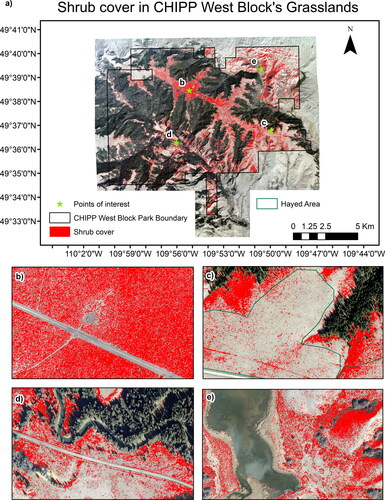
Table 3. Ranges of producer’s and user’s accuracy (PA, UA respectively) with 95% lower (L) and upper (U) confidence intervals (CI), and Kappa statistic for each class (shrub, no shrub).

Class	PA (%)	PA 95% CI-L (%)	PA 95% CI-U (%)	UA (%)	UA 95% CI-L (%)	UA 95% CI-U (%)	Kappa
Shrub	90.5–95	86.2–91.7	94.8–98.3	93.3–95	89.5–91.7	97.1–98.3	0.87–0.90
No Shrub	93.5–95	89.8–91.7	97.2–98.3	90.8–95	86.6–91.7	95–98.3	0.82–0.90
Overall classification	OA (%)	95% CI-L (%)	95% CI-U (%)	Overall Kappa
	92.0–95.0	89.2–92.7	94.8–97.3	0.84–0.90

Shrub cover by topo-edaphic factors

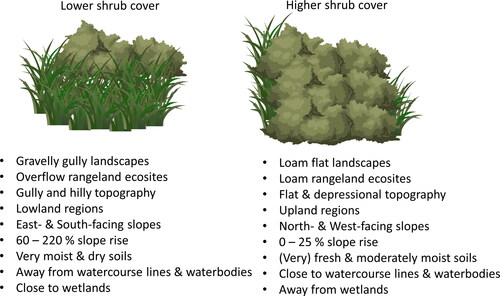
There are certain fixed topo-edaphic factors that contribute to high shrub cover in the park (Figure 5). Loam flat landscapes, flat and depressional topography, upland regions, North-facing slopes, areas with 0% to 25% slope rise, and (very) fresh and moderately moist soil moisture regimes were all connected to higher shrub cover in the park. Moreover, shrub presence was higher when closer to watercourse lines and waterbodies but lower when closer to wetlands.

Figure 5. Graphic summary of relationship between shrub cover and topo-edaphic factors in the grassland regions of the West Block in Cypress Hills Interprovincial Park (CHIPP).

Landscape unit

The highest shrub cover (39.0%) is found in ‘Thin-Depressional’ areas, followed by ‘Thin-Steep’, ‘Loam-Flat’, ‘Thin-Undulating’, and ‘Overflow-Flat’ areas (all above 33% shrub cover) (Table 4). Nevertheless, all five classes, except for ‘Loam-Flat’, represent only a small fraction (less than 5.2%) of the total grassland cover in CHIPP West Block (Table 4). The ‘Loam-Flat’ areas have the highest representation in the park (29.1%) and have high shrub cover (34.8%). Moreover, 37.7% of the total shrub cover in CHIPP’s West Block falls in Loam-Flat areas.

Table 4. Percent Landscape Unit over total grassland area, percent shrub cover by Landscape Unit, and percent shrub cover area over the total shrub cover in CHIPP West Block grasslands by Landscape Unit.

Landscape unit	% over total grassland area	% Shrub cover	% Shrub cover area over total shrub cover
Thin-depressional	0.04%	39.01%	0.05%
Thin-steep	5.17%	35.07%	6.75%
Loam-flat	29.12%	34.78%	37.70%
Thin-undulating	1.31%	33.46%	1.64%
Overflow-flat	0.95%	33.36%	1.17%
Loam-depressional	0.05%	29.73%	0.05%
Gravelly-flat	4.96%	26.93%	4.97%
Thin-flat	0.20%	26.85%	0.20%
Gravelly-hilly	2.69%	26.55%	2.66%
Overflow-depressional	0.01%	26.13%	0.01%
Loam-steep	4.32%	25.44%	4.10%
Overflow-steep	0.33%	25.43%	0.31%
Thin-gully	0.03%	23.74%	0.02%
Overflow-hilly	1.15%	23.64%	1.01%
Gravelly-steep	3.24%	22.63%	2.73%
Loam-undulating	5.23%	21.91%	4.27%
Loam-hilly	24.82%	21.90%	20.23%
Loam-gully	0.09%	21.55%	0.07%
Gravely-undulating	1.61%	21.21%	1.27%
Thin-hilly	12.75%	19.82%	9.41%
Overflow-undulating	1.87%	19.63%	1.36%
Gravelly-gully	0.08%	5.17%	0.01%

Rangeland ecosite

The ‘Loam’ ecosites have the highest shrub cover (28.0%) in the park. Shrub cover is below 25% for all other ecosites (Thin: 24.8%, Gravelly: 24.7%, Overflow: 24.1%) (Table 5). The ‘Loam’ ecosite covers 63.6% of the grasslands in the park while each of the other ecosites cover less than 20% of the grasslands (Table 5).

Table 5. Percent of each Rangeland Ecosite and Topography class over the total grassland area and percent shrub cover per Rangeland Ecosite and Topography class in the grasslands of the West Block of CHIPP.

rangeland ecosite	% Over total grassland area	% Shrub cover
Loam	63.60%	27.99%
Thin	19.49%	24.82%
Gravelly	12.61%	24.74%
Overflow	4.30%	24.10%
Topography
Hilly/Rolling	41.4%	21.7%
Flat	35.2%	33.6%
Steep	13.1%	28.6%
Undulating	10.0%	22.9%
Gully	0.2%	15.1%
Depressional	0.1%	33.1%

Topography

The ‘Hilly/Rolling’ (41.4%) and ‘Flat’ (35.2%) regions cover most of the grassland area in the park and the shrub cover is highest in the ‘Flat’ (33.6%) and ‘Depressional’ (33.1%) regions (Table 4).

Elevation

Uplands have about 5% higher shrub cover (29.3%) than lowlands (24.2%). Moreover, there is no strong linear relationship between shrub cover and elevation (r²=0.003) (Figure A6a). Nevertheless, this relationship is significant at a 90% confidence interval, with a p-value of 0.06. The elevation values follow a normal distribution, with most values in the grassland areas of the park centred around 1200 m (Figure A6b).

Aspect

Most of the aspects in CHIPP West Block are South facing (43.7%), followed by North facing slopes (34.2%). The highest shrub cover (34.6%) is found on West-looking slopes, followed by Flat (33.5%) and North (31.7%) facing slopes (Table 6). Nevertheless, 40.2% of the total shrub cover falls on North facing slopes in CHIPP West Block, and 37.2% on South facing slopes.

Table 6. Percent of each aspect class and top 5 slope classes over the total grassland area, percent shrub cover in each class, and percent shrub cover area over total shrub cover in the West Block in CHIPP.

Aspect	% Over total grassland area	% Shrub cover	% Shrub cover area over total shrub cover
South	43.86%	22.88%	37.20%
North	34.18%	31.70%	40.17%
West	10.85%	34.64%	13.93%
East	10.81%	20.78%	8.32%
Flat	0.31%	33.49%	0.38%
Top 5 Slope (% rise)	% Over total grassland area	% Shrub cover area over total shrub cover	Top 5 Slope (% rise)	% Shrub cover
0–10	71.54%	71.88%	250–260	15.61%
10–20	20.36%	20.09%	270–280	14.76%
20–30	5.92%	6.08%	0–10	14.68%
30–40	1.71%	1.64%	40–50	9.09%
40–50	0.33%	0.24%	30–40	8.70%

Slope

Slopes between 0 and 10% rise are the most common in the grassland regions of the park, representing about 71.5% (Table 6). Shrub cover is highest on steep slopes of 250–260% rise (15.6%), followed by 270–280% rise (14.8%), and 0–10% rise (14.7%) (Table 6). However, 250–260% rise and 270–280% rise represent a very small portion in the grassland regions of the park (less than 0.0004%). When looking at the continuous values of slope % rise versus shrub cover, we found that shrub cover has a polynomial relationship (5th order) with slope % rise (Figure A7). Shrub cover is around 15% at 0% slope rise, increasing up until about 25% slope (with 25% shrub cover). After that, shrub cover decreases as slope % rise increases, with a few outliers. Overall, shrub cover is highest between 5 and 45% slope rise. Its linear regression also has a significant p-value at the 99% confidence level (r²=0.33, p-value <0.001).

Soil moisture regime

‘Moderately Fresh’ SMR is the most common category in the grassland regions of the park, making up 70.7% of the study area (Table 7), with 24.6% shrub cover. Shrub cover is highest on ‘Very Fresh’ (39.6%), ‘Moderately Moist’ (38.2%), and ‘Fresh’ SMR (32.1%), and the lowest on ‘Very Moist’ (12.5%) and ‘Dry’ (14.4%) SMR (Table 7). The ‘Very Fresh’ and ‘Moderately Moist’ cover less than 5% of the grassland regions in the park, whereas the ‘Fresh’ SMR covers 22.8%.

Table 7. Percentage of soil moisture regime (SMR) classes over the total grassland area of CHIPP West Block, and shrub cover percent per SMR class in the grasslands of CHIPP West Block.

SMR	% Over total grassland area	% Shrub cover
Moderately fresh	70.71%	24.61%
Fresh	22.83%	32.13%
Very fresh	3.47%	39.59%
Dry	1.59%	14.35%
Moderately moist	0.71%	38.23%
Moist	0.62%	29.80%
Very moist	0.06%	12.51%

Distance from watercourse lines

The linear regression between shrub cover and distance from watercourse lines in the park is significant at the 99% confidence level (p-value < 0.001). However, the correlation is low (r²=0.15). Shrub cover remains between 24% and 30% as the distance from the watercourse increases, with a slight jump at around 200 m (Figure A8a); however, the number of the shrub cover samples drastically declines within the first 500 m from the watercourse lines (Figure A8b).

Distance from wetlands

There are six wetland bodies found in the northeast boundaries of the park. The linear regression between shrub cover and their distance from wetlands in the park is significant at the 99% confidence level with a moderately positive correlation (r²=0.37, p-value < 0.001) (Figure A9a). Shrub cover increases as the distance from the wetland locations increases, with a bigger jump at around 2 km. In addition, most shrub cover samples can be found up to 2.5 km from the wetlands (Figure A9b).

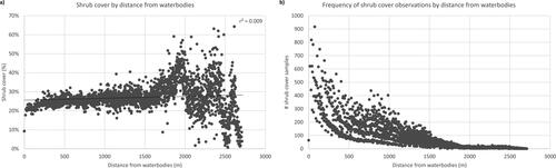
Distance from waterbodies

The linear regression between shrub cover and distance from waterbodies in the park is significant at the 99% confidence level with a very weak correlation (r²=0.01, p-value < 0.001). Shrub cover is between 20% and 30% as the distance from the waterbodies increases, with higher shrub cover ranges (above 40%) between 2 km to 2.5 km (Figure A10a); however, the number of shrub cover samples declines as we move away from the waterbodies (Figure A10b).

Discussion

We successfully mapped shrub cover in the park using an object-based approach with an overall accuracy above 92%. This result is promising, especially given the limited number of studies that have detected low stature shrubs with this approach in Northern grassland ecosystems. Dong et al. (2019) mapped low stature shrub cover in the Mongolian grasslands using higher spatial resolution imagery (2 cm) but achieved a lower overall classification accuracy (84.52% compared to ground-derived GPS points). While they also used an object-based approach, they only applied one spectral attribute feature in the classification to extract the shrub objects (i.e. the Excess Green Vegetation Index minus the Excess Red Vegetation Index). The higher accuracy in our study could be attributed to the fact that we used a total of 37 features (including statistical, spectral, geometrical, and textural attributes for each image channel). A second reason for lower accuracy in the study of Dong et al. (2019) could be related to their use of an automated shrub detection approach (unsupervised method) compared to our supervised SVM classification. Thirdly, another potential cause for lower overall classification accuracy in Dong’s study could be the use of very high spatial resolution imagery that causes issues with comparisons of GPS positioning of ground truth data (Müllerová et al. 2016). We used 30 cm resolution imagery for our object-based shrub classification and used visually estimated validation data. Our overall classification accuracy is similar to the one obtained by Levick and Rogers (2011) (i.e. 94% compared to visual estimates), who used aerial imagery of the same spatial resolution as ours and the same validation method to map shrub cover in the arid savanna ecosystem. Nevertheless, it is important to note that we did not address the potential spatial autocorrelation between the training and validation data, which can lead to an optimistic bias in the accuracy assessment results of our classification (Karasiak et al. 2022). Even though the object-based data splitting approach that we used might have removed the spatial dependence between training and validation objects (Karasiak et al. 2022), future studies should consider implementing a spatial data splitting approach to more confidently ensure that this has occurred.

As mentioned in the Introduction, Zhou et al. (2014) found that using an object-based methodology to detect shrubs was more successful than pixel-based approaches. It was argued that one reason for greater classification success is due to the fact that shrub size, shape and texture can be used during object-based classification in addition to the spectral features of shrubs. Indeed, the use of all four elements play an important role in distinguishing shrubs with an object-based classification method. Depending on the study area, shrubs can have a certain diameter size, a characteristic circular or elliptical shape (either individually or in patches), display higher roughness (texture) compared to smooth grass surface, and have spectral differences with the surrounding grasses (depending on their phenological stage) (Soubry & Guo 2022).

Current shrub cover in the park (approx. 27%), based on the 2018 aerial imagery, is above the healthy grassland standards of the region, where woody cover is naturally present at a lower abundance (<15%) (Government of Saskatchewan 2008). Since the current shrub cover in our study area is about twice as abundant as what would be expected for healthy Fescue Prairie grasslands, we conjecture that shrubs have been encroaching in the grassland regions of CHIPP’s West Block over time. However, confirmation of previous shrub cover extent from historical images of the region (30 to 40 years ago) would be necessary to validate this assumption. It is worth noting that the aerial images used in this study contained shadows, since they were obtained in the late afternoon. For this reason, we might have slightly underestimated shrub cover (areas that were missed due to shadows); however, this slight underestimation is counterbalanced with areas of slight overestimation due to possible mixture with bare ground patches and senesced grasses.

The higher shrub cover in depressional, undulating, and overflow landscape units could be related to the higher presence of moisture in the soil associated with these topographical categories (Harrington 1991; Wu & Archer 2005), thus, facilitating shrub growth (Harrington 1991). When looking at the soil moisture regimes (SMR) that had the highest shrub cover in the park, we found that the ‘Very Fresh’ SMR occurred on a variety of landscape units, while the ‘Moderately Moist’ category was predominantly found on undulating topography. The ‘Dry’ and ‘Very Moist’ SMRs had the lowest shrub cover, which can be justified by the fact that, on one hand, woody plants are less common in dry conditions (Archer et al. 2017), but, on the other hand, shrubs grow poorly in extremely wet sites due to lack of oxygen (Nuss et al. 2007). This last fact might also explain why shrub cover is lower closer to the wetland regions of the park. Moreover, although the distance from watercourse lines and waterbodies in the park did not have a strong relationship with % shrub cover, shrub cover presence was higher when closer to these two hydrological features; leading us to believe that higher plant moisture availability around water sources has some relationship with the higher presence of shrubs in the park.

In addition, moisture availability may also be favouring specific shrub species over others that do not require the same amount of moisture to reproduce. For instance, western snowberry in Saskatchewan has been found to have lower density in areas with less water availability in comparison to sites with higher water availability (Köchy & Wilson 2004). Our fieldwork in the park from the summer of 2020 showed that western snowberry was more dominant on flat and undulating topography, shrubby cinquefoil was equally dominant in various topographies, whereas wolfwillow had a higher dominance on hilly sites. Moreover, we saw a distinct spike in shrub cover at around 200 m distance from watercourse lines. Remm (2016) found that shrubby cinquefoil did not appear within a 100 m radius from water in their study area. Shrubby cinquefoil made up the majority of the shrub cover in our field-obtained samples of 2020 in the West Block of CHIPP (around 71%). Therefore, this spike at 200 m could be due to an increase of shrubby cinquefoil presence further away from the watercourse lines. A larger sample size for each shrub species is necessary to draw specific conclusions about the species’ behaviour in the park, as the previous results correspond to a total sample of 42 distributed sites.

We also saw a difference in species distribution along the elevation gradient. For example, 64% and 75% of the field sites that were dominated by western snowberry and wolfwillow, respectively, occurred in the park’s lowlands. On the other hand, 83% of the sites where shrubby cinquefoil was dominant occurred on upland regions in the park. The higher shrub cover observed on the upland regions of the park, largely described as ‘Flat regions’, might be related to the fact that there is a greater amount of precipitation of about 100 mm on the plateau in comparison to the base regions of the park (CHIPP 2020). However, these higher elevation sites might drain water faster than lower elevation sites and receive more wind, making them more sensitive to water availability. Both local topographic and hydrological features can influence water availability for woody plant growth (Lopez et al. 2019). Additionally, in Cypress Hills, for every 100 m increase in elevation, the temperature decreases about 1 °C (CHIPP 2020). The upland ‘Flat regions’, which are approximately 200 m higher than the surrounding plains, create a colder and moister climate (Hegel et al. 2009). Even though ‘Depressional’ and ‘Flat’ topography have comparable shrub cover presence (33.1% and 33.6%, respectively), the ‘Depressional’ topography regions only cover about 0.1% of the total grassland area, while ‘Flat regions’ cover 35.2%; therefore, the ‘Flat regions’ on the plateau are a higher concern for shrub cover in the park.

It was found that most of the shrub cover in the park is located on North-facing slopes, and shrub cover was high on both steep (250%–280% rise) and mid-to-low (0%–45% rise) slopes. Some studies have connected woody plant encroachment to steep slopes (Cuneo et al. 2009; Sanjuán et al. 2018), while others have found this phenomenon more prominent on mid-to-low slopes (Bragg & Hulbert 1976; Gartzia et al. 2014). Indeed, differences in woody plant distribution can be sensitive to both aspect and slope (Kennedy 1976). The cooler and moist conditions on North-facing slopes favour woody growth. However, when conditions are too shaded, North-facing slopes can limit woody growth due to temperature limitation (Soubry & Guo 2022). These results seem to differ by woody plant species. The high shrub cover on steep slopes might also be connected to the fact that cattle cannot graze on those areas (Moss et al. 2008). Future research could investigate species-specific shrub cover in the park and their relation to slope % rise.

The methodology from this research can be applied to other areas that undergo shrub encroachment. Moreover, the current results related to the topo-edaphic factors of shrub expansion in the park can be used to facilitate shrub management decisions. However, there are other factors that can be related to shrub encroachment, such as climatic and anthropogenic factors (Archer et al. 2017). To connect shrub encroachment with climatic factors, long term data are needed (at least 30 years). This is where the use of historical aerial images can be useful. In this research, shrub cover was mapped for 2018. Therefore, results from the analysis correspond to that one point in time. Future research will include historical aerial imagery, to provide insight into where shrub expansion occurred. However, we acknowledge that it can be difficult to generate consistent shrub cover maps using historical imagery with an object-based approach since there are a number of parameters that can vary in image acquisition, such as seasonality, time of day, sensor type, and calibration (Warkentin et al. 2020). Lastly, it is important to see if anthropogenic actions in the park are more significant drivers of shrub encroachment than fixed topo-edaphic factors, or if it is a combination of both. This will also be included in our future investigation. The main anthropogenic features that are found in the park include seasonal domestic grazing, road networks and hiking trails, campgrounds, and haying practices (Government of Alberta 2011).

Conclusions

We successfully mapped shrub cover in the park using object-based classification (overall accuracy > 92%). Our results indicate that shrub cover is above the healthy grassland standards within the park. We further identified topo-edaphic variables that are connected to high shrub cover in the park. Our results suggested that shrub cover was at least partially explained by moisture availability. Landscape units with topographies and soil types related to higher moisture had higher shrub cover; and, shrub presence was higher close to watercourse lines and waterbodies. Moreover, uplands and West- and North-facing slopes, which are considered to have more moisture, also had higher shrub cover. These findings are in line with the habitat preferences of the particular shrub species in the park and with results from the literature. We believe these methods can be used to successfully map shrub cover and investigate its connection to topo-edaphic factors in other northern grassland regions. Future studies should also incorporate historical shrub mapping in combination with climatic and anthropogenic factors to get a holistic understanding of the drivers of shrub encroachment in each region.

Acknowledgements

We thank the Saskatchewan Ministry of Parks, Culture and Sport for proving GIS data and aerial imagery through project number LPU-003RE-202122. We also thank the five anonymous reviewers for their useful suggestions, which helped us improve this research article.

Data availability

Data is available upon reasonable request to the Saskatchewan Ministry of Parks, Culture and Sport.

Disclosure statement

No potential conflict of interest was reported by the authors.

Additional information

Funding

This research was funded by the Ministry of Parks, Culture and Sports, Government of Saskatchewan and the article processing charges were funded by The Natural Sciences and Engineering Research Council of Canada (NSERC) under project number LPU-003RE-202122 and grant number RGPIN-201603960.

Appendix

Figure A1. Landscape units of CHIPP West Block.

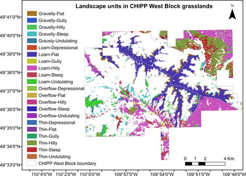
Figure A2. CHIPP West Block’s grasslands by Range Ecosite classification.

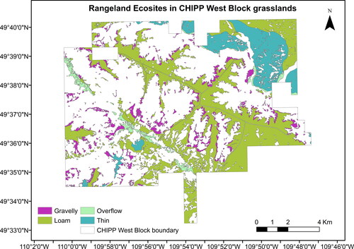
Figure A3. Topography classes in CHIPP West Block’s grasslands.

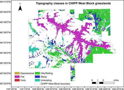
Figure A4. CHIPP West Block grassland regions by elevation class.

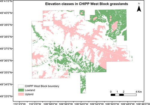
Figure A5. Soil Moisture Regimes in CHIPP West Block’s grasslands.

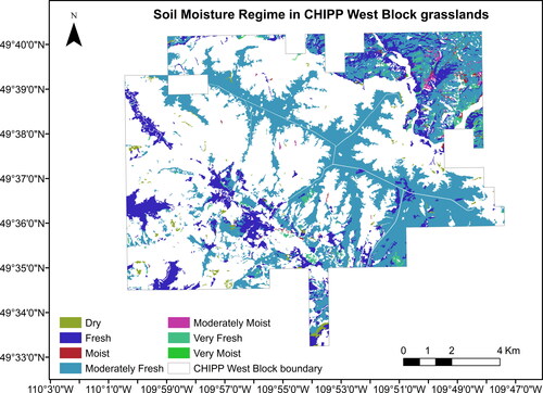
Figure A6. a) Shrub cover % per 15 x 15 m pixel by elevation value (in meters) for the grassland region of CHIPP West Block, b) Frequency of shrub cover observations per unique elevation value in the grassland areas of CHIPP West Block.

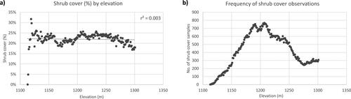
Figure A7. Percent shrub cover by slope % rise in CHIPP West Block’s grasslands.

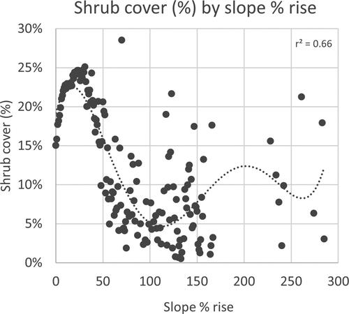
Figure A8. a) Shrub cover % per 15 x 15 m pixel versus distance (in meters) from the watercourse lines of CHIPP West Block, b) Number of shrub cover samples per distance value from the watercourse lines in the grassland areas of CHIPP West Block.

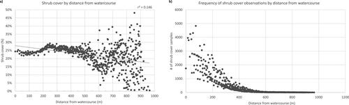
Figure A9. a) Shrub cover % per 15 x 15 m pixel versus distance (in meters) from the wetlands in CHIPP West Block, b) Number of shrub cover samples per distance value from the wetlands in the grassland areas of CHIPP West Block.

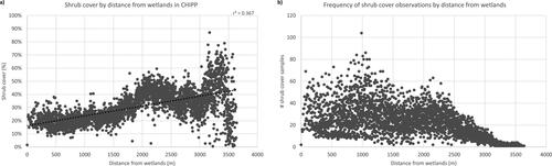
Figure A10. a) Shrub cover % per 15 x 15 m pixel versus distance (in meters) from the waterbodies in CHIPP West Block, b) Number of shrub cover samples per distance value from the waterbodies in the grassland areas of CHIPP West Block.

References

- Arasumani M, Bunyan M, Robin VV. 2021. Opportunities and challenges in using remote sensing for invasive tree species management, and in the identification of restoration sites in tropical montane grasslands. J Environ Manage. 280:111759.
- Archer SR. 2010. Rangeland conservation and shrub encroachment: new perspectives on an old problem. In du Toit JT, Kock R, Deutsch JC, editors. Wild rangelands conserv wildl while maint livest semi-arid ecosyst. 1st ed. Arizona: Blackwell Publishing; p. 53–97.
- Archer SR, Andersen EM, Predick KI, Schwinning S, Steidl RJ, Woods SR. 2017. Woody plant encroachment-causes and concequences. In Briske DD, editor. Rangel syst manag challenges. Cham (Switzerland): Springer Series on Environmental Management, Springer; p. 25–84.
- Bragg TB, Hulbert LC. 1976. Woody plant invasion of unburned kansas bluestem prairie. J Range Manag. 29(1):19–24.
- Cao X, Liu Y, Cui X, Chen J, Chen X. 2019. Mechanisms, monitoring and modeling of shrub encroachment into grassland: a review. Int J Digit Earth. 12(6):625–641.
- Caracciolo D, Istanbulluoglu E, Noto LV, Collins SL. 2016. Mechanisms of shrub encroachment into Northern Chihuahuan Desert grasslands and impacts of climate change investigated using a cellular automata model. Adv Water Resour. 91:46–62.
- CHIPP. 2020. Cypress hills interprovincial park – Park Info [Internet]. [accessed 2020 Apr 28]. http://www.cypresshills.com/visitor-information/cypress-hills-info.
- Cuneo P, Jacobson CR, Leishman MR. 2009. Landscape-scale detection and mapping of invasive African Olive (Olea europaea L. ssp. cuspidata Wall ex G. Don Ciferri) in SW Sydney, Australia using satellite remote sensing. Appl Veg Sci. 12(2):145–154.
- Dong Y, Yan H, Wang N, Huang M, Hu Y. 2019. Automatic identification of shrub-encroached grassland in the Mongolian plateau based on UAS remote sensing. Remote Sens. 11(13):1623.
- Eldridge DJ, Soliveres S, Bowker MA, Val J. 2013. Grazing dampens the positive effects of shrub encroachment on ecosystem functions in a semi-arid woodland. J Appl Ecol. 50(4):1028–1038.
- Environment and Climate Change Canada. 2021. Canadian climate normals 1981-2010 station data—Cypress Hills, Saskatchewan.
- Gartzia M, Alados CL, Pérez-Cabello F. 2014. Assessment of the effects of biophysical and anthropogenic factors on woody plant encroachment in dense and sparse mountain grasslands based on remote sensing data. Prog Phys Geogr. 38(2):201–217.
- Godwin B, Thorpe J. 1994. Grazing assessment of cypress hill provincial park. [place unknown]: Environmental Technology Division.
- González-Roglich M, Swenson JJ, Villarreal D, Jobbágy EG, Jackson RB. 2015. Woody plant-cover dynamics in argentine Savannas from the 1880s to 2000s: the interplay of encroachment and agriculture conversion at varying scales. Ecosystems. 18(3):481–492.
- Government of Alberta. 2011. Cypress hills provincial park management plan. Edmonton (AB).
- Government of Canada. 2019. Lakes, rivers and glaciers in Canada – CanVec series – Hydrographic features [Internet]. [accessed 2022 Apr 2]. https://open.canada.ca/data/en/dataset/9d96e8c9-22fe-4ad2-b5e8-94a6991b744b.
- Government of Saskatchewan. 2008. Managing Saskatchewan Rangeland. 1st ed. Bruynooghe J, Macdonald R, editors. Saskatchewan: Agriculture and Agri-Food Canada.
- Government of Saskatchewan. 2021. Ecosystem-based management plan, Cypress Hills Interprovincial Park. Regina (SK): Saskatchewan Ministry of Parks Culture and Sport.
- Gray EF, Bond WJ. 2013. Will woody plant encroachment impact the visitor experience and economy of conservation areas? Koedoe. 55(1):1–9.
- Hamada Y, Stow DA, Coulter LL, Jafolla JC, Hendricks LW. 2007. Detecting Tamarisk species (Tamarix spp.) in riparian habitats of Southern California using high spatial resolution hyperspectral imagery. Remote Sens Environ. 109(2):237–248.
- Hantson W, Kooistra L, Slim PA. 2012. Mapping invasive woody species in coastal dunes in the Netherlands: A remote sensing approach using LIDAR and high-resolution aerial photographs. Appl Veg Sci. 15(4):536–547.
- Harrington GN. 1991. Effects of soil moisture on shrub seedling survival in semi-arid grassland. Ecology. 72(3):1138–1149.
- Hegel TM, Gates CC, Eslinger D. 2009. The geography of conflict between elk and agricultural values in the Cypress Hills, Canada. J Environ Manage. 90(1):222–235.
- Hellesen T, Matikainen L. 2013. An object-based approach for mapping shrub and tree cover on grassland habitats by use of liDAR and CIR orthoimages. Remote Sens. 5(2):558–583.
- Hoff DL, Will RE, Zou CB, Weir JR, Gregory MS, Lillie ND. 2018. Estimating increased fuel loading within the Cross Timbers forest matrix of Oklahoma, USA due to an encroaching conifer, Juniperus virginiana, using leaf-off satellite imagery. For Ecol Manage. 409(October 2017):215–224.
- Hsu C-W, Chang C-C, Lin C-J. 2016. A practical guide to support vector classification. Taipei: National Taiwan University.
- Hudak AT, Wessman CA. 1998. Textural analysis of historical aerial photography to characterize woody plant encroachment in South African Savanna. Remote Sens Env. 66(3):317–330.
- Karasiak N, Dejoux JF, Monteil C, Sheeren D. 2022. Spatial dependence between training and test sets: another pitfall of classification accuracy assessment in remote sensing. Mach Learn. 111(7):2715–2740.
- Kattenborn T, Lopatin J, Förster M, Braun AC, Fassnacht FE. 2019. UAV data as alternative to field sampling to map woody invasive species based on combined Sentinel-1 and Sentinel-2 data. Remote Sens Environ. 227:61–73.
- Kennedy BA. 1976. Valley-side slopes and climate. Geomorphol Clim. 185–187.
- Knapp AK, Briggs JM, Collins SL, Archer SR, Bret-Harte MS, Ewers BE, Peters DP, Young DR, Shaver GR, Pendall E, et al. 2008. Shrub encroachment in North American grasslands: Shifts in growth form dominance rapidly alters control of ecosystem carbon inputs. Glob Chang Biol. 14(3):615–623.
- Köchy M, Wilson SD. 2004. Semiarid grassland responses to short-term variation in water availability. Plant Ecol. 174(2):197–203.
- Levick SR, Rogers KH. 2011. Context-dependent vegetation dynamics in an African savanna. Landscape Ecol. 26(4):515–528.
- Lopez EL, Kerr SA, Sauchyn DJ, Vanderwel MC. 2019. Variation in tree growth sensitivity to moisture across a water-limited forest landscape. Dendrochronologia. 54:87–96.
- Lu D, Weng Q. 2007. A survey of image classification methods and techniques for improving classification performance. Int J Remote Sens. 28(5):823–870.
- Marston CG, Aplin P, Wilkinson DM, Field R, O’Regan HJ. 2017. Scrubbing up: multi-scale investigation of woody encroachment in a Southern African savannah. Remote Sens. 9(5):419.
- Mirik M, Ansley RJ. 2012. Utility of satellite and aerial images for quantification of canopy cover and infilling rates of the invasive woody species honey mesquite (Prosopis Glandulosa) on Rangeland. Remote Sens. 4(7):1947–1962.
- Moss R, Gardiner B, Bailey A, Oliver G. 2008. A guide to integrated brush management on the Western Canadian Plains. Brandon, Canada: Manitoba Forage Council.
- Müllerová J, Brůna J, Dvořák P, Bartaloš T, Vítková M. 2016. Does the data resolution/origin matter? Satellite, airborne and UAV imagery to tackle plant invasions. Int Arch Photogramm Remote Sens Spat Inf Sci – ISPRS Arch. 41(July):903–908.
- Myers VR. 2019. What is the difference between a tree and shrub? The spruce [Internet]. [accessed 2020 Jul 8]. https://www.thespruce.com/the-difference-between-trees-and-shrubs-3269804.
- Naito AT, Cairns DM. 2011. Patterns and processes of global shrub expansion. Prog Phys Geogr. 35(4):423–442.
- Ng WT, Rima P, Einzmann K, Immitzer M, Atzberger C, Eckert S. 2017. Assessing the potential of sentinel-2 and pléiades data for the detection of prosopis and vachellia spp. In Kenya. Remote Sens. 9(1):1–29.
- Niphadkar M, Nagendra H, Tarantino C, Adamo M, Blonda P. 2017. Comparing pixel and object-based approaches to map an understorey invasive shrub in tropical mixed forests. Front Plant Sci. 8(May):1–18.
- Nuss R, Guiser S, Sellmer J. 2007. Trees, shrubs, and groundcovers tolerant of wet sites [Internet]. [accessed 2022 Apr 8]. https://extension.psu.edu/trees-shrubs-and-groundcovers-tolerant-of-wet-sites.
- O’Connor CR. 2019. Drivers, mechanisms, and thresholds of woody encroachment in mesic grasslands. Manhattan (KN): Kansas State University.
- Padbury GA, Acton DF. 1999. Wildlife-ecoregions. In Ka-iu Fung, editor. Atlas of Saskatchewan. 2nd ed. Saskatoon (SK): University of Saskatchewan; p. 160–162.
- PCI Geomatics. 2020. Support vector machine classifier [Internet]. [accessed 2020 Jul 7]. https://support.pcigeomatics.com/hc/en-us/sections/200665249-Geomatica-Training-Guides.
- Poznanovic AJ, Falkowski MJ, Maclean AL, Smith AMS, Evans JS. 2014. An accuracy assessment of tree detection algorithms in juniper woodlands. Photogramm Eng Remote Sensing. 80(7):627–637.
- Pracilio G, Smettem KRJ, Bennett D, Harper RJ, Adams ML. 2006. Site assessment of a woody crop where a shallow hardpan soil layer constrained plant growth. Plant Soil. 288(1–2):113–125. doi:10.1007/s11104-006-9098-z.
- Remm K. 2016. Selecting site characteristics at different spatial and thematic scales for shrubby cinquefoil (Potentilla fruticosa L.) distribution mapping. For Stud. 64(1):17–38.
- Robinov L, Hopkinson C, Vanderwel MC. 2021. Topographic variation in forest expansion processes across a mosaic landscape in Western Canada. Land. 10(12):1355–1318.
- Sanjuán Y, Arnáez J, Beguería S, Lana-Renault N, Lasanta T, Gómez-Villar A, Álvarez-Martínez J, Coba-Pérez P, García-Ruiz JM. 2018. Woody plant encroachment following grazing abandonment in the subalpine belt: a case study in northern Spain. Reg Environ Change. 18(4):1103–1115.
- Saskatchewan Environment-Forest Service. 2004. Saskatchewan Forest Vegetation Inventory – forest planning manual. Prince Albert (SK).
- Sauchyn DJ. 1990. A reconstruction of Holocene geomorphology and climate, western Cypress Hills, Alberta and Saskatchewan. Can J Earth Sci. 27(11):1504–1510.
- Scholtz R, Polo JA, Fuhlendorf SD, Engle DM, Weir JR. 2018. Woody plant encroachment mitigated differentially by fire and herbicide. Rangel Ecol Manag. 71(2):239–244.
- Shivakanth G, Tanwar PS. 2018. Review on conventional and advanced classification approaches in remote sensing image processing. IJCSE. 6(11):871–879.
- Soubry I, Guo X. 2022. Quantifying woody plant encroachment in grasslands: a review on remote sensing approaches. Can J Remote Sens. 48(3):1–42.
- Statistics Canada 2020. 2016 census-boundary files [Internet]. [accessed 2021 Jan 20]. https://www12.statcan.gc.ca/census-recensement/2011/geo/bound-limit/bound-limit-2016-eng.cfm.
- Swanson RE. 1994. A field guide to the trees and shrubs of the southern Appalachians. Baltimore (UK): The Johns Hopkins University Press.
- Thorpe J. 2014. Ecoregions and ecosites. Saskatchewan: Prairie Conservation Action Plan.
- Van Auken OW. 2000. Shrub invasions of North American semiarid grasslands. Annu Rev Ecol Syst. 31(1):197–215.
- Warkentin K, Stow D, Uyeda K, O’Leary J, Lambert J, Loerch A, Coulter L. 2020. Shrub fractional cover estimation and mapping of San Clemente Island shrubland based on airborne multispectral imagery and lidar data. Remote Sens. 12(21):1–20.
- Widenmaier KJ, Strong WL. 2010. Tree and forest encroachment into fescue grasslands on the Cypress Hills plateau, southeast Alberta, Canada. For Ecol Manage. 259(10):1870–1879.
- Wu XB, Archer SR. 2005. Scale-dependent influence of topography-based hydrologic features on patterns of woody plant encroachment in savanna landscapes. Landscape Ecol. 20(6):733–742.
- Zhou D, Xia Z, Dong L, Wenjiang H, Dailiang P, Linsheng H. 2014. Remote sensing identification of shrub encroachment in grassland in Inner Mongolia. Trans Chinese Soc Agric Eng. 30(11):152–158.