Using multisource satellite products to estimate forest aboveground biomass in Oita prefecture: a novel approach with improved accuracy and computational efficiency

Abstract

Accurate estimation of forest aboveground biomass (AGB) using satellite information is crucial for quantitatively evaluating forest carbon stock for climate change mitigation. However, with the emergence of an enormous number of identical data, selecting the most valuable dataset for estimation is essential to improve model efficiency and accuracy. Here, we present a novel framework using principal component analysis (PCA)-derived textures to tackle redundant variables and the integration of multisource satellite images using the random forest regression algorithm with recursive feature elimination to map the AGB of deciduous broadleaf forests in Oita prefecture, Japan. Our results highlighted that the model using PCA and derivative features had the best performance [R² = 0.69, root mean square error (RMSE) = 33.59 Mg/ha, mean absolute error = 25.01 Mg/ha, relative RMSE = 0.27]. In this case, of the 34 variables selected by RFE for the model, 19 were derived from principal components and corresponding textures, indicating a considerable improvement in using our novel framework to estimate AGB. Together, this study provides a valuable strategy for feature selection to lessen multicollinearity and redundancy.

Keywords:

• Aboveground biomass
• deciduous broadleaf forest
• random forest
• recursive feature elimination
• principal component analysis
• GLCM-Textures

1. Introduction

Forests, which cover nearly 30% of the Earth’s land surface, play a vital role in the global carbon cycle and crucially affect the Earth’s climate (Bonan 2008; Kindermann et al. 2008; Fang et al. 2014). Aboveground biomass (AGB) is a vital and popular indicator to estimate and quantify forests due to the difficulty of collecting sufficient calibrated parameters from below biomass (Amini and Sumantyo 2009). Besides, Forest AGB is also a direct source of materials and energy for human use and is recognized by the Global Climate Observing System as an essential climate variable (Bojinski et al. 2014; Rodríguez-Veiga et al. 2019). Such information is also critical to reporting for Reducing Emissions from Deforestation and Forest Degradation plus (REDD+) (Campbell 2009). The above reasons demonstrate the importance of forest AGB for its contribution to estimate both climate mitigation and carbon cycle. In Japan, forests cover nearly 25 million hectares, which accounts for 67% of the national land (Agency 2020). The deciduous broadleaf forest (DBF) in Japan is one of the most predominant forest types, sharing nearly 35% of the total forest area. Therefore, it is urgent to develop an efficient model to estimate the forest AGB on a large scale for improving forest management and responding to climate change in Japan.

Traditional approach for AGB estimation that collecting field measurement plots by human hands is recognized as the most accurate and popular method to quantify AGB (Lu 2006; Chave et al. 2014). With this method, accurate tree height and diameter measurements at breast height (DBH) are typically measured and used as variables for building allometric functions to calculate AGB calibrated by destructive samples (Chojnacky et al. 2014). However, AGB data obtained by this approach is limited by plot size, and it is impractical for a large area measurement. Currently, most of the research effort on forest estimation has demonstrated its accuracy and capacity in a large area by combining multisource remote sensing data (Lu et al. 2016). For instance, (Forkuor et al. 2020) combined Sentinel1 (S1) and Sentinel2 (S2) data and derivative data (indices, biophysical parameters) to map AGB in a dry forest area, and (Dang et al. 2019) used S2 data alone and in combination with computed S2-derived gray level co-occurrence matrix (GLCM) textures and vegetation indices to map forest AGB in Yok Don National Park, Vietnam.(Ma et al. 2017) constructed a model to estimate AGB in northeast China from PALSAR-2 data and derived topographical parameters, including elevation, slope, and aspect. ( Tariq, Shu, Li et al. 2021; Tariq et al. 2021 ) successfully analysed prescribed burning of the forest by utilizing S1 data and demonstrated remote sensing technology is beneficial for exploring forest fire. These previous studies show that optical, L-band SAR, C-band SAR, and digital elevation model (DEM) data can be used to accurately estimate forests together even if dense forests cover the study areas.

GLCM texture information from satellite images can improve the accuracy of forest AGB estimation and even decrease the effect of signal saturation in dense forest like in Japan (Haralick et al. 1973; Zhao et al. 2016; Hayashi et al. 2019). While one of the most crucial problems to utilizing GLCM textures computed from remote sensing images is the repeated information and multicollinearity because remote sensing images, especially optical multispectral images, may contain redundant information that is not needed for modelling and that may result in multicollinearity among prediction variables. Moreover, texture information is limited to be computed from each image since it will cause an unimaginable computational burden in machine learning and may cause overfitting. Instead, it is suggested that the data are first compressed and their dimensionality reduced by calculating vegetation indices (VIs) or performing principal component analysis (PCA) before texture feature extraction (Hall-Beyer 2017a). PCA of GLCM textures has been shown to be effective for image classification (Hall-Beyer 2017b), but no recent study has applied PCA before computing textures. On the other hand, PCA results in information loss and selection of the number of principal components (PCs) for interpretation is subjective. For efficient model construction, therefore, comparison of data sources and appropriate selection of features for computing texture information is very important. In our study, we first present a novel framework to lessen this problem when using machine learning approach and aimed to quantify the affection on this issue.

Random forest regression (RFR) which is an efficient machine learning algorithm based on a bagging framework has the ability to evaluate the importance of each variable (feature) in a training dataset (Breiman 2001). Although as a nonparametric model, RFR lacks interpretability, it is widely used for various forest estimation because of its excellent predictive ability (Ahmed et al. 2015; Tang et al. 2021; Wang et al. 2021; Tariq et al. 2022). However, when combing multisource remote sensing data in RFR, more variables will not necessarily produce better results and, furthermore, they are likely to increase computation time, thus making the resulting random forest (RF) model difficult to implement in practice. In addition, to develop a consistent RF model, the optimal feature subsets must be determined and a specific set of oriented variables must be provided for future study (Chan and Paelinckx 2008; Corcoran et al. 2013; Belgiu and Drăguţ 2016). Therefore, to tackle this problem we used recursive feature elimination (RFE) (Gregorutti et al. 2017) to search for the best variable group (feature subset) before hyperparameter tuning of the model, both to decrease computation time and increase the RF model score. We used RFE and texture and texture selection to reduce the number of redundant variables. By integrating these two methods, we transform the unsupervised RFE feature selection algorithm from an unsupervised to a semi-supervised algorithm.

In summary, this study had the following objectives:

1. Determine the potential of models using S1, S2, PALSAR-2, and DEM data to map DBF in Oita prefecture, Japan.

2. Compare and quantify the impact of texture information obtained from data sources with different levels of compression on forest AGB estimation accuracy.

3. Establish a cost-efficient modelling framework by specific feature selection for mapping forest AGB with high accuracy to contribute to the REDD + program.

2. Materials and methods

2.1. Study area

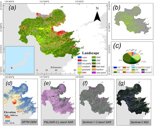
Oita prefecture located on the island of Kyushu has an area of 6,340 km² between 130°81′ −132°11′ E and 32°71′-33°74′N. It is almost entirely covered with mountains culminating up its elevation up to 1,800 m, with several mountain ranges named "Rooftop of Kyushu" to Mt. Yufu, Mt. Tsurumi, Mt. Sobo, and Mt. Katagi from north to south contributing for its various landscape and numerous species. Such kinds of the topography make it is extremely hard to obtain sufficient fields inventory plots manually for forest estimation like national forest inventory data. The forest of Oita consisted of deciduous broadleaved, evergreen needle leaved and deciduous needle leaved forest totally covering 4,484 km² land through whole range of Oita prefecture (Government and Oita Prefectural 2020). We collected the Japanese Oak (Quercus acutissima) as our collected sample plot data to develop the models because this type of species is one of the most major and predominant types DBF through our study area. High-Resolution Land Use and Land Cover (LULC) Map in Japan provided by JAXA (Figure 1a) is used to extract the targeted mapping area of DBF holding a resolution of 10 m (ver. 21.11)(JAXA 2021).

Figure 1. (a): Location of study area with land use and land cover classification. (b): Distribution pattern of DBF (c): Proportion of landscape. DBF: deciduous broadleaf forest, DNF: deciduous needleleaf forest, EBF: evergreen broadleaf forest, ENF: evergreen needleleaf forest. (d): SRTM DEM. (e): PALSAR-2 L-band SAR image displayed as RGB = HV, HH, VH in db. (f): Sentinel-1 C-band SAR image displayed as RGB = VV, VH, VV in db. (g): Sentinel-2 MSI image in true color composite (RGB = Red, Green, Blue).

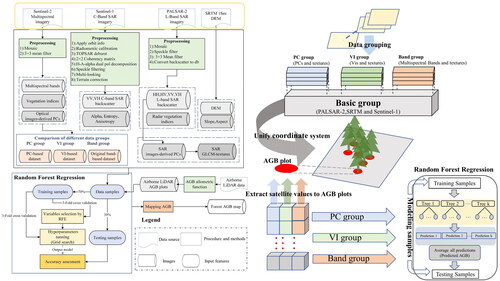
2.2. Research flow

An overview of our analytical approach is presented in Figure 2. The input data were first divided into Basic group data, consisting of data derived from PALSAR-2, SRTM, and S1 images which are not the targeted comparing images in this study. This group was first fed into the machine learning models to provide basic information for AGB estimation. This basic information, including vertical structure information from SAR data and terrestrial information from DEM data, has provided the first information for the random forest model to build preliminary model accuracy in advance. In order to provide a more objective evaluation for the performance of each group, the basic group data combined with PC, VI, or Band group data was then input into the random forest to train three corresponding models individually. We developed this procedure to objectively compare the result of the AGB estimation performance by RFR in multispectral band data with different compression levels.

Figure 2. Research flow.

2.3. Dataset

2.3.1. Airborne LiDAR data

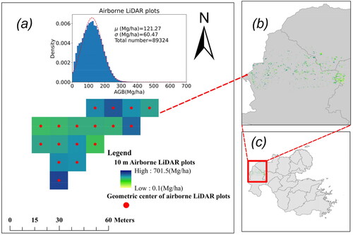
Airborne LiDAR derived data in our study served as "virtual" field data to represent a spatially “truth” data set for mapping biomass by multisource satellite images (Lu et al. 2016). This data holds a significant advantage to be used as the calibrated data to estimate AGB since it can be acquired with sufficient data sample and maintain high accuracy (Urbazaev et al. 2018). Such advantages are vital in mountainous areas where it is too hard to obtain data in the field, like in our case. PASCO Corporation (Tokyo) was commissioned by the Oita prefectural government to acquire airborne LiDAR data on Japanese oak from 5 to 17 June 2020. The data were acquired with a Leica Geosystems TerrainMapper LiDAR sensor mounted on a Cessna 208 Caravan aircraft (PASCO Co. and Ltd 2021). The sensor output was first calibrated against 11 field samples to build allometric function between forest canopy height to volume (0.02 ha, R² = 0.83). Then the LiDAR-derived Digital Canopy Height Model (DCHM) data were converted to volume data through the allometric function and aggregated into 10 m cells by calculating mean average in each 10 m cell to meet the resolution of satellite images. Finally, AGB was calculated from the volume using the biomass expansion factor, and wood density for each cell (Brown and Lugo 1984; Lehtonen et al. 2004). (1) $$\begin{array}{c}AGB=V\times WD\times \mathit{BEF}\end{array}\#$$(1) where V is stem volume (per m³), obtained from LiDAR data, and BEF (= 1.33) and WD (= 0.646 Mg/m³) are the biomass expansion factor and wood density, respectively, of Japanese oak (Ministry of the Environment 2021). A total of 89,324 AGB plots (AGB per plot: mean ± standard deviation, 121.267 ± 60.47 Mg/ha; range, 0.1–701.5 Mg/ha) in Hita city, northwest Oita prefecture, were output and used for model training in this research (Figure 3). These data are sufficient in range and amount to train a robust and accurate RF model to estimate AGB.

Figure 3. Airborne LiDAR Data. (a) example of modelling data, (b) close-up of airborne LiDAR plots, (c) Oita prefecture.

2.3.2. Remote sensing data

L-band SAR PALSAR-2 global mosaic data providing full polarization channels (HH + HV + VV + VH) for Japan was collected in 25 m resolution and prepossessed by JAXA including mosaiced, slope-corrected by AW3D30, orthorectified and converted into gamma naught (Shimada et al. 2014; JAXA 2022). We obtained C-band SAR S1 data in S1A-SLC mode, which provides dual polarization channels (VV + VH). We pre-processed it to obtain gamma naught values by applying orbit information, thermal noise removal, radiometric calibration, and terrain correction against DEM data. The features related to the H-A-alpha decomposition for S1 data were calculated via the Eigen-based way, which is available for dual-polarization mode, and then used as an additional dataset to estimate AGB (Cloude 2007).To reduce speckle noise, lessen the problem of dark spot noise and smooth the geometric error, a 5 × 5 Lee filter was applied followed by a 3 × 3 mean filter for SAR data (Lee et al. 1994; Tian et al. 2012; Peregon and Yamagata 2013). Topographical (altitude, aspect, and slope) information derived from SRTM 30-m DEM data were also used to develop the RF models in our study.

S2 optical satellite (mode L-2A) data were obtained free of charge from the European Space Agency (ESA). The data were pre-processed by the ESA by applying atmospheric correction and scene classification. The original S2 dataset comprised 13 bands with central wavelengths from 0.443 to 2.190 µm. However, bands 1, 9, and 10 were excluded because their resolution (60 m) was too coarse for high-accuracy extraction of vegetation information. To the remaining images, we also applied a 3 × 3 mean filter to reduce the effect of the spatial heterogeneity of the forest stands.

Lastly, all the satellite images were unified to the WGS_1984_UTM_Zone_52N coordinate system, mosaiced, and resampled to a resolution of 10 m by the cubic convolution method to match the resolution of the airborne LiDAR AGB data. In selecting remote sensing image scenes, we firstly considered weather conditions and then selected scenes with acquisition times as close as possible to the LiDAR data collection times to reduce the uncertainty caused by time differences. The satellite variables are summarized in Table 1.

Table 1. Summarize of satellite derived variables.

Dataset	Dates (yyyy.mm.dd)	Variables Groups	Descriptions
Sentinel-2(S2)	2020.04.06	Multispectral bands	2, 3, 4, 5, 6, 7, 8, 8A, 11, 12
		Vegetation indices	NDVI (Rouse et al. 1974), EVI (Huete et al. 2002), GARI (Gitelson et al. 1996), GCI (Gitelson et al. 2003), GDVI (Sripada 2005), GNDVI (Gitelson and Merzlyak 1998), GRVI (Sripada et al. 2006), SAVI (Huete 1988), SR (Birth and McVey 1968) and DVI (Tucker 1979)
		PCA bands	Multispectral bands derived PCA bands
		Relative Textures from multispectral bands, VIs, and PCs	Contrast, Dissimilarity, Homogeneity, Second Moment, Energy, Max Probability, Entropy, Mean, Variance and Correlation
Sentinel-1(S1)	2020.06.10	C-Band Polarization channels	VV, VH
		Polarization decomposition	Entropy, Anisotropy, Alpha
PALSAR-2	2020.08.01,2020.08.15, 2020.09.03,2020.09.17,	L-Band Polarization channels	HH, HV, VV, VH
		Radar indices	I1 (Kim et al. 2011), I2 (Huggannavar and Shetty 2020), I3 (Huggannavar and Shetty 2020)
		PCA bands and relative textures	L-Band Polarization channels derived PCA bands and its relative textures
SRTM		Topographic parameters	Elevation, Slope, Aspect

2.4. GLCM texture

In our study, we focus on the S2 data for comparison. Compared with other data, optical data holding more bands inevitably produces more redundant information, leading to severe multicollinearity in the model. So that comparison of textures derived from different sources would be as objective as possible, we sorted VIs and original bands according to their correlation with AGB sampling points before extracting texture information. We then selected them according to higher Pearson correlation coefficients, and we selected from the PCA results the number of PCs that contributed significantly to the data variance for further textures computation. We calculated 10 texture statistics for each of the three data groups: contrast (CON), dissimilarity (DIS), homogeneity (HO), second moment (SM), energy (EN), maximum probability (MAX), entropy (ENT), GLCM mean (ME), GLCM variance (VA), and GLCM correlation (COR). For this calculation, we used a window size of 5×5 pixels and a displacement of 1, 64 quantization levels, and the average of four directions (0°, 45°, 90°, and 135°) for the selected original band and VI variables. We also computed the GLCM textures for PALSAR2-derived PCs, and this is because numerous studies have proved that textures computed from L-band SAR data are advantageous in forest AGB estimation. However, the fully polarized channel will bring redundant information, so we used the PCA method for the L-band data.

2.5. Random forest regression with recursive feature elimination

The random forest regression model is optimized by feature selection and hyperparameter tuning, respectively, on four data sets as training sets, including the original bands group, VIs group, PCAs group, and all data to train models (Table 2). RFE works by searching for a subset of features by starting with all features in the training dataset and successfully removing features with a negative influence on the score, which is achieved by fitting the RFR used in the core of the model. Then RFE rank features by importance, discarding the least important features and re-fitting the model. Then the hyperparameters are optimized by grid search which exhaustively considers all hyperparameter combinations. We selected the root mean square error (RMSE) as the loss function to evaluate the performance of tunning result because it is directly related to the difference between predicted and measured values.

Table 2. Summarize of regression models.

RF-based model	Description	Total number of input features
PCA-model	Basic data, 3 PCs, and 30 relative textures.	70
VI-model	Basic data, 10 VIs, and 30 related textures.	77
Band-model	Basic data, 10 original bands, and 30 related textures.	77
All data	Basic data, 3 PCs, 10 VIs, and, 10 original bands, 90 related textures.	150

The data samples were randomly divided into training and testing data with proportions of 70:30. 3-fold cross-validation was applied to the training data for processing feature selection and hyperparameter tuning. The mean average cross-validation result was used to evaluate the output of each procedure. Finally, the testing data were used to evaluate the performance of each developed model. We calculated and compared four error statistics for model performance to select the final model: coefficient of determination (R²), RMSE, mean absolute error (MAE), and relative RMSE (rRMSE). (2) $$\begin{array}{c}{R}^2=1-\frac{\sum _{i=1}^N{\left(Y_i-Y_i^{\prime }\right)}^2}{\sum _{i=1}^N{\left(Y_i-\overline{Y}\right)}^2}\end{array}\#$$(2) (3) $$\begin{array}{c}R\mathit{MSE}=\sqrt{\frac{1}{N}{\left(Y_i-Y_i^{\prime }\right)}^2}\end{array}\#$$(3) (4) $$\begin{array}{c}MAE=\frac{1}{N}\sum _{i=1}^N\sqrt{\left|Y_i-Y_i^{\prime }\right|}\end{array}\#$$(4) (5) $$\begin{array}{c}r\mathit{RMSE}=\frac{\mathit{RMSE}}{\overline{Y}}\end{array}\#$$(5) where N is the number of observed values, $Y_{i\mathrm{ }}$ is the observed AGB value for observation i, $Y_i^{\prime }$ is the predicted AGB value, and $\overline{Y}$ is the mean of the observed AGB values. Lower RMSE, MAE, rRMSE and higher R2 indicate better performance for models.

3. Result

3.1. Determination of the PCs, VIs, and original bands to be used for texture computation

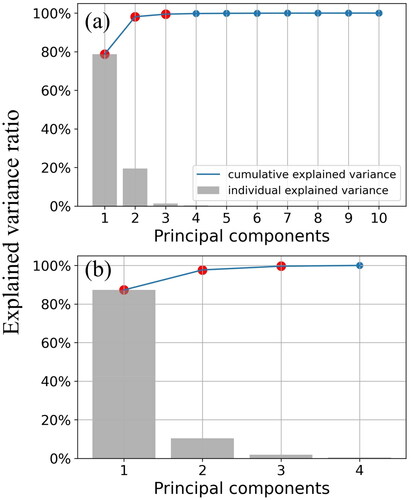
For the S2 data, the first three PCs, which accounted for 99.4% of the total variance, were used in subsequent calculations, including texture computations (Figure 4a). Regarding of PALSAR-2 data, the first two PCs, which accounted for 97.7% of the total variance, were used (Figure 4b). For comparison with the PCA results, correlations were calculated of AGB with the VIs and the original bands were calculated separately, and the three VIs and the original bands with the highest Pearson correlation coefficients were determined and their textures computed.

Figure 4. Result of PCA, the selected bands are pointed in red. (a): Sentinel-2 Multispectral Bands. (b): PALSAR-2 Polarized Channels.

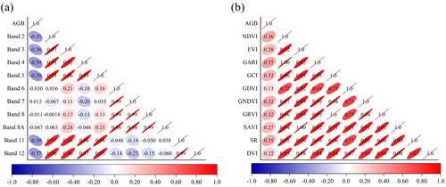
Among the original bands, bands 2, 3, 4, and 5 form one cluster, and bands 6, 7, 8, and 8a form another. A third cluster consists of bands 11 and 12. However, the correlations between AGB and bands 6, 7, 8, and 8 A are relatively weak, so the bands in this cluster were not used to compute textures. Finally, we computed texture features for bands 4, 5, and 11, the three bands with the strongest correlations, for input into the Band model (Figure 5a). NDVI, SR, and GARI were the three VIs with the strongest correlations with AGB were used to compute textures for input into the VI model (Figure 5b).

Figure 5. Coefficient matrix between AGB and Variables. (a) Bands (b) VIs.

3.2. Development of the RF models

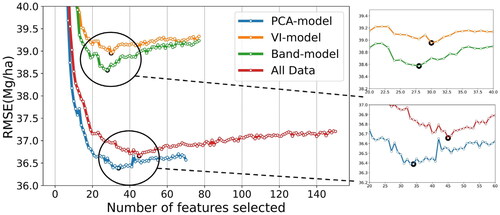
To develop an RF model, the best feature subset for prediction is first selected by RFE and then hyperparameters are adjusted. All hyperparameters are set to the default values for the RFE procedure. The RFE results for each model (Figure 6) show that the PCA model showed the best performance (RMSE = 36.39 Mg/ha) when 34 features remained, followed by All data when 45 features remained. By comparison, the VI and Band models performed poorly. Even though the PCA model features group contains a subset of all data, the addition of more variables does not necessarily result in higher RFR scores. In fact, the All-data model scores were lower than the PCA model scores. We attribute this result to the randomness in the RFR algorithm. In the process of building a basic tree, samples are randomly selected, features are randomly selected, and a subset containing k attributes from all features is randomly selected (Breiman 2001). Plus, the use of more variables with the same information but accompanied by more noise may result in lower scores because of overfitting during model training.

Figure 6. Result of RFE, the best result case of each model is indicated by black node.

Three hyperparameters were selected to be optimized by grid search: n_estimators range from 100 to 1000 with interval of 100, min_samples_leaf range from 1 to 3 and max_features which refers to number of variables fed to each predictor tree conclude three values of all observation: log₂(M), sqrt(M) and auto which equals to M. Where M is the number of observations.

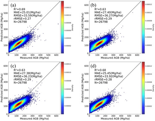
Each developed model is evaluated by testing data (Figure 7). Comparison of the predicted and measured datasets showed that among the four models, the performance of the PCA model was the best (R² = 0.69, MAE = 25.01 Mg/ha, RMSE = 33.59 Mg/ha, rRMSE = 0.27). This result indicates that, for a large dataset, the PCA model estimated AGB with high accuracy and with good stability. Although the observed AGB of some samples was under- or overestimated by the predicted AGB, these samples had little effect on the overall result. Underestimation of high AGB values is caused by the effects of the tree model and saturation, because the backscatter data cease to vary with AGB at the higher range of AGB values (Imhoff 1995; Yu and Saatchi 2016; Li et al. 2022). Overestimation of low AGB values and underestimation of high AGB values are likely a result of the way that regression trees are constructed by the RFR algorithm (Mutanga et al. 2012). Despite these limitations, our regression results show that RF models perform very well for observed AGB values within the most likely range.

Figure 7. Observed and predicted AGBs for testing samples: (a) PCA-model, (b) VI-model, (c) Band-model, (d) All data; The 1:1 line is marked by the dashed black lines.

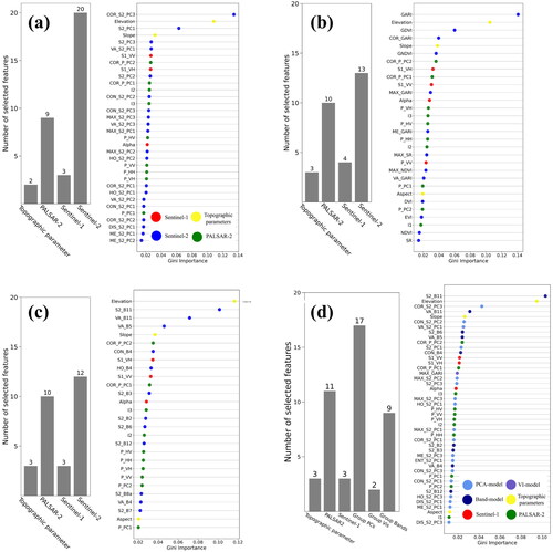
The Gini importance of the selected variables in the final RF model was also evaluated and output the ranking of features importance. The Gini importance of a RF is computed by first calculating the mean squared errors of the parent node and the left and right child nodes of the RF tree; next, optimal split selection is performed, and finally the importance of each feature in all nodes is normalized and output (Figure 8). We visualized and compared the rankings in two dimensions: According to (1) the feature importance in each of the three models (PCA, VI, and Band models), and (2) the feature importance in All data. Notably, in the best performing PCA model, the texture feature information derived from the PCs contributes significantly to the model (Figure 8a). Of the 34 selected variables in the PCA model, 20 are PCs derived from S2 data or texture information computed from the PCs. In contrast, in the VI model, 13 of 30 selected variables are VIs derived from S2 data or textures computed from the VIs, and in the Band model, 12 of 28 selected variables are original S2 bands or textures derived from those bands (Figure 8b and c). Thus, compared to the VI and Band models, the PCA model had the highest proportion of S2 data (more than 50% of all input features with the highest Gini importance scores). Because the basic data were the same in every model, the proportion of S2 features can be used to examine the influence of features with different compression levels on the RF model. In the case of All data, 23 of 45 selected variables were textures computed from PCs, VIs, or the original bands (Figure 8d). Among these 23 textures, 18 were computed from PCs. Thus, in this model, like the PCA model, textures derived from PCs account for a considerable proportion of the feature pool, demonstrating their crucial contribution to model performance. These results indicate that PC textures have enormous potential and ability for AGB estimation. In addition to S2 data, the topographic features elevation and slope data were important features in each model, whereas the numbers of PALSAR-2 and S1-related features were stable in each model with only small fluctuations in expected importance.

Figure 8. Variables listed in order of importance based on Gini importance: (a) PCA-model, (b): VI-model, (c): Band-model, (d): All data; abbreviation: S2: Sentinel-2, S1: Sentinel-1, P: PALSAR-2, others in Table 1.

3.3. Spatial distribution of AGB in Oita

The AGB of DBF in study area was generated in 10 m resolution using PCA model with selected 34 variables (Figure 9). The average and standard deviation of AGB over study area is 128.84 and 37.24 Mg/ha, respectively. AGB ranges from 32.69 to 437.72 Mg/ha, with the total amount of 14,507,596.8 Mg.

Figure 9. (a) Estimated wall-to-wall AGB of DBF in Oita prefecture, Japan. (b) Comparison of total DBF aboveground biomass (AGB) between statistical data in the Japanese forest register and the satellite-based model in city level. (c) First group. (d) Second group. Each data point represents the cumulative AGB at each of 18 cities (villages, towns, and cities) in Oita prefecture. $y^{\frac{1}{4}}\mathrm{x}$ is masked in red dotted line. 95% Confidence Interval is drawn in blue area.

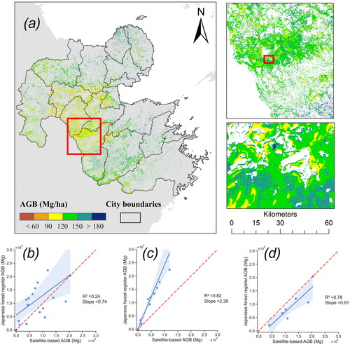
The satellite-based map was aggregated for each city and output the corresponding total AGB. We compared the result with Japanese forest registered data published by the Japanese government. It is fascinating in our result that the results of the comparison are displayed as two groups (Figure 10b–d). The first group reflects the satellite-based model with obvious lower AGB showing that points located in the above area of y = x. The second group demonstrates the results from two different sources is very close, showing a nearly parallel fitting line with y = x. We consider two dimensions that result in this difference. First, the forest register data used empirical values based on forest species and ages, first developed in the 1950s and 1960s. The non-updated data with a long gap led to significant inaccuracy(Institute 2004; Matsushita and Yoshida 1998). In addition, the saturation phenomenon underestimates forest AGB in dense forest areas like the cities that belong to the second group.

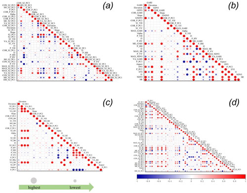
Figure 10. Correlation coefficient matrix between selected features: (a) PCA-model (b) VI-model, (c) Band-model, and (d) All data.

4. Discussion

4.1. Uncertainty and limitation on integrating multisource remote sensing data

Various types of satellite images provide copious remote sensing data for estimating AGB, and the remarkable results obtained by their utilization demonstrate the great potential of integrating multisource remote sensing data. Multisource remote sensing data can provide different types of information related to AGB that can be used to map forest AGB with high accuracy (Zhang et al. 2019). Moreover, the incorporation of multisource remote sensing data into a model can reduce the impact of data saturation (Ghosh and Behera 2018). Because of these advantages, the use of methods that integrate multisource remote sensing data improves the accuracy of forest AGB estimates.

Nevertheless, AGB estimation with multisource remote sensing data has some limitations. The toughest problem to be solved is the mismatch of time resolution between remote sensing data sources and ground-collected data. Incorporating more remote sensing data inevitably increases the likelihood of a mismatch, which may be as much as several months, between satellite data acquisition and ground data collection times. Because optical satellite images are likely to be affected by cloud cover, ways to obtain cloud-free optical satellite scenes as close as possible in time to the collection time of ground data should be investigated in future research. Furthermore, different from S1 and L-band SAR data, PALSAR-2 data are released annually as global mosaic images, where each image is a mosaic of many smaller images with different acquisition times. Thus, the collection time for a specific region within a year is fixed and may not be uniform.

4.2. Limitation of RFE in forest AGB estimation

Essentially, feature selection identifies a subset of effective variables for improved prediction by discarding insignificant variables (Jaiswal and Samikannu 2017). RFE can exclude variables that negatively affect performance, especially when there are many input variables (Mutanga et al. 2012; Pullanagari et al. 2018; Dang et al. 2019) . Our finding that the accuracy of the outcome when all data are input into the RF is a little lower than that of the PCA model obtained after RFE is also intriguing. Unlike using all data to feed into RF, the PCA model does not use the original bands and vegetation indices and their derived texture information. We consider that the performance of the PCA model was better than the other models in our study is because of redundant variables, some with noise and overlay information, are input into the RF model by All data, so that the model includes homogeneous information and noisy data. To evaluate this, we computed the mean average of variance inflation factor (VIF) in each group to detect the level of multicollinearity (Table 3). Commonly, the higher VIF indicates the higher multicollinearity effect in the regression model. It is obviously to discover that PCA-model combine with the RFE indeed significantly decrease the multicollinearity effect.

Table 3. Variance inflation factor in each group.

RF-based model	VIF
PCA-model	1126
VI-model	13247214379
Band-model	14191201649
All data	8832761381

According to (Darst et al. 2018), RF with RFE is not appropriate when many features in variable groups are highly correlated. Therefore, we recommend a new procedure for handling many features when using the RF model to estimate AGB. Instead of inputting all the variables into an RF–RFE framework, we propose that PCA should first be applied to reduce similar information contained in the predicting variables. This framework requires more experimental validation because RF models, as nonparametric models, may be represented differently in different situations. The use of PCA can also improve the interpretability of the model by reducing interpretation difficulty due to the black box nature of a nonparametric model. However, even after dimensionality reduction, multicollinearity among the variables was still present in the models, though it did not decrease the model scores (Figure 9). As a result of the bootstrap sampling (dataset sampling) and feature sampling in RFR, different feature sets are used by different models, and each model uses a different set of data points; therefore, the RF model may be unaffected by multicollinearity. To understand this phenomenon, which increases the uninterpretability of the RF model, more research is required.

4.3. Trade-off between number of PCs and model performance

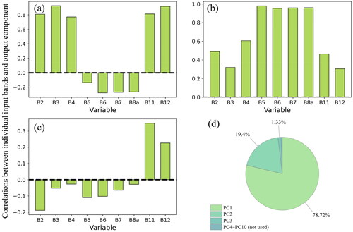
We applied PCA to extract PCs and their corresponding textures only to S2 and PALSAR-2 data, but some studies have shown that textures derived from single bands of S2 data, tomographic SAR data, and C-band SAR data all have a strong ability to estimate AGB (Misra and Balaji 2017; Liao et al. 2020; Li et al. 2021). In addition, the window size used for computation of GLCM textures can also cause AGB estimation differences (Dang et al. 2019). These additional potential variables have value and should be utilized by models. However, as more different types of remote sensing data sources emerge, the calculation of these features will greatly increase the necessary model calculations and add to the difficulty of performing large-scale AGB inversion. A possible approach to the utilization of these variable s is to apply PCA repeatedly to reduce the dimensionality of the data before texture extraction, as in our study, and to choose features computed with different methods or window sizes (Hall-Beyer 2017b). However, in PCA, selection of the number of principal components is subjective. In our PCA of S2 data, PC3 accounted for only 1.33% of the total variance, but the textures derived from PC3 also contributed to the models and were included in the subset of selected features (Figure 8); thus, even a PC with a low contribution to the variance of the whole dataset can contribute to the AGB estimation (Figure 11). In addition, PCA is data-based, which means that a different dataset would yield different results with different outcomes. Therefore, there is no single best method for determining the number of PCs that should be selected. More research is required to improve and streamline the PC selection process and still obtain high-precision estimation results.

Figure 11. Correlations between individual input bands and output component, (a) PC1 78.2% of dataset variance; (b) PC2 19.4% of dataset variance; (c) PC3, 1.33% of dataset variance; (d) Summarize of PCA proportion.

5. Conclusion

Estimating forest AGB through remote sensing data is significant for measuring climate change, especially for a large area. Integrating multisource remote sensing data can improve the estimation model’s accuracy and alleviate the saturation phenomenon. Nevertheless, integrating numerous remote sensing data always increases the redundancy of the model due to multicollinearity among the variables. Most studies have developed the model without data selection, leading to severe multicollinearity and reducing the model’s robustness. Here, we alleviate the problems through a novel framework for feature selection by integrating multisource remote sensing data and related features.

We develop a cost-efficient and elegant framework for AGB estimation using RF algorithm: (1) utilizing PCA to extract textures information instead of extracting textures from original bands or VIs. (2) Selecting features with the RFE method to reduce the time cost for modelling and improve the scores of models by finding the best performance subset from all data. Our result demonstrates that this novel framework is quite suitable for feature selection in RF utilizing various types of satellite variables, especially now that ongoing studies prove that various kinds of satellite data have great potential for AGB estimation. Furthermore, on the part of forest management for DBF forests and the maintenance of ecological security in this species, we provide a foundation for an extensive monitoring area. In the future, our work will focus on interpreting feature importance to reduce the hard-interpretability in a non-parametric model, especially for the RF model.

Data and code availability

The data and code that support the findings of this study are available from the corresponding author, [email protected], upon reasonable request.

Acknowledgments

We gratefully thanks Dr. Mryka Hall-Beyer for her advice.

Disclosure statement

No potential conflict of interest was reported by the authors.

Additional information

Funding

This study was supported by JAXA Research Announcement on the Earth Observations (No. ER2A2N208, ER3A2N122). The airborne LiDAR data and administrative data were provided by the Oita Prefectural Government (approval No. RINKAN-710 dated June 9, 2021, and No. 3-60 dated December 3, 2021). This research was funded by the Telecommunications Advancement Foundation.

Appendix

Table Appendix 1. Vegetation indices calculated from Sentinel-2 and PALSAR-2 used in this study.

Source	Indices	Equations
S2
	NDVI	$\frac{(\mathit{NIR}-\mathit{Re}d)}{(\mathit{NIR}+\mathit{Re}d)}$
	EVI	$\frac{2.5\mathrm{*}(\mathit{NIR}-\mathit{Re}d)}{(\mathit{NIR}+6\mathrm{*}\mathit{Re}d-7.5\mathrm{*}\mathit{Blue}+1)}$
	GARI	$\frac{\mathit{NIR}-[\mathit{Green}-1.7\mathrm{*}(\mathit{Blue}-\mathit{Re}d)]}{\mathit{NIR}+[\mathit{Green}-1.7\mathrm{*}(\mathit{Blue}-\mathit{Re}d)]}$
	GDVI	$\mathit{NIR}-\mathit{Green}$
	GNDVI	$\frac{(\mathit{NIR}-\mathit{Green})}{(\mathit{NIR}+\mathit{Green})}$
	GRVI	$\frac{\mathit{NIR}}{\mathit{Green}}$
	SAVI	$\frac{1.5\mathrm{*}(\mathit{NIR}-\mathit{Re}d)}{(\mathit{NIR}+\mathit{Re}d+0.5)}$
	SR	$\frac{\mathit{NIR}}{\mathit{Re}d}$
	DVI	$\mathit{NIR}-\mathit{Re}d$
PALSAR-2
	I1	$HH-\mathrm{HV}$
	I2	$HH+\mathrm{HV}$
	I3	$(HV-HH)/(HH+\mathrm{HV})$

References

- Agency JF. 2020. Annual Report on Forest and Forestry in Japan. In 15. Ministry of Agriculture, Forestry and Fisheries, Japan.
- Ahmed OS, Franklin SE, Wulder MA, White JC. 2015. Characterizing stand-level forest canopy cover and height using Landsat time series, samples of airborne LiDAR, and the Random Forest algorithm. ISPRS J Photogrammetr Remote Sens. 101:89–101.
- Amini J, Sumantyo JTS. 2009. Employing a method on SAR and optical images for forest biomass estimation. IEEE Trans Geosci Remote Sens. 47(12):4020–4026.
- Belgiu M, Drăguţ L. 2016. Random forest in remote sensing: A review of applications and future directions. ISPRS J Photogrammetr Remote Sens. 114:24–31.
- Birth GS, McVey GR. 1968. Measuring the color of growing turf with a reflectance spectrophotometer 1. Agronomy J. 60(6):640–643.
- Bojinski S, Verstraete M, Peterson TC, Richter C, Simmons A, Zemp M. 2014. The concept of essential climate variables in support of climate research, applications, and policy. Bull Am Meteorol Soc. 95(9):1431–1443.
- Bonan GB. 2008. Forests and climate change: forcings, feedbacks, and the climate benefits of forests. Science. 320(5882):1444–1449.
- Breiman L. 2001. Random forests. Machine Learning. 45(1):5–32.
- Brown S, Lugo AE. 1984. Biomass of tropical forests: a new estimate based on forest volumes. Science. 223(4642):1290–1293.
- Campbell BM. 2009. Beyond Copenhagen: REDD+, agriculture, adaptation strategies and poverty. Global Environmental Chang. 19(4):397–9.
- Chan JC-W, Paelinckx D. 2008. Evaluation of Random Forest and Adaboost tree-based ensemble classification and spectral band selection for ecotope mapping using airborne hyperspectral imagery. Remote Sens Environ. 112(6):2999–3011.
- Chave J, Réjou-Méchain M, Búrquez A, Chidumayo E, Colgan MS, Delitti WBC, Duque A, Eid T, Fearnside PM, Goodman RC, et al. 2014. Improved allometric models to estimate the aboveground biomass of tropical trees. Glob Chang Biol. 20(10):3177–3190.
- Chojnacky DC, Heath LS, Jenkins JC. 2014. Updated generalized biomass equations for North American tree species. Forestry. 87(1):129–151.
- Cloude S. 2007. The dual polarization entropy/alpha decomposition: A PALSAR case study. Sci Appl SAR Polarimetry and Polarimetric Interferometry. 644:2.
- Corcoran JM, Knight JF, Gallant AL. 2013. Influence of multi-source and multi-temporal remotely sensed and ancillary data on the accuracy of random forest classification of wetlands in Northern Minnesota. Remote Sens. 5(7):3212–3238.
- Dang ATN, Nandy S, Srinet R, Luong NV, Ghosh S, Senthil Kumar A. 2019. Forest aboveground biomass estimation using machine learning regression algorithm in Yok Don National Park, Vietnam. Ecol Inform. 50:24–32.
- Darst BF, Malecki KC, Engelman CD. 2018. Using recursive feature elimination in random forest to account for correlated variables in high dimensional data. BMC Genet. 19(Suppl 1):65.
- Fang J, Guo Z, Hu H, Kato T, Muraoka H, Son Y. 2014. Forest biomass carbon sinks in East Asia, with special reference to the relative contributions of forest expansion and forest growth. Glob Chang Biol. 20(6):2019–2030.
- Forkuor G, Benewinde Zoungrana J-B, Dimobe K, Ouattara B, Vadrevu KP, Tondoh JE. 2020. Above-ground biomass mapping in West African dryland forest using Sentinel-1 and 2 datasets - A case study. Remote Sens Environ. 236:111496.
- Ghosh SM, Behera MD. 2018. Aboveground biomass estimation using multi-sensor data synergy and machine learning algorithms in a dense tropical forest. Appl Geogr. 96:29–40.
- Gitelson AA, Gritz Y, Merzlyak MN. 2003. Relationships between leaf chlorophyll content and spectral reflectance and algorithms for non-destructive chlorophyll assessment in higher plant leaves. J Plant Physiol. 160(3):271–282.
- Gitelson AA, Kaufman YJ, Merzlyak MN. 1996. Use of a green channel in remote sensing of global vegetation from EOS-MODIS. Remote Sens Environ. 58(3):289–298.
- Gitelson AA, Merzlyak MN. 1998. Remote sensing of chlorophyll concentration in higher plant leaves. Adv Space Res. 22(5):689–692.
- Government, Oita Prefectural. 2020. Oita prefecture forestry figures. In: Oita Prefectural Government.
- Gregorutti B, Michel B, Saint-Pierre P. 2017. Correlation and variable importance in random forests. Stat Comput. 27(3):659–678.
- Hall-Beyer M. 2017a. "GLCM texture: A tutorial v. 3.0 March 2017."
- Hall-Beyer M. 2017b. Practical guidelines for choosing GLCM textures to use in landscape classification tasks over a range of moderate spatial scales. Int J Remote Sens. 38(5):1312–1338.
- Haralick RM, Shanmugam K, Dinstein IH. 1973. Textural features for image classification. IEEE Trans Syst, Man, Cybern. SMC-3(6):610–621.
- Hayashi M, Motohka T, Sawada Y. 2019. Aboveground biomass mapping using ALOS-2/PALSAR-2 time-series images for Borneo’s forest. IEEE J Sel Top Appl Earth Observations Remote Sens. 12(12):5167–5177.
- Huete AR. 1988. A soil-adjusted vegetation index (SAVI). Remote Sens Environ. 25(3):295–309.
- Huete A, Didan K, Miura T, Rodriguez EP, Gao X, Ferreira LG. 2002. Overview of the radiometric and biophysical performance of the MODIS vegetation indices. Remote Sens Environ. 83(1-2):195–213.
- Huggannavar V, Shetty A. 2020. Biomass estimation using synergy of ALOS-PALSAR and landsat data in tropical forests of Brazil. Applications of Geomatics in Civil Engineering. Singapore: Springer; p. 593–603.
- Imhoff ML. 1995. Radar backscatter and biomass saturation: Ramifications for global biomass inventory. IEEE Trans Geosci Remote Sensing. 33(2):511–518.
- Institute, Forestry and Forest Products Research. 2004. "Report on program for emergent development of forest carbon stocks dataset: fiscal year 2003." In: Forestry and Forest Products Research Institute.
- Jaiswal JK, Samikannu R. 2017. Application of random forest algorithm on feature subset selection and classification and regression. Paper presented at the 2017 world congress on computing and communication technologies (WCCCT).
- JAXA. 2021. High-resolution land cover classification maps (HRLULC). edited by JAXA.
- JAXA. 2022. Global 25 m Resolution PALSAR-2 Mosaic (Ver.2.1.1), 5.
- Kim Y, Jackson T, Bindlish R, Lee H, Hong S. 2011. Radar vegetation index for estimating the vegetation water content of rice and soybean. IEEE Geosci Remote Sens Lett. 9(4):564–568.
- Kindermann G, McCallum I, Fritz S, Obersteiner M. 2008. A global forest growing stock, biomass and carbon map based on FAO statistics. Silva Fenn. 42(3):387–396.
- Lee JS, Jurkevich L, Dewaele P, Wambacq P, Oosterlinck A. 1994. Speckle filtering of synthetic aperture radar images: A review. Remote Sens Rev. 8(4):313–340.
- Lehtonen A, Mäkipää R, Heikkinen J, Sievänen R, Liski J. 2004. Biomass expansion factors (BEFs) for Scots pine, Norway spruce and birch according to stand age for boreal forests. Forest Ecol Manage. 188(1–3):211–224.
- Liao Z, He B, Quan X. 2020. Potential of texture from SAR tomographic images for forest aboveground biomass estimation. Int J Appl Earth Observ Geoinform. 88:102049.
- Li H, Kato T, Hayashi M, Wu L. 2022. Estimation of forest aboveground biomass of two major conifers in Ibaraki Prefecture, Japan, from PALSAR-2 and sentinel-2 data. Remote Sens. 14(3):468.
- Li C, Zhou L, Xu W. 2021. Estimating aboveground biomass using Sentinel-2 MSI data and ensemble algorithms for grassland in the Shengjin Lake Wetland, China. Remote Sens. 13(8):1595.
- Lu D. 2006. The potential and challenge of remote sensing‐based biomass estimation. Int J Remote Sens. 27(7):1297–1328.
- Lu D, Chen Q, Wang G, Liu L, Li G, Moran E. 2016. A survey of remote sensing-based aboveground biomass estimation methods in forest ecosystems. Int J Digital Earth. 9(1):63–105.
- Ma J, Xiao X, Qin Y, Chen B, Hu Y, Li X, Zhao B. 2017. Estimating aboveground biomass of broadleaf, needleleaf, and mixed forests in Northeastern China through analysis of 25-m ALOS/PALSAR mosaic data. Forest Ecol Manage. 389:199–210.
- Matsushita K, Yoshida S. 1998. Analysis of the resent situation and problems in forestry statistics in Japan. J Forest Econ. 44(3):7–13.
- Ministry of the Environment. 2021. Japan Greenhouse Gas Inventory Office of Japan (GIO), CGER, NIES. National Greenhouse Gas Inventory Report of JAPAN.
- Misra A, Balaji R. 2017. Simple approaches to oil spill detection using sentinel application platform (SNAP)-ocean application tools and texture analysis: a comparative study. J Indian Soc Remote Sens. 45(6):1065–1075.
- Mutanga O, Adam E, Cho MA. 2012. High density biomass estimation for wetland vegetation using WorldView-2 imagery and random forest regression algorithm. Int J Appl Earth Observ Geoinform. 18:399–406.
- PASCO Co., Ltd. 2021. Report on Oita Prefectural Aerial Laser Surveying and Forest Resource Analysis Project: Part 2. (in Japanese).
- Peregon A, Yamagata Y. 2013. The use of ALOS/PALSAR backscatter to estimate above-ground forest biomass: A case study in Western Siberia. Remote Sens Environ. 137:139–146.
- Pullanagari R, Kereszturi G, Yule I. 2018. Integrating airborne hyperspectral, topographic, and soil data for estimating pasture quality using recursive feature elimination with random forest regression. Remote Sens. 10(7):1117.
- Rodríguez-Veiga P, Quegan S, Carreiras J, Persson HJ, Fransson JE, Hoscilo A, Ziółkowski D, Stereńczak K, Lohberger S, Stängel M, et al. 2019. Forest biomass retrieval approaches from earth observation in different biomes. Int J Appl Earth Observ Geoinform. 77:53–68.
- Rouse J, Haas RH, Schell JA, Deering DW. 1974. Monitoring vegetation systems in the Great Plains with ERTS. NASA Special Publication. 351(1974):309.
- Shimada M, Itoh T, Motooka T, Watanabe M, Shiraishi T, Thapa R, Lucas R. 2014. New global forest/non-forest maps from ALOS PALSAR data (2007–2010). Remote Sens Environ. 155:13–31.
- Sripada RP. 2005. Determining in-season nitrogen requirements for corn using aerial color-infrared photography. North Carolina State University.
- Sripada RP, Heiniger RW, White JG, Meijer AD. 2006. Aerial color infrared photography for determining early in‐season nitrogen requirements in corn. Agronomy J. 98(4):968–977.
- Tang R, Zhao Y, Lin H. 2021. Spatio-temporal variation characteristics of aboveground biomass in the headwater of the Yellow River based on machine learning. Remote Sens. 13(17):3404.
- Tariq A, Shu H, Li Q, Altan O, Khan MR, Baqa MF, Lu L. 2021. Quantitative analysis of forest fires in Southeastern Australia using SAR data. Remote Sens. 13(12):2386.
- Tariq A, Shu H, Siddiqui S, Mousa BG, Munir I, Nasri A, Waqas H, Lu L, Baqa MF. 2021. Forest fire monitoring using spatial-statistical and Geo-spatial analysis of factors determining forest fire in Margalla Hills, Islamabad, Pakistan. Geomatics, Nat Hazards and Risk. 12(1):1212–1233.
- Tariq A, Shu H, Siddiqui S, Munir I, Sharifi A, Li Q, Lu L. 2022. Spatio-temporal analysis of forest fire events in the Margalla Hills, Islamabad, Pakistan using socio-economic and environmental variable data with machine learning methods. J For Res. 33(1):183–194.
- Tian X, Su Z, Chen E, Li Z, van der Tol C, Guo J, He Q. 2012. Estimation of forest above-ground biomass using multi-parameter remote sensing data over a cold and arid area. Int J Appl Earth Observ Geoinform. 14(1):160–168.
- Tucker CJ. 1979. Red and photographic infrared linear combinations for monitoring vegetation. Remote Sens Environ. 8(2):127–150.
- Urbazaev M, Thiel C, Cremer F, Dubayah R, Migliavacca M, Reichstein M, Schmullius C. 2018. Estimation of forest aboveground biomass and uncertainties by integration of field measurements, airborne LiDAR, and SAR and optical satellite data in Mexico. Carbon Balance Manag. 13(1):5.
- Wang Y, Zhang X, Guo Z. 2021. Estimation of tree height and aboveground biomass of coniferous forests in North China using stereo ZY-3, multispectral Sentinel-2, and DEM data. Ecol Indicators. 126:107645.
- Yu Y, Saatchi S. 2016. Sensitivity of L-Band SAR backscatter to aboveground biomass of global forests. Remote Sens. 8(6):522.
- Zhang Y, Liang S, Yang L. 2019. A review of regional and global gridded forest biomass datasets. Remote Sens. 11(23):2744.
- Zhao P, Lu D, Wang G, Liu L, Li D, Zhu J, Yu S. 2016. Forest aboveground biomass estimation in Zhejiang Province using the integration of Landsat TM and ALOS PALSAR data. Int J Appl Earth Observ Geoinform. 53:1–15.