Simulating land surface temperature using biophysical variables related to building density and height in Dar Es Salaam, Tanzania

Abstract

Land use and land cover dynamics are pivotal to communicating land surface temperature (LST) scenarios. This study characterises the influence of biophysical variables on LSTs in the Dar es Salaam Metropolitan City (DMC). Landsat images were analysed using geographically weighted regression (GWR) and ordinary least square (OLS) models to determine biophysical variables (soil adjusted vegetation index, normalized difference built-up index, and normalised difference bareness index) and LST relationships. The GWR analysis resultsrevealed that LST had a weak to strong negative correlation with the soil adjusted vegetation index, a moderate positive correlation with normalized difference built-up index, and a low positive correlation with the normalised difference bareness index. GWR predicted LST better than OLS, with coefficient of determination -R² values of 55%, 80%, and 62% for 1995, 2009, and 2017, respectively. In addition, higher model residuals values were observed in high building density compared to low building density areas. This study provides a broad understanding of the biophysical variables’ impact on LST in DMC and provides reference for site-specific urban land-use planning and designing strategies for LST mitigation.

Keywords:

• biophysical variable
• geographically weighted regression
• land surface temperature
• ordinary least square
• urbanisation

Introduction

Urbanisation, the process of a population being concentrated in cities or urban areas, is a socio-economic, political, and environmental phenomenon, and represents a pressing challenge at national and global levels (Fonseka et al. 2019; Peter and Yang 2019). Urbanisation is often associated with the expansion of built-up areas for settlements, industries, and road infrastructure (Gu 2019). Globally, several regions have experienced unprecedented urbanisation growth rates during the last century, with little sign of deceleration (Alhowaish 2015; Afrakhteh et al. 2016). Over the past few decades, the proportion of urban land area to the Earth’s total surface has increased from 0.22% in 1992 to 0.69% in 2020 (Zhao et al. 2022). Although it comprises a small percentage of the global land surface, urban land has significant implications for the environment and socio-economic systems and thus necessitates immediate action in the form of nature-based solutions that promote climate resilience and address inclusive urban regeneration to meet social and environmental problems (Lafortezza and Sanesi 2019). In developed and developing countries, rapid urbanisation complicates the pursuit of the United Nation’s Sustainable Development Goals for creating more sustainable cities and communities (Fonseka et al. 2019). Furthermore, urbanisation alters land use and land cover (LULC), impacting local and regional climates and, consequently, land surface temperature (LST) (Orimoloye et al. 2018). Remotely sensed LSTs can be calculated from the measured irradiance (Livesey 2014) and represent a key parameter governing the Earth’s physical, chemical, and biological processes (Firozjaei et al. 2019; Sekertekin and Arslan 2019).

LULC alterations correlated with rising urbanisation rates are most commonly driven by the growing population’s demand for industries, roads, settlements, and recreational infrastructural spaces (Manyama et al. 2020). Accordingly, supporting an increased population has led to an ongoing increase in built-up areas, fragmented natural spaces, and complex urban landscapes with declining liveability in cities (Manyama et al. 2020). Studies have demonstrated that LULC changes in densely populated areas significantly affect LST (Esha and Ahmed 2018; Kafy et al. 2020; Gohain et al. 2021). Similarly, the spatial composition and configuration of LULC have a profound impact on LST (Peng et al. 2016; Nanjing et al. 2020; Wang et al. 2020); thus, monitoring changes in LULC across multiple spatiotemporal scales is essential for assessing landscape dynamics.

Generally, urban areas are complex dynamic systems composed of varied LULC classes, including water bodies (rivers, ponds, wetlands, and oceans), bare land (sand-exposed soil and unvegetated areas), vegetation (forests, shrublands, agricultural), and built-up areas ( buildings, roads, and any other impervious surfaces; Guha et al. 2020; Gohain et al. 2021 ). These LULC classes, collectively referred to as biophysical variables, are influenced by urbanisation and are thus critical factors potentially influencing urban LSTs. For example, a study in Eastern China revealed that biophysical variables, including land cover, water bodies, building densities, and vegetation, significantly influence city surface temperatures, weather, and climatic patterns (Chen et al. 2021). Similarly, Nasir et al. (2022) highlighted that LULC, such as vegetative cover, as well as shade, moisture, and urban geometry, including building dimensions and shapes, were critical drivers of LSTs. Additionally, other factors, such as natural feature reductions, urban area development (building density), and the intensity of human activities, accelerate heat absorption and contribute to a considerable increase in LSTs (Esha and Ahmed 2018; Kafy et al. 2020; Zhi et al. 2020; Gohain et al. 2021). Moreover, wind speeds, precipitation, and daylight duration have strong secondary effects on LSTs (Zhi et al. 2020; Zhou et al. 2020), suggesting that LULC plays a decisive role in influencing LSTs. Accordingly, further monitoring of LULC changes across various spatiotemporal scales is essential for establishing landscape-scale dynamic patterns.

Several studies have explored the elements driving LST, primarily focusing on meteorological aspects, terrain features, remote sensing spectral information, land use types, and urban morphology (Zhi et al. 2020). Additionally, Deilami et al. (2016) suggested that the majority of studies that investigated the effects of underlying components (such as biophysical variables or factors) on LST employed conventional statistics, such as ordinary least squares (OLS); whereas others explored such relationships using geographically weighted regression ( GWR; Zhao et al. 2018; Alibakhshi et al. 2020; Zhi et al. 2020 ). However, it has been proved that OLS is not an effective analytical tool when spatial data are combined with highly correlated independent variables, leading to multicollinearity effects. Under multicollinearity, the OLS estimator and correlation coefficient (R²) remain unbiased, increasing the variances of the collinear variables. Significant variables appear insignificant due to the inflated variances; thus, high predictor correlations render independent coefficient interpretations invalid (Fan et al. 2017). Therefore, GWR is often the preferred analytical tool for examining the spatiotemporal relationship between LULC and LST (Zhao et al. 2018; Alibakhshi et al. 2020).

In Dar es Salaam Metropolitan City (DMC), Tanzania, several studies have been conducted on LST and urban heat island analysis ( Kabanda 2019; Mzava et al. 2019) and on LULC with focuses on ecosystem services, agriculture, water resources, and transportation (Mkalawa and Haixiao 2014; Malekela and Nyomora 2019; Mzava et al. 2019; Manyama et al. 2020). However, limited research is available regarding LST variability due to biophysical variables in DMC. Similarly, biophysical variable assessment via GWR and OLS methodologies for communicating LST dynamics for DMC are absent from the literature. To better evaluate the possibility for land-use regulations to reduce the UHI effect, this study will examine the relationship between biophysical variables (normalised difference vegetation index, NDVI; normalized difference built-up index, NDBI; normalised difference bareness index, NDBaI; and soil adjusted vegetation index, SAVI) and LST in DMC. The primary goals of this study are to respond to the following questions:

1. How do biophysical variables affect LST in DMC according to GWR and OLS models?

2. What is the best spatial technique for LST modelling in DMC?

The current study can inform important urban stakeholders on the decision-making process during urban planning and environmental management, which can assist in alleviating the harmful consequences of LST.

Materials and methods

Study area context

DMC is located in the sub-Saharan region of Africa, on the East African coastline, centred on 6°48′ S and 39°17′ E (Figure 1; (URT 2013b). DMC is subdivided into three major development strategies: Central Business District (CBD), Existing City, and Future City. The CBD is the commercial and business centre of a city. The existing city serves as the foundation for the expansion of the new city and its boundary is a new ring road taking transient traffic from the port to Bagamoyo Road, representing a core structure for the growth of the future city. The Future City is an area for urban development of the metropolitan area in the future (URT 2018). It is the largest city in Tanzania, covering ∼1,493 km² (576 mi²), with a population of 6 million. Secondly, its urban population is growing at ∼5.67% annually, demonstrating remarkable recent urbanisation (Peter and Yang 2019). The local population density was estimated at 3,133 persons·km⁻² and is expected to reach 9.7 million by 2030 and 15.6 million by 2050 (URT 2013a). The city experiences a modified tropical climate because of its proximity to the equator and the warm Indian Ocean. Annual mean maximum and minimum temperatures range from 29–32 °C (December–March) and 19–25 °C (June–September), respectively. Relative humidity remains high throughout the year and typically varies from 55 to ∼100% (average, 75%; Baruti et al. 2020), with morning and afternoon levels peaking at ∼96% and 67%, respectively (Kibassa and Shemdoe 2016). The city experiences bimodal rain patterns ranging from 800 to 1,300 mm·yr⁻¹ (average, 1,000 mm·yr⁻¹). There are two rainy seasons: “long rains" and "short rains," with the former usually occurring between April and May and the latter between November and December.

Figure 1. Location of the study area within a) Africa b) Tanzania, and c) Dar es Salaam Metropolitan City.

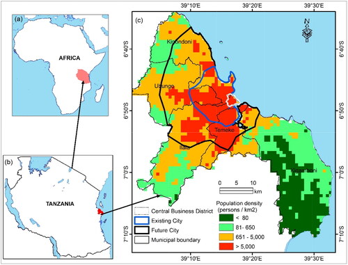
Economically, DMC is Tanzania’s port hub, commercial capital, and national centre of business, education, and culture. Continuous urban development has been associated with considerable LULC changes since the 1990s (Mkalawa 2016; Peter and Yang 2019). In addition, from 1998 to 2014, 17.55% of the city was transformed into high-and medium/low-density built-up areas (Mzava et al. 2019), largely driven by population expansion, economic growth, and greater infrastructural demand (Mkalawa and Haixiao 2014). Likewise, Tanzania marked a significant milestone in July 2020, when it formally moved from low-income to lower-middle-income country status after two decades of sustained progress. Tanzania’s success can be attributed to the country’s long-term financial stability, which has fuelled prosperity, as well as the country’s abundant natural resources and strategic geographic location (https://www.worldbank.org/en/country/tanzania/overview). Therefore, the abundant economic resources will likely be translated into urban infrastructure in its Metropolitan City.

Data collection and pre-processing

Two images from Landsat 5 Thematic Mapper (TM; 1995 and 2009) and one from Landsat 8 Operational Land Imager (OLI; 2017) were used to assess the relationships between LST and biophysical variables (NDBI, NDBaI, and SAVI) (Table 1). All images were acquired from the United States Geological Survey (https://earthexplorer.usgs.gov) for June and July. Images from the same month and interval could not be obtained due to heavy cloud cover.

Table 1. Details of Landsat satellite imagery.

Sensor	Path	Raw	Date of Acquired
Landsat 5 (TM)	166	65	25 June 1995
Landsat 5 (TM)	166	65	01 July 2009
Landsat 8 (OLI)	166	65	25 June 2017

Image pre-processing was implemented using Google Earth Engine open source code function for cloud, shadow, snow masking for Landsat 5 images (Ermida et al. 2020). The pre-processing includes stacking individual bands, cloud masking (for the 1995 image), radiometric correction, and clipping the stack to the study areas. Namely, cloud masking and gap-filling were completed using the Quality Assessment bands. The final images were exported to the Universal Transverse Mercator (UTM) coordinate system Zone 37 South, Spheroid Clarke 1880 and Datum Arc1960, specific for East Africa. Band math in ArcGIS v.10.8 was used to calculate LST and the derived spectral indices.

Variables extraction

LST

LST was estimated by applying structured mathematical algorithms reliant upon the thermal infrared bands and their respective mean differences in land surface emissivity (Rongali et al. 2018). LST extraction involved two steps: conversion to at-sensor spectral radiance and changing the spectral value of radians to the at-satellite brightness temperature. Achieving a standard radiometric scale required calculating the at-sensor spectral radiance. Further calibrations were essential for all Landsat images acquired from all sensors and were achieved by converting raw digital numbers (DNs) from satellites to digital numbers with the same radiometric scaling (Chander et al. 2009). For Level 1 Landsat products, the calibrated digital number (QC) was converted to the at-sensor spectral radiance (Lλ) using Eq. 1(1) $$L\lambda =\frac{\mathit{Lmax}\lambda -\mathit{Lmin}\lambda }{\mathit{QCalmax}-\mathit{QCalmin}}\mathrm{*}\left(\mathit{QCal}-\mathit{QCalmin}\right)+\mathrm{L}\min \lambda$$(1) (Kashki et al. 2021): (1) $$L\lambda =\frac{\mathit{Lmax}\lambda -\mathit{Lmin}\lambda }{\mathit{QCalmax}-\mathit{QCalmin}}\mathrm{*}\left(\mathit{QCal}-\mathit{QCalmin}\right)+\mathrm{L}\min \lambda$$(1) where Lλ is the spectral radiance at the sensor’s aperture (W·m⁻²·sr⁻¹·μm⁻¹), QCal is the quantified calibrated pixel value (DN), Qcalmin is the minimum quantised calibrated pixel value corresponding to Lmin_λ (DN), Qcalmax is the maximum quantised calibrated pixel value corresponding to Lmax_λ (DN), Lmin_λ is the spectral at-sensor radiance scaled to Qcalmin (W·m⁻²·sr⁻¹·μm⁻¹), and Lmax_λ is the spectral at-sensor radiance scaled to Qcalmax (W·m⁻²·sr⁻¹·μm⁻¹).

The second step involved changing the spectral value of radians to the at-sensor brightness temperature (Tb; °C) after converting DNs to spectral radiance (Eq. 2(2) $$b=\frac{K_2}{ln\left(\left(\frac{K_1}{L_{\lambda }}\right)+1\right)}-273.15$$(2) ): (2) $$b=\frac{K_2}{ln\left(\left(\frac{K_1}{L_{\lambda }}\right)+1\right)}-273.15$$(2) where K₁ and K₂ are the calibration constants of thermal bands.

The differences in Earth’s surface conditions can be attributed to large-scale thermal fluctuations of the land surface properties, where variations in vegetation coverage, surface wetness, roughness, and viewing angles contribute to differences in land surface emissivity (Yu et al. 2014). Accordingly, the land surface temperature was further modified using the land surface emissivity (ε_ƛ; Zhao et al. 2018) via Eq. (4)(4) $$\mathrm{\epsilon }\mathrm{ }=\mathrm{ }0.\mathrm{ }004\text{ * }{P}_V\mathrm{ }+\mathrm{ }0.\mathrm{ }986$$(4) : (3) $$T_s=\frac{Tb}{\left\{\left.1+⌊\left(\lambda BT/p\right)ln{\epsilon }_{\mathrm{ƛ}}⌋\right\}\right.}$$(3) where T_s is the LST (°C); Tb is the at-sensor temperature (°C); λ is the effective wavelength of emitted radiance (≈11.5 μm), equal to hc/σ = 1.438 × 10⁻² mK,here, σ is the Boltzmann constant (1.38 × 10⁻²³ J·K⁻¹), h is Planck’s constant (6.626 × 10⁻³⁴ Js), and c is the speed of light (2.998 × 10⁸ m·s⁻¹); and ε_λ is the emissivity, as calculated by Barsi et al. (2014) using Eq. 4(4) $$\mathrm{\epsilon }\mathrm{ }=\mathrm{ }0.\mathrm{ }004\text{ * }{P}_V\mathrm{ }+\mathrm{ }0.\mathrm{ }986$$(4) : (4) $$\mathrm{\epsilon }\mathrm{ }=\mathrm{ }0.\mathrm{ }004\text{ * }{P}_V\mathrm{ }+\mathrm{ }0.\mathrm{ }986$$(4) where P_V is the proportion of vegetation, as calculated via Eq. 5(5) $$P_v={\left(\frac{\mathit{NDVI}-{\mathit{NDVI}}_{\min }}{{\mathit{NDVI}}_{\max }-{\mathit{NDVI}}_{\min }}\right)}^2$$(5) : (5) $$P_v={\left(\frac{\mathit{NDVI}-{\mathit{NDVI}}_{\min }}{{\mathit{NDVI}}_{\max }-{\mathit{NDVI}}_{\min }}\right)}^2$$(5) where NDVI is the normalised difference vegetation index calculated from the red and near-infrared bands of Landsat images.

Variable selection and derivation

LST is affected by various variables, including topographic conditions, climatic and atmospheric factors, and vegetation (Kashki et al. 2021). Here, three biophysical variables representing vegetation (agricultural land, shrubland, forest, and grassland), bare soil, and built-up areas (buildings, roads, and other impervious surfaces) were selected based on prior LULC knowledge of the region. Accordingly, three indices: SAVI, NDBaI, and NDBI, were generated as explanatory variables for assessing the modelling of biophysical variables and land surface temperatures across DMC (Table 2).

Table 2. Derivation of spectral index explanatory variables from Landsat data.

Spectral Index	Expression	Reference
NDBaI	(SWIR1-TIRS)/(SWIR1+TIRS)	(Zhao and Chen 2005)
SAVI	((NIR-RED)/(NIR + RED))*(1+L)	(Huete 1988)
NDBI	(SWIR1-NIR)/(SWIR1+NIR)	(Zha et al. 2003)

Normalised difference bareness index (NDBaI)

NDBaI was chosen to represent bare land areas, which often display considerable variation in thermal characteristics (Sun et al. 2012). The index was estimated using the reflectance of the middle infrared (band 5 for Landsat 5 and 7 and band 6 for Landsat 8) and thermal infrared (band 6 for Landsat 5 and 7 and bands 10 and 11 for Landsat 8) bands according to Eq. 6(6) $$\mathit{NDBaI}=\frac{\mathit{MIR}-\mathit{TIR}}{\mathit{MIR}+\mathit{TIR}}.$$(6) : (Zhao and Chen 2005) (6) $$\mathit{NDBaI}=\frac{\mathit{MIR}-\mathit{TIR}}{\mathit{MIR}+\mathit{TIR}}.$$(6)

Soil-adjusted vegetation index (SAVI)

SAVI employs a soil-brightness correction factor for minimising the influence of soil brightness and was calculated via Eq. 7(7) $${\mathit{SAVI}}_{.}={\left(\frac{\mathit{NIR}-\mathrm{RED}}{\mathit{NIR}+\mathit{RED}}\right)\mathrm{*}(1+L)}^{,}$$(7) (Huete 1988): (7) $${\mathit{SAVI}}_{.}={\left(\frac{\mathit{NIR}-\mathrm{RED}}{\mathit{NIR}+\mathit{RED}}\right)\mathrm{*}(1+L)}^{,}$$(7) where NIR, RED, and L represent the near-infrared band, red band, and L-correlation factor, respectively. Notably, non-vegetated urban areas often produce abundant soil reflectance values (Hidayati et al. 2018). The L-correlation factor varied depending on the density of vegetation cover, where low and high densities produced an L value of 1 and ∼0.25, respectively. As low- to high-density vegetation cover in observed across the study area, a correction factor of L = 0.5 was applied (Huete 1988; Kaspersen et al. 2015).

Normalised difference built-up index (NDBI)

NDBI was developed to identify urban built-up areas and produces values from −1 to 1; where a negative NDBI represents water bodies and higher values represent built-up areas via Eq. 8(8) $${\mathit{NDBI}}_{.}={\left(\frac{{\mathit{SWIR}}_1-\mathit{NIR}}{{\mathit{SWIR}}_1+\mathit{NIR}}\right)}^{.}$$(8) (Zha et al. 2003): (8) $${\mathit{NDBI}}_{.}={\left(\frac{{\mathit{SWIR}}_1-\mathit{NIR}}{{\mathit{SWIR}}_1+\mathit{NIR}}\right)}^{.}$$(8) where SWIR is the short-wave infrared and NIR is the near-infrared band.

Spatial sampling data

All dependent variables and predictors were initially raster layers with a spatial resolution of 30 m; therefore, the rasters were entirely transformed into vector and tabular data, as required by the R-based GWR, according to the following steps: first, considering the size of the original data as well as the reduction of spatial autocorrelation, 1 × 1 km regular grids were created within the study region based on descriptive studies at the megacity level (Li et al. 2010; Zhao et al. 2018) in ArcGIS. Next, values for the original dependent and explanatory variables in raster format were extracted from each grid and exported to a spreadsheet. After removing the incomplete data, ∼1600 data points remained for use in the GWR model.

Ordinary least square and geographically weighted regression models

Ordinary least square (OLS)

OLS is based on the assumption that the sample regression model is closest to the observations. In OLS spatial modelling, the coefficients or statistical model parameters are assumed constant; thus, this model estimated a similar value for dependent variables across the entire research area, a notable limitation during spatial modelling (Deilami et al. 2016). The OLS coefficient matrix was calculated according to Eq. 9(9) $$\mathrm{y}\mathrm{ }=\mathrm{ }X\beta \mathrm{ }+\mathrm{ }\epsilon$$(9) : (9) $$\mathrm{y}\mathrm{ }=\mathrm{ }X\beta \mathrm{ }+\mathrm{ }\epsilon$$(9) where y is the estimated dependent variable, x is the estimator, and ε is the model error or deviation when estimating β or model coefficients (Kashki et al. 2021).

Geographically weighted regression (GWR)

GWR is a nonstationary local regression technique that calculates the relationship between a dependent variable and its explanatory variables at each sample point (Kashki et al. 2021). Unlike a conventional (global) regression model, GWR adds one or more geographic parameters to traditional global regression (Ahmadi et al. 2018), enabling it to model spatial variation. The GWR model was calculated according to Eq. 10(10) $$y_i={\beta }_0(u_0,v_i+{\sum }_{I=1}^n{\beta }_n\left(u_i,v_i\right)x_{in}+{\Theta }_{i,}$$(10) : (10) $$y_i={\beta }_0(u_0,v_i+{\sum }_{I=1}^n{\beta }_n\left(u_i,v_i\right)x_{in}+{\Theta }_{i,}$$(10) where y_i is the observed variable; β₀ (u_i, v_i) is the regression constant of the sample point at (u_i, v_i); Βn (u_i, v_i) is the regression parameter, and is a function of the geographic location of variable n at the sample point; n is the number of factors; x_in is the value of the independent variable x_n at the sample point; and θ_i is the random error.

Observations were weighted according to their geographic distance to specific point i (i.e. the distance between an observation and point i determined its weight). To estimate the parameters in Eq. 11(11) $$\widehat{\beta }(u_i{v}_i)={\left(X^{T}W(u_i,v_i)X\right)}^{-}{}^1{X}^{T}W(u_i,v_i)y,$$(11) , the matrix equations were solved as follows: (11) $$\widehat{\beta }(u_i{v}_i)={\left(X^{T}W(u_i,v_i)X\right)}^{-}{}^1{X}^{T}W(u_i,v_i)y,$$(11) where X is the matrix of the independent variables with a column of 1 s for the intercept; y is the dependent variable vector; ${{\beta }_i={(\beta }_{i0}\dots .{\beta }_{im})}^T$ is the vector of m + 1 local regression coefficients; Wi is the diagonal matrix denoting the geographical weighting of each observed data for regression point I; and W(ui, vi) is the weighting matrix, ensuring that observations closer to a given location maintain more weight than more distant locations. Further, this study utilised the Gaussian weighted kernel function (Eq. 12(12) $$w_{ij}=\exp (-\beta \frac{d_{ij}^2}{b^2})$$(12) ): (12) $$w_{ij}=\exp (-\beta \frac{d_{ij}^2}{b^2})$$(12) where d_ij is the Euclidean distance between regression point i and nearby observation j and b denotes the basal width of the kernel function (i.e. bandwidth). If j corresponds to i in Eq. 11(11) $$\widehat{\beta }(u_i{v}_i)={\left(X^{T}W(u_i,v_i)X\right)}^{-}{}^1{X}^{T}W(u_i,v_i)y,$$(11) , the weighting value of the data at that location was set to 1; whereas wij decreased with increasing distance according to a Gaussian curve (Brunsdon et al. 1996; Shi et al. 2006).

Coefficient of determination (R2)

The coefficient of determination (R²) was used to assess the model fit and was derived by comparing estimated and observed values. Here, R² values vary from 0 to 1, where higher values indicate a more perfect fit, as it denotes the proportion of variance in the dependent variable explained by the independent variable(s) (Li et al. 2010; Luo and Peng 2016).

Akaike information criterion (AIC)

The Akaike information criterion (AIC) is a mathematical technique used in statistics to determine model fit by creating a compromise between model accuracy and complexity, where a low value suggests that the model’s predicted value is closer to the observed value or reality (Li et al. 2010; Kashki et al. 2021).

Spatial autocorrelation by global Moran’s I index

The global Moran’s I index was used to check whether the explanatory variables were independent of each other (i.e. not spatially autocorrelated). Moran’s I can be classified as positive, negative, or without spatial autocorrelation. Here, positive autocorrelation occurs when similar values are clustered together in space and negative spatial autocorrelation when similar values are dispersed. 0 values represent perfect randomness.

OLS and GWR statistical analyses

Using the OLS and GWR models, the spatial relationships between LST and LULC biophysical variables were obtained. First, a correlation coefficient analysis was used to ensure that the predictor variables were statistically significant for GWR modelling (Gregorich et al. 2021). To this end, a variance inflation factor (VIF) was calculated to ensure the lack of multicollinearity between NDBI, NDBaI, and SAVI (Zhi et al. 2020). Conventionally, explanatory variables with VIF values > 7.5 were considered highly correlated and were removed from regression models (Li et al. 2010). All analyses were performed with a significance level of p < 0.01 and diagnostics of the regression models were conducted in R v4.2.1 using the spgwr package. All maps were produced in ArcGIS.

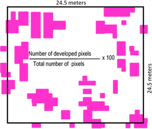
Building density pixel mapping

Actual building layers for the research locations were required to appropriately map building densities. Here, the Dar es Salaam building layer for 2016 was downloaded from Resilience Academy (https://resilienceacademy.ac.tz) and updated using high-resolution imagery from Google Earth to match the LSTs for 2017. Utilising the neighborhood analysis tool in ArcGIS, built-up pixels were divided into high-, moderate-, and low-density categories based on the number of built-up pixels present in the high-density plot, which maintains a plot size of 301–600 m,² with a maximum of one household, two buildings per plot, and a maximum plot coverage of 60% (URT 2018). Based on the typical standards of urban residential areas, the cut-off percentages for low- and moderate-densities were somewhat arbitrary, as they relied heavily upon researchers’ judgment. Subsequently, each built-up pixel in the plot was subjected to an "If" condition to determine density characters levels, as follows:

• High-density pixels are built-up, surrounded by ≥ 30% of other built-up pixels;

• Moderate-density pixels are built-up, surrounded by 10–30% of other built-up pixels;

• Low-density pixels are built-up, surrounded by < 10% of other built-up pixels.

The concept of determining the built-up pixels in the urban high-density plot with an arbitrary plot area of 600m2 is presented in Figure 2.

Results

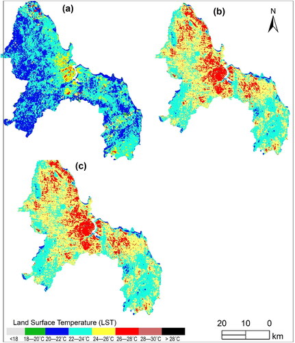
Spatiotemporal variability in land surface temperature

The spatiotemporal variability of LSTs in 1995, 2009, and 2017 are displayed in Figure 3. The results indicated that the LST minimum temperatures were 16.55, 16.56, and 14.55 and the and maximum temperatures were 27.95, 50.29, and 31.47 °C for 1995, 2009, and 2017, respectively, with mean LSTs of 22.37, 22.43, and 25.32 °C. As a result, the area with higher temperatures appeared to increase compared to previous years, as the mean LST decreased by 0.06 °C between 1995 and 2009 but increased by 2.30 °C from 2009 to 2017. While the highest LST (> 28 °C) was recorded in the city’s eastern portion, near the CBD, the western and southwestern parts maintained the lowers LSTs (< 22 °C).

Figure 2. Concept of determination for built-up pixels in the urban high-density plot.

Spatial distribution of three biophysical parameters

The spatial distributions of the three biophysical variables are shown in Figure 4. Namely, the eastern and central areas displayed the higher NDBI values than the western and southern areas, that contained few or no buildings. Alternatively, the SAVI map (Figure 4b) shows that the western and southern regions maintained higher values compared to the eastern and central regions, where structures occupy larger areas. On the western side, larger SAVI values were related to the presence of game reserves, primarily woodland forests. The highest NDBaI (Figure 4c) values were maintained at the western side of the study region, in contrast to the central and eastern regions that contained much more limited areas covered by bare soil.

Figure 3. Spatiotemporal distribution of LST for (a) 1995, (b) 2009, and (c) 2017.

GWR and OLS analysis of driving factors

OLS analysis of driving factors

The regression parameters of LST established by OLS are indicated in Table 3. Notably, OLS results were less than ideal, producing an R² = 0.4323 and Moran’s I ≤ 0.66. According to Table 4, the VIF values of all explanatory variables were < 7.5, except for the NDBaI and NDBI of 2009, indicating the lack of collinearity among these variables. Moreover, OLS model coefficients for all years, except NDBaI for 2009, were statistically significant (p < 0.05). Accordingly, due to its high collinearity with NDBI and lack of statistical significance, NDBaI was excluded from GWR modelling in 2009.

Table 3. OLS model regression results.

	1995	2009	2017
Multiple R^2	0.3593	0.352	0.4334
Adjusted R^2	0.3581	0.3508	0.4323

Table 4. Regression coefficients between LST and driving factors.

	1995			2009			2017
	NDBI	SAVI	NDBaI	NDBI	SAVI	NDBaI	NDBI	SAVI	NDBaI
Correlation	3.54***	−2.32***	0.77**	5.13***	−2.36***	1.24*	4.11***	−2.88***	−2.14***
VIF	3.32	1.76	2.95	9.80	4.38	7.28	5.18	4.83	2.91
Intercept	23.87***			23.10***			26.37***

significance level (p-value): ^*** p < 0.001; ^** p < 0.01; ^* p < 0.05

Geographical weighted regression (GWR) analysis of driving factors

The spatial variation of LSTs were analysed using the GWR model and all three biophysical variables. Table 5 presents a summary of the analysis. The corrected AIC (AICc) values were the lowest in 2009, indicating that the values predicted by the model were closer to those observed in other years. As the cells were distributed regularly and consistently throughout the region, a fixed-kernel method was employed, producing maximum adjusted R² values between LST and the biophysical parameters of 0.55, 0.62, and 0.82 for 1995, 2009, and 2017, respectively.

Table 5. Results of modelling biophysical variables and LST by the GWR model.

^AICC	R^2	W^ARNING	Adjusted R^2	Unbiased sigma	Sigma biased
1995	3450.55181	0.64	0.55	0.7224467	0.7083403
2009	2983.044	0.89	0.82	0.6364869	0.6096698
2017	3535.6852	0.76	0.62	0.7166683	0.6892951

GWR and OLS spatial autocorrelation analysis using global Moran index

The spatial autocorrelation analysis of the global Moran’s I using the OLS and GWR models are presented in Table 6. Here, the Moran index values for OLS were higher (0.26, 0.66, and 0.21) than those for GWR (0.003, 0.14, and 0.07) in 1995, 2009, and 2017, respectively. Given the z-score values of 16–38 (OLS) and 3–8 (GWR) and variance values close to 0.000009, it was concluded that there was < 1% likelihood that this clustered pattern resulted from random chance; thus, the null hypothesis was accepted. Accordingly, it was concluded that the changes in LST over the DMC followed a random pattern.

Table 6. Global Moran’s I spatial autocorrelation summary for 1995, 2009, and 2017.

	1995		2009		2017
	OLS	GWR	OLS	GWR	OLS	GWR
Moran’s Index	0.296624	0.002755	0.660033	0.140143	0.212436	0.066100
Expected Index	−0.000646	−0.00065	−0.000560	0.000560	−0.000633	−0.000633
Variance	0.000185	0.000187	0.000297	0.000297	0.000176	0.000176
z-score	21.878568	0.248839	38.30695	8.166103	16.075018	5.034156
p-value	0.000000	0.803486	0.000000	0.000000	0.000000	0.000000

Modelling the impacts of biophysical variables on LST in DMC via GWR

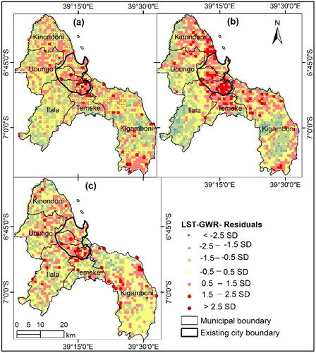
Owing to its ability to improve the understanding of LSTs and correlated biophysical variables throughout DMC, the GWR model was used to provide insight into the effects of biophysical variables on LST across the study area. Accordingly, the standard deviations of the residual values (the difference between the observed and predicted LST values) were calculated for 1995, 2009, and 2017 (Figure 5). The highest residual values were primarily observed in the existing city, whereas adjacent areas with compact human settlements indicated an increased built-up area. In addition, LST decreased with increasing vegetation.

Figure 4. Geographical variables affecting LST in the study area: a) NDBI, b) SAVI, and c) NDBaI.

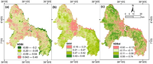
Figure 5. Distribution of residuals using GWR in the study area for a) 1995, b) 2009, and c) 2017.

Building density and LST

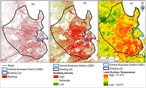
Maps of the study area’s existing city and CBD identifying high-, moderate-, and low-density pixels and their corresponding LSTs are shown in Figure 6. In the existing city area, high-density pixels constituted the majority of built-up pixels, followed by moderate- and low-density pixels. Although completed via visual inspection, high-density pixels corresponded closely to high LSTs in the existing city periphery; however, the LSTs of CBD containing high-rise and super high-rise buildings were lower than that of the adjacent current city.

Figure 6. Relationships between building density and LSTs in Dar es Salaam central business district and existing city: a) building layer, b) building density pixel classification, and c) LST. Building layer was modified from Resilience Academy - Dar es Salaam buildings (https://resilienceacademy.ac.tz).

Discussion

The results revealed that the LST dispersion in DMC appears to have increased dramatically over the past two decades. Notably, high LSTs were most frequent in the 'existing city’ area adjacent to the eastern CBD, owing to high building densities and low-rise buildings. This largely resulted from the decrease in vegetation, associated with the high rate of activities in the built-up areas in addition to the improvement of the transport sector, particularly road infrastructure (e.g. Dar es Salaam Rapid Transport) and higher building densities with low-to medium-rise buildings compared to other locations. Alternatively, low LSTs were observed in the west and southwest, probably due to thick vegetation in these areas, particularly in the Pande Game reserve. Typically, LSTs of areas with high-rise and super high-rise buildings are lower than that of areas with mid-rise buildings, which can be attributed to the large number of corresponding shadows (Yin et al. 2022). These findings are consistent with those of previous studies (Singh et al. 2017; Guha et al. 2018; Tarawally et al. 2018; Kashki et al. 2021). Uncontrolled LULC change especially that related to the growth of informal settlements leads to increasing urban densities, which in turn leads to higher LSTs; thus, it was concluded here that the urban pattern of high-density built-up areas can be upgraded to optimise the overall effects of the thermal environment.

The regression analyses revealed that built-up areas were more significantly correlated to higher LSTs across the DMC compared to other biophysical variables. Here, regression coefficients were both positive and negative, indicating spatial heterogeneity; whereas alternative patterns were observed in vegetated areas, as indicated by the slightly negative local regression coefficients of SAVI. The building area increased, which increased LSTs since built-up features absorb more sunlight, whereby thermal inertia is higher at impermeable levels (Zhang et al. 2017). Furthermore, vegetation is essential for reducing LSTs and heat islands in DMC due to its function as a natural air conditioning system that absorbs solar energy and transports water through its leaves into the atmosphere (Kashki et al. 2021); thus, it was observed here that this index was the most important factor influencing LSTs.

Nevertheless, the lower R² value observed in 1995 was probably explained by the local air turbulence and the presence of pressure systems, thereby reducing the effect of surface cover on temperature (Table 6; Alibakhshi et al. 2020).

Similarly, the correlations between LST and biophysical variables in this study confirmed that the choice of regression model considerably influenced the factor correlation analysis results. Namely, the analyses revealed that GWR outperformed the OLS global regression model, as indicated by the higher R² and AIC and lower spatial autocorrelation according to the Global Moran’s I. Notably, similar observations were reported in Xigang District of Northeast China by Zhi et al. (2020). Hence, GWR was more adaptable for predicting LSTs by incorporating the local and spatial features of variables across DMC. Moreover, OLS is unable to accurately examine the relationship between independent and dependent variables, even when correlations are positive in one section of the research area and negative in another (Kashki et al. 2021). It has also been noted elsewhere that the GWR works best with spatially connected variables as it allows for the investigation of spatial variation and displays model results as rasters (Kashki et al. 2021). Accordingly, GWR is a useful tool for investigating the spatial variation and interactions of different variables for decision-making purposes. For partitioned regional landscape design, nonstationary GWR modelling can provide locally detailed differentiation of the underlying mechanisms influencing LSTs. Thus, land use planning that addresses building densities to mitigate high LST effects, as well as the location and structure of green spaces in urban areas, are site-specific policies aimed at effective LST mitigation (Zhao et al. 2018). Furthermore, GWR can offer a more dynamic approach to parameter estimation than traditional regression methods using neighbourhood data, whereas OLS may not accurately identify LST variations over a diversified metropolitan landscape.

Study limitations

There were a few limitations in this study. For example, inconsistencies in the acquisition time of input data for modelling produced uncertainties. In addition, the study area is under cloud cover throughout much of the year. Hence, it was impossible to get clear sky images at regular intervals.

Conclusion and recommendations

According to GWR analysis, land cover and its correlated biophysical parameters profoundly influenced the LSTs of DMC, as determined through the high R² values. Therefore, it is essential to continuously monitor LULC change and quantify the relationships between LST and biophysical variable indices, such as NDBI, NDWI, SAVI, and NDBaI. Furthermore, environmental specialists, urban planners, and other officials should prioritise the GWR model when formulating location-specific LST mitigation strategies. Further research is recommended into modelling the relationships between LST and other variables, such as climate, wind, solar radiation, population density, and topography.

Acknowledgements

The authors would like to thank the National Aeronautics and Space Administration (NASA) and United States Geological Survey (USGS) for providing the entire Landsat imagery, as well as the Ministry of Lands, Housing, and Human Settlement Development, and the National Bureau of Statistics of Tanzania for providing the administrative boundaries of the study area.

Disclosure statement

No potential conflict of interest was reported by the authors.

Data availability statement

The data that support the findings of this study are available from the corresponding author, [O.S], upon reasonable request.

References

- Afrakhteh R, Asgarian A, Sakieh Y, Soffianian A. 2016. Evaluating the strategy of integrated urban-rural planning system and analysing its effects on land surface temperature in a rapidly developing region. Habitat Int. 56:147–156.
- Ahmadi M, Kashki AR, Dadashi Roudbari AA. 2018. Spatial modeling of seasonal precipitation–elevation in Iran based on Aphrodite database. Model Earth Syst Environ. 4(2):619–633.
- Alhowaish AK. 2015. Eighty years of urban growth and socioeconomic trends in Dammam Metropolitan Area, Saudi Arabia. Habitat Int. 50:90–98.
- Alibakhshi Z, Ahmadi M, Farajzadeh Asl M. 2020. Modeling biophysical variables and land surface temperature using the GWR model: case study—Tehran and its satellite cities. J Indian Soc Remote Sens. 48(1):59–70.
- Barsi JA, Lee K, Kvaran G, Markham BL, Pedelty JA. 2014. The spectral response of the Landsat-8 operational land imager. Remote Sens. 6(10):10232–10251.
- Baruti MM, Johansson E, Yahia MW. 2020. Urbanites’ outdoor thermal comfort in the informal urban fabric of warm-humid Dar es Salaam, Tanzania. Sustain Cities Soc. 62(July):102380.
- Brunsdon C, Fotheringham AS, Charlton M. 1996. Geographically weighted regression: a method for exploring spatial nonstationarity. . 28(4):285–287.
- Chander G, Markham BL, Helder DL. 2009. Summary of current radiometric calibration coefficients for Landsat MSS, TM, ETM+, and EO-1 ALI sensors. Remote Sens Environ. 113(5):893–903.
- Chen S, Yu Z, Liu M, Da L, Faiz M. 2021. Trends of the contributions of biophysical (climate) and socioeconomic elements to regional heat islands. Sci Rep. 11(1):14.
- Deilami K, Kamruzzaman M, Hayes JF. 2016. Correlation or causality between land cover patterns and the urban heat island effect? Evidence from Brisbane, Australia. Remote Sens. 8(9):716.
- Ermida SL, Soares P, Mantas V, Göttsche FM, Trigo IF. 2020. Google earth engine open-source code for land surface temperature estimation from the landsat series. Remote Sens. 12(9):1471.
- Esha EJ, Ahmed A. 2018. Impacts of land use and land cover change on surface temperature in the north-western region of Bangladesh. 5th IEEE Reg 10 Humanitarian Technology Conference 2017, R10-HTC 2017; p. 200523.
- Fan C, Rey SJ, Myint SW. 2017. Spatially filtered ridge regression (SFRR): a regression framework to understanding impacts of land cover patterns on urban climate. Trans in GIS. 21(5):862–879.
- Firozjaei MK, Alavipanah SK, Liu H, Sedighi A, Mijani N, Kiavarz M, Weng Q. 2019. A PCA-OLS model for assessing the impact of surface biophysical parameters on land surface temperature variations. Remote Sens. 11(18):2094.
- Fonseka HPU, Zhang H, Sun Y, Su H, Lin H, Lin Y. 2019. Urbanisation and its impacts on land surface temperature in Colombo Metropolitan Area, Sri Lanka, from 1988 to 2016. Remote Sens. 11(8):957.
- Gohain KJ, Mohammad P, Goswami A. 2021. Assessing the impact of land use land cover changes on land surface temperature over Pune city, India. Quat Int. 575–576:259–269.
- Gregorich M, Strohmaier S, Dunkler D, Heinze G. 2021. Regression with highly correlated predictors: variable omission is not the solution. IJERPH. 18(8):4259.
- Gu C. 2019. Urbanisation: processes and driving forces. Sci China Earth Sci. 62(9):1351–1360.
- Guha S, Govil H, Dey A, Gill N. 2018. Analytical study of land surface temperature with NDVI and NDBI using Landsat 8 OLI and TIRS data in Florence and Naples city, Italy. Eur J Remote Sens. 51(1):667–678.
- Guha S, Govil H, Gill N, Dey A. 2020. Analytical study on the relationship between land surface temperature and land use/land cover indices. Ann GIS. 26(2):201–216.
- Hidayati IN, Suharyadi R, Danoedoro P. 2018. Developing an extraction method of urban built-up area based on remote sensing imagery transformation index. For Geo. 32(1):96–108.
- Huete AeR. 1988. A soil-adjusted vegetation index (SAVI). Remote Sens Environ. 25(3):295–309.
- Kabanda T. 2019. Urban heat island analysis in Dar es Salaam. Tanzania. S Afr J Geom. 8(1):98–107.
- Kafy A-A, Rahman MS, Faisal A, Hasan MM, Islam M. 2020. Modelling future land use land cover changes and their impacts on land surface temperatures in Rajshahi, Bangladesh. Remote Sens Appl Soc Environ. 18(March):100314.
- Kashki A, Karami M, Zandi R, Roki Z. 2021. Evaluation of the effect of geographical parameters on the formation of the land surface temperature by applying OLS and GWR, A case study Shiraz City, Iran. Urban Clim. 37:100832.
- Kaspersen PS, Fensholt R, Drews M. 2015. Using Landsat vegetation indices to estimate impervious surface fractions for European cities. Remote Sens. 7(6):8224–8249.
- Kibassa D, Shemdoe R. 2016. Land cover change in urban morphological types of Dar es Salaam and its implication for green structures and ecosystem services. MESE. 2(3):171–186.
- Lafortezza R, Sanesi G. 2019. Nature-based solutions: settling the issue of sustainable urbanisation. Environ Res. 172(August 2018):394–398.
- Li S, Zhao Z, Miaomiao X, Wang Y. 2010. Investigating spatial non-stationary and scale-dependent relationships between urban surface temperature and environmental factors using geographically weighted regression. Environ Modell Softw. 25(12):1789–1800.
- Livesey N. 2014. Limb sounding atmospheric. In: Njoku EG, editor. Encyclopedia of remote sensing in encyclopedia of earth sciences series. New York, NY: Springer.
- Luo X, Peng Y. 2016. Scale effects of the relationships between urban heat islands and impact factors based on a geographically weighted regression model. Remote Sens. 8(9):760.
- Malekela AA, Nyomora A. 2019. Climate change: its implications on urban and peri-urban agriculture in Dar es Salaam city. Tanzania. Sci Devel J. 3(1):1–14.
- Manyama MT, Nahonyo CL, Hepelwa AS. 2020. Analysis of the impact of built environment on coastline ecosystem services and values. East Afr J Environ Nat Resour. 2(2):44–63.
- Mkalawa CC. 2016. Analysing Dar es Salaam urban change and its spatial pattern. Int J Urban Plan Transp. 31(1):1138–1149.
- Mkalawa CC, Haixiao P. 2014. Dar es Salaam city temporal growth and its influence on transportation [accessed June 2016]. Urban Plann Transport Res. 2(1):423–446.
- Mzava P, Nobert J, Valimba P. 2019. Land cover change detection in the urban catchments of Dar es Salaam, Tanzania using remote sensing and GIS techniques. Tanzania J Sci. 45(3):315–329. www.ajol.info/index.php/tjs/.
- Nanjing T, Wang R, Hou H, Murayama Y. 2020. Spatiotemporal analysis of land use/cover patterns and their relationship with land surface. Remote Sens. 1:1–17.
- Nasir MJ, Ahmad W, Iqbal J, Ahmad B, Abdo HG, Hamdi R, Bateni SM. 2022. Effect of the urban land use dynamics on land surface temperature: a case study of Kohat City in Pakistan for the period 1998–2018. Earth Syst Environ. 6(1):237–248.
- Orimoloye IR, Mazinyo SP, Nel W, Kalumba AM. 2018. Spatiotemporal monitoring of land surface temperature and estimated radiation using remote sensing: human health implications for East London, South Africa. Environ Earth Sci. 77(3):1–10.
- Peng J, Xie P, Liu Y, Ma J. 2016. Urban thermal environment dynamics and associated landscape pattern factors: A case study in the Beijing metropolitan region. Remote Sens Environ. 173:145–155.
- Peter LL, Yang Y. 2019. Urban planning historical review of master plans and the way towards a sustainable city: Dar es Salaam, Tanzania. Front Archit Res. 8(3):359–377.
- Rongali G, Keshari AK, Gosain AK, Khosa R. 2018. A mono-window algorithm for land surface temperature estimation from Landsat 8 thermal infrared sensor data: A case study of the Beas River Basin, India. Pertanika J Sci Technol. 26(2):829–840.
- Sekertekin A, Arslan N. 2019. Monitoring thermal anomaly and radiative heat flux using thermal infrared satellite imagery – A case study at Tuzla geothermal region. Geothermics. 78:243–254.
- Shi H, Zhang L, Liu J. 2006. A new spatial-attribute weighting function for geographically weighted regression. Can J for Res. 36(4):996–1005.
- Singh P, Kikon N, Verma P. 2017. Impact of land use change and urbanisation on urban heat island in Lucknow city, Central India. A remote sensing based estimate. Sustain Cities Soc. 32:100–114.
- Sun Q, Wu Z, Tan J. 2012. The relationship between land surface temperature and land use/land cover in Guangzhou, China. Environ Earth Sci. 65(6):1687–1694.
- Tarawally M, Xu W, Hou W, Mushore TD. 2018. Comparative analysis of responses of land surface temperature to long-term land use/cover changes between a coastal and Inland City: A case of Freetown and Bo Town in Sierra Leone. Remote Sens. 10(1):112–118.
- URT. 2013a. 2012 population and housing census: population distribution by administrative areas. Dar es Salaam: National Bureau of Statistics.
- URT. 2013b. Dar es Salaam Masterplan 2012 – 2032. Ministry of Lands, Housing and Human Settlement Development.
- URT. 2018. The Urban Planning Act (CAP. 355), The Urban Planning (Planning and Space Standards) Regulations.
- Wang R, Hou H, Murayama Y, Derdouri A. 2020. Spatiotemporal analysis of land use/cover patterns and their relationship with land surface temperature in Nanjing, China. Remote Sens. 12(3):440.
- Yin S, Liu J, Han Z. 2022. Relationship between urban morphology and land surface temperature-A case study of Nanjing City. PLoS ONE. 17(2):e0260205–17.
- Yu X, Guo X, Wu Z. 2014. Land surface temperature retrieval from Landsat 8 TIRS-comparison between radiative transfer equation-based method, split window algorithm and single channel method. Remote Sensing. 6(10):9829–9852.
- Zha Y, Gao J, Ni S. 2003. Use of normalised difference built-up index in automatically mapping urban areas from TM imagery. Int J Remote Sens. 24(3):583–594.
- Zhang X, Estoque RC, Murayama Y. 2017. An urban heat island study in Nanchang City, China based on land surface temperature and social-ecological variables. Sustain Cities Soc. 32:557–568.
- Zhao H, Chen X. 2005. Use of normalised difference bareness index in quickly mapping bare areas from TM/ETM. Int Geosci Remote Sens Symp. 3:1666–1668.
- Zhao M, Cheng C, Zhou Y, Li X, Shen S, Song C. 2022. A global dataset of annual urban extents (1992–2020) from harmonised nighttime lights. Earth Syst Sci Data. 14(2):517–534.
- Zhao C, Jensen J, Weng Q, Weaver R. 2018. A geographically weighted regression analysis of the underlying factors related to the surface urban heat island phenomenon. Remote Sens. 10(9):1428.
- Zhi Y, Shan L, Ke L, Yang R. 2020. Analysis of land surface temperature driving factors and spatial heterogeneity research based on geographically weighted regression model. Complexity. 2020:1–9.
- Zhou G, Wang H, Chen W, Zhang G, Luo Q, Jia B. 2020. Impacts of urban land surface temperature on tract landscape pattern, physical and social variables. Int J Remote Sens. 41(2):683–703.