Cloud detection using sentinel 2 imageries: a comparison of XGBoost, RF, SVM, and CNN algorithms

Abstract

This study reports results of the Extreme Gradient Boosting (XGBoost) algorithm in comparison to Random Forest (RF), Support Vector Machine (SVM), and Convolutional Neural Network (CNN) to generate cloud mask comprising of six classes: low cloud, high cloud, cloud shadow, ground, snow, and water. Here, Baetens-Hagolle dataset and WHUS2-CD dataset was considered. Various texture features derived using GLCM, morphological profile analysis, bilateral filtering, and deep features derived using Residual Network (Resnet) were used in combination with spectral information. The first phase of the study suggested both XGBoost and RF exhibit comparable performance for both traditional texture features and deep features, the second phase highlighted that XGBoost showed better generalization capabilities with respect to the different environmental conditions, and finally, comparison with threshold-based methods (Function of Mask [Fmask], Sen2cor, and Maccs-Atcor Joint Method [MAJA]) suggested that XGBoost and RF based cloud detection is a good alternative of existing state-of-the-art cloud detection.

Keywords:

• Cloud shadow
• detection
• Sentinel-2
• features
• machine learning

1. Introduction

Earth observation activities like land cover monitoring, climate change studies, agriculture monitoring, identification of crops and mapping, disaster management, urban growth assessment, military surveillance, mining resources, etc., are performed by analyzing optical imagery acquired by Earth-imaging satellites. These Earth imaging satellites (e.g. Sentinel 2, Landsat) commonly capture scenes by receiving sun energy which is reflected from Earth’s surface to space (i.e. Earth’s albedo). The imageries acquired by these satellites are freely available for Earth observation activities, which substantially boosted the demand for analysis-ready data. Images of the Earth’s surface are usually acquired by sensors at a fixed interval and are likely to be affected by the presence of clouds (Fritz 1949). There is a high probability of information loss as clouds are also likely to appear on the same scene when the sensor passes over the area again. Thus, cloud detection and screening become an important preprocessing part before using remote sensing images for further studies. About 67% of Earth’s surface is most often covered with clouds of different types like cirrus, cumulus, stratus, and nimbus (King et al. 2013). Clouds can be differentiated based on the properties like visibility, transparency, reflectance, brightness, height, shape, etc. (Arking and Childs 1985; Wang and Rossow 1995). Clouds are also categorized based on their height from Earth’s surface as low, medium, and high. Low clouds are found almost touching the ground and lie within 2 km above ground level (AGL), which usually comprise stratus, stratocumulus, and nimbostratus clouds which are formed by condensation of water droplets. Medium clouds are in between low and high clouds (2–6 km) that include altostratus and altocumulus clouds and are formed due to low temperatures by ice crystals and water droplets. High clouds are usually above 6 km, including cirrus, cirrostratus, and cirrocumulus clouds that are formed by ice crystals in the presence of stable air (Wang and Rossow 1995). On the basis of visibility, low clouds are typically brightest, Medium clouds are comparatively less bright, and high clouds usually are very thin and opaque (Mishchenko et al. 1996).

The process of determining cloud and cloud-free areas in satellite imagery is considered as cloud detection. The exact detection of cloud and cloud shadow in satellite imageries is a challenging task because clouds are usually mismatched with bright objects such as ice or snow, whereas cloud shadows with dark surface objects on Earth’s surface due to their spectral similarities (Irish 2000). In addition, each type of cloud exhibits different properties and signatures, like low and medium clouds are optically thick and hide Earth’s surface features, whereas high clouds are usually thin and make Earth’s surface look hazy (Le Hégarat-Mascle and André 2009). Cloud shadows are also different for each type of cloud, like the shadow of low and medium cloud is darkest, whereas high cloud shadow is almost the same as clear areas. The most reliable method of cloud detection used so far is the manual interpretation of satellite imagery, but it requires expert domain knowledge and is time-consuming. Keeping in view of this problem, an automated method of cloud detection, also known as automated cloud masking, has been proposed to substitute the manual method. Cloud masking is the process of assigning a fixed value to each pixel of a satellite image that helps in interpreting the image into different classes, that is cloud, shadow, clear, etc., and the file which stores the assigned value is called cloud mask. Mainly, there are two types of cloud masking techniques: threshold-based and machine learning-based (Tarrio et al. 2020). Most commonly used cloud masking methods are threshold-based approaches (single-date and multi-temporal). In these approaches, a threshold that separates cloud-free pixels from cloudy pixels over different spectral bands of satellite imagery is used. Single-date threshold-based methods generate masks by taking only the spectral bands of one particular image as input. In contrast, multi-temporal threshold-based methods consider time-series data of that particular image captured over a certain period (Zhu and Woodcock 2014). Single-date threshold-based methods perform better with lower threshold values but misclassify cloud-free pixels as cloud and shadow, leading to insufficient cloud-free data (Zhu and Woodcock 2014). The multitemporal threshold-based method compares time-series data to evaluate sudden changes in reflectance (Hagolle et al. 2010). The function of mask (Fmask) is considered the best single date threshold-based method whereas the Maccs-Atcor Joint Method (MAJA) is considered best for multitemporal data (Tarrio et al. 2020). These threshold-based methods require expert knowledge to select constant or dynamic threshold values.

Machine learning-based cloud detection methods such as Support Vector Machine (SVM), Random Forest (RF), Decision Tree, etc., are proposed and do not require a threshold value selection as in threshold-based methods. These methods consider the cloud detection problem as a pixel-wise classification problem, which either utilizes the concept of supervised learning, where predefined labeled pixels are used for training a classifier, or the concept of semi-supervised learning, in which classifier learns to group unlabeled pixels, which is then labeled into respective classes using small available pixel-wise information (Tapakis and Charalambides 2013). These classifiers can be trained with just one feature or several features. Features used for cloud detection can include spectral, texture, frequency, and other mathematically derived features like Normalized Difference Vegetation Index (NDVI), Normalized Difference Snow Index (NDSI), and Normalized Difference Water Index (NDWI), etc. Some important feature extraction techniques used to extract traditional texture features are Grey-level co-occurrence matrix (GLCM), Local Binary pattern (LBP), bilateral filtering, and morphological profiles. Among various machine learning approaches, SVM has extensively been used for cloud detection. A significant advantage of using SVM is their ability to achieve high accuracy with a smaller training sample size (Bai et al. 2016; Deng et al. 2019; Pérez-Suay et al. 2018; Joshi et al. 2019; Ibrahim et al. 2021; Li et al. 2022). The requirement of huge computational costs during training and testing when used with a large satellite dataset is found to be a major challenge with the SVM approach. On the other hand, RF-based cloud detection methods are much faster, can handle large image datasets, and achieve classification accuracy (Ghasemian and Akhoondzadeh 2018; Fu et al. 2018; Chen et al. 2020; Wei et al. 2020; Yao et al. 2022). Extreme Gradient Boosting (XGBoost) is another tree-based method that has proven to be highly efficient in dealing with large-scale data for remote sensing applications (Bhagwat and Shankar 2019; Zamani Joharestani et al. 2019; Rumora et al. 2020) but has not been explored for cloud detection problem.

Recently, convolutional neural network (CNN) based deep learning methods have also been used for cloud detection due to their ability to automatically extract low to high-level features by incorporating spatial characteristics for each pixel (Segal-Rozenhaimer et al. 2020; Ma et al. 2021). CNN utilizes spatial correlations that highlight cloud features usually distributed in the imagery. Some of the CNN-based cloud detection methods include Remote Sensing Network (RS-Net) for Landsat 8 (Jeppesen et al. 2019), deep cloud matting (Li et al. 2020), Cloud Detection neural network Version 1 (CDnetV1) (Yang et al. 2019), Version 2 (CDnetV2) for ZY3 satellite (Guo et al. 2021), boundary net (Wu et al. 2022), etc. Although their performance is relatively high, most CNN-based methods are computationally expensive when used with large-scale satellite datasets and are challenging to train with deeper networks.

Keeping in view of the issues with threshold and machine learning-based cloud detection methods, this study proposes to use XGBoost, RF, and SVM classifiers with traditional texture features and deep features derived from Sentinel-2 satellite imagery using Baetens-Hagolle Sentinel-2 and WHUS2-CD dataset. Texture features are extracted by GLCM, morphological profile, and bilateral filtering. Deep features are extracted using lightweight Resnet (He et al. 2016) to bring out low to high-level spectral and spatial features and used for cloud detection with XGBoost, RF, and SVM classifiers. Resnet-based cloud detection methods are found to detect multiple classes like thin cloud, thick cloud, and cloud shadow separately (Xu et al. 2019), which have also been used in this study.

2. Methods

2.1. Threshold-based methods

These methods are developed to identify clouds based on a certain rule or threshold, or test applied to the different spectral bands of satellite imagery. For this study, three threshold-based methods, including Fmask, Sen2cor, and MAJA, are used and briefly discussed below.

2.1.1. Fmask

Zhu and Woodcock (Zhu and Woodcock 2012) proposed this method for Landsat satellite data, which was further expanded to screen contaminated areas for Landsat 8 and Sentinel 2 satellite data. United States Geological Survey (USGS) adopted Fmask version 3.3 as an operational processing method for Landsat 4-8 data. New improved Fmask 4.0 was released in 2019 (Qiu et al. 2019). Fmask is a single-date, rule-based cloud detection method that generates a mask for cloud, cloud shadow, and snow cover area by taking Top of Atmosphere (TOA) band data as input. Potential cloud, potential cloud shadow, and potential snow pixels are computed by applying a certain generic threshold. If enough clear pixels are available after the first test, cloud probability map is generated for water and land separately to recalculate the potential cloud. Pixel is marked clear only if at least 4 out of 8 neighbors are cloud free. Erosion and Dilation is also performed on final mask to remove small bright non-cloudy area like snow, buildings, roads, etc. Fmask performs well for Landsat 8, which consists of thermal band data, but the non-availability of the thermal band makes it difficult to use this method with Sentinel 2 imagery.

2.1.2. Sen2cor

This algorithm was proposed by Telespazio VEGA Deutschland GmbH for European Space Agency (ESA) to distribute and generate Sentinel-2 Level 2A product which includes cloud mask and corrected Bottom of Atmosphere (BOA) image data (Richter et al. 2012). This method obtains BOA or surface reflectance from multispectral Level 1C TOA reflectance images along with scene cloud mask, which includes cloud and snow probability cover area for Sentinel-2 data. It computes the probability of cloud by applying different threshold tests individually. Afterward, the global mask is computed by the multiplication of all probabilities. Sen2cor provides good results for somewhat clear observations but shows poor universality for complex imagery with multiple classes.

2.1.3. MAJA

This approach for cloud detection was proposed by National Centre for Space Studies (CNES) in collaboration with Center d’Etudes Spatiales de la BIOsphère (CESBIO) (Hagolle et al. 2010). MAJA is a threshold-based method that uses the advancement of Multi-sensor Atmospheric Correction and Cloud Screening (MACCS) by including some methods from Atmosphere and Topographic Correction (ATCOR). MAJA is a Level 2 atmospheric correction (L2A) algorithm that is used to perform atmospheric correction, cloud detection, Aerosol-Optical-Depth (AOT) calculation, and environmental and slope effect correction (Hagolle et al. 2015). It requires a “clear date,” that is cloud-free data gathered at least one month prior in order to execute the MAJA method so as to calculate the spectral difference to estimate cloud observation. This method sometimes overlooks actual changes on Earth’s surface, and the availability of the latest clear data is also a challenging task.

2.2. Machine learning methods

Machine learning-based cloud detection methods are developed on the concept of supervised learning, in which a classifier is trained by assigning labels to individual pixels or a region of the image. These classifiers learn the hidden patterns and signatures of different labeled objects and then make a pixel-wise prediction. For cloud detection using multispectral data, it is crucial to consider classifiers that can handle large-scale data and achieve high classification accuracy rapidly. Three classifiers, including extreme gradient boosting, random forest, and support vector machine used in this study, are discussed below.

2.2.1. XGBoost

It is a parallel tree boosting method which solves large-scale problems with higher accuracy. XGBoost is a classifier derived from gradient boosting in which weak tree classifiers are coupled together to form a strong classifier in an iterative manner. Residual errors are calculated for each tree to decrease the error margin for the successor tree, which leads to a lower error rate. Each tree contributes to building a strong boosted classifier by forming an ensemble of weak classifiers (Friedman 2001). The use of XGBoost is reported in limited applications using remote sensing images and has been found to achieve higher accuracy while dealing with large-scale data consisting of multiple classes (Bhagwat and Shankar 2019; Zamani Joharestani et al. 2019; Rumora et al. 2020). Because of its high scalability and performance with large-scale satellite data, XGBoost is considered in this study for cloud detection in Sentinel-2 imagery.

2.2.2. RF

RF classifier was proposed by (Breiman 2001) in which the “Random” word means random selection of samples for each decision tree, and “Forest” means the number of decision trees that are combined together to form a strong classifier via voting. RF is an ensemble of multiple decision tree classifiers which can deal with large-scale datasets effectively and rapidly (Breiman 2001). Its use is reported in a wide range of classification problems with accuracy comparable to other states of classifiers. RF is found to require a small computational cost for cloud detection using Landsat data but has not been considered for Sentinel-2 images with large-scale training data (Ghasemian and Akhoondzadeh 2018; Fu et al. 2018; Chen et al. 2020; Cilli et al. 2020; Wei et al. 2020; Yao et al. 2022).

2.2.3. SVM

Proposed by Boser et al. (1992) for binary classification discriminating positive and negative classes amongst two categories through learned decision function. In SVM, the n-dimensional vector represents individual classes that are linearly mapped, and the hyperplane with the largest margin is used to bring maximum separation between two classes. The kernel function is used to deal with non-linear classes. The pairwise coupling method and combination of several binary classifiers like “one vs. one”, “one vs. rest” and “one vs. all” is adopted to perform multiclass classification. SVM has successfully been used in many remote sensing applications but has been found to require high computational costs with larger datasets. This problem of the large dataset also exists in the cloud detection problem (Joshi et al. 2019; Ibrahim et al. 2021). LIBLINEAR, an SVM classifier using linear Kernel function (Chang and Lin 2011), which can handle large datasets with binary as well as multiclass classification problems, is used in this study.

2.3. Feature extraction methods

2.3.1. Texture feature extraction

In this study, Grey level Co-occurrence Matrix (GLCM), morphological profile, and bilateral filtering are used to derive texture features from actual images for cloud detection, which are discussed below.

2.3.1.1. GLCM

It is a second-order statistical analysis of images that derives features from determining hidden texture information in images by considering the spatial distribution of pixel intensity (Haralick et al. 1973). It highlights distinct cloud texture features with a proper selection of band, window size, and direction from satellite imagery (Bai et al. 2016). Different texture features were derived by using 5 × 5 window size for different angles of (0, 45, 90, and 135 degrees) by selecting the range of grey levels as per specific input band minimum and maximum value as specified in (Haralick et al. 1973). GLCM features are extracted with the help of the Orfeo Toolbox (Grizonnet et al. 2017). Extracted GLCM features used in this study are energy, entropy, correlation, inverse difference moment inertia, cluster shade, cluster prominence, and correlation, and a set of advanced features like mean, variance, dissimilarity, sum average, sum variance, sum entropy, the difference of entropies, the difference of variances, Information measures of Correlations (IC1 and IC2).

2.3.1.2. Morphological profile analysis

Grey scale morphological operations like opening and closing are typically applied to extract enhanced texture features (Dougherty and Lotufo 2003). Opening deals with the removal of smaller dark and bright objects while preserving larger ones, and closing helps in preserving shapes by filling small areas. Both help in determining the geometric structure, shape, boundaries, and edges of cloud and cloud shadow present in imagery (Fisher 2014). Here, both opening and closing are used to extract morphological profile-based texture features.

2.3.1.3. Bilateral filtering

Bilateral filtering extracts texture features that replace each pixel’s intensity value with a weighted average of intensity values from surrounding pixels where weight depends on a Gaussian function, Euclidean distance, and color intensity difference of each pixel (Zhang and Xiao 2014). Bilateral filtering is used to generate an ideal detail map which helps in the detection of cloud by creating a distinction between a cloud map with fewer details and a non-cloud region with complex details.

The extracted traditional texture features are combined with original images to be used for further processing (Figure 1). Table 1 provides a different combination of features, that is Spectral (S), Bilateral Filtering (B), GLCM (G), and Morphological profile analysis (M) used for cloud detection in this study.

Figure 1. Process of texture feature extraction.

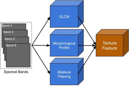
Table 1. Combination of texture features of Sentinel-2.

S. No.	Features	Combination Operation
1	S + B	Concatenate (S, B)
2	S + G	Concatenate (S, G)
3	S + M	Concatenate (S, M)
4	B + G	Concatenate (B, G)
5	B + M	Concatenate (B, M)
6	G + M	Concatenate (G, M)
7	S + B+G	Concatenate (S, B, G)
8	S + B+M	Concatenate (S, B, M)
9	S + G+M	Concatenate (S, G, M)
10	B + G+M	Concatenate (B, G, M)
11	S + B+G + M	Concatenate (S, B, G, M)

Here, S: Spectral; B: Bilateral Filtering; G: GLCM, and M: Morphological profile analysis.

2.3.2. Deep feature extraction

Recent research in the field of remote sensing suggests that deep classifiers can detect distinct patterns that can help in detecting cloudy and non-cloudy regions. In this study, Resnet-based CNN is used to extract low to high-level CNN features (deep features). In Figure 2, Four spectral bands, including Band 4 (Red), Band 3 (Green), Band 2 (Blue), and Band 8 (NIR), are used as input to Resnet, in which two residual blocks are used to perform skip connections over some layer and extract 288 deep features. Two residual blocks used with Resnet are the convolution block that changes the shape of input and the identity block that allows keeping the same input shape. In Resnet, the 2D convolution layer uses a kernel (also known as a filter) to slide over 2D input data to produce new 2D output. Batch normalization regulates the output of the convolution layer by normalizing unstable gradients for the next activation layer, which uses Rectified Linear Unit (ReLU) activation function to transform the received input. Average pooling is used to down sample feature maps, and flattening helped convert the multidimensional output of average pooling to be fed to the used classifiers. To reduce the computational costs, an image patch size of 5 × 5 and Resnet with two convolution blocks and two identity blocks with a total parameter of 152320, including 151296 trainable parameters and 1024 non-trainable parameters, were used (Table 2).

Figure 2. Process of deep feature extraction.

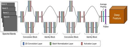
Table 2. Setup of considered Residual Network (Resnet).

Layer/Block	Output	Connected to
Input Layer	(None, 5, 5, 4)	[ ]
Convolution 2D	(None, 5, 5, 64)	Input Layer
Batch_Normalization	(None, 5, 5, 64)	Convolution 2D
Activation	(None, 5, 5, 64)	Batch_Normalization
Convolution Block	(None, 5, 5, 32)	Activation
Identity Block	(None, 5, 5, 32)	Convolution Block
Convolution Block	(None, 5, 5, 32)	Identity Block
Identity Block	(None, 5, 5, 32)	Convolution Block
Average Pooling	(None, 3, 3, 32)	Identity Block
Flatten	(None, 288)	Average Pooling

3. Dataset

In this work, the Baetens-Hagolle Sentinel-2 dataset (Baetens et al. 2019) includes 31 reference L1C images acquired by Sentinel-2 from 10 different sites worldwide, along with seven images from the Holstein dataset (Hollstein et al. 2016) is used. This dataset consists of a manually labeled cloud mask of 60 m spatial pixel resolution for each image, which is used as a reference to evaluate the performance of cloud detection methods. The manual cloud mask of this dataset consists of 7 classes that are labeled from 0 to 7, as displayed in Table 3.

Table 3. Manual Cloud Mask Description of Baetens-Hagolle Sentinel-2 dataset.

Label	Class Name	Label	Class Name
0	No Fill	4	Cloud Shadow
1	No Data	5	Ground
2	Low Cloud	6	Water
3	High Cloud	7	Snow

All images of this dataset are downloaded separately from Copernicus Open Access Hub (European Space Agency (ESA) 2022) and USGS Earth Explorer (U.S. Geological Survey (USGS) 2022). Table 4 provides a brief description of spectral band information of the images acquired by Sentinel-2. Band 4 (Red), Band 3 (Green), Band 2 (Blue), and Band 8 (NIR) are found to have most of the information to perform cloud detection (Xu et al. 2019; Segal-Rozenhaimer et al. 2020), were used in this study. Only these bands were used to derive different textures and deep features for cloud detection throughout.

Table 4. Spectral Band Information of Sentinel 2.

S. No.	Band Name	Band Index	Resolution (meter)	Wavelength (µ-meter)
1	Coastal	Band 1	60	0.433–0.453
2	Blue	Band 2	10	0.458–0.523
3	Green	Band 3	10	0.543–0.578
4	Red	Band 4	10	0.650–0.680
5	Red Edge 1	Band 5	20	0.698–0.713
6	Red Edge 2	Band 6	20	0.733–0.748
7	Red Edge 3	Band 7	20	0.765–0.785
8	Wide NIR	Band 8	10	0.785–0.900
9	Narrow NIR	Band 8A	20	0.855–0.875
10	Water Vapor	Band 9	60	0.930–0.950
11	Cirrus	Band 10	60	1.365–1.385
12	SWIR1	Band 11	20	1.565–1.655
13	SWIR2	Band 12	20	2.100–2.280

Here, NIR is Near Infrared, and SWIR is Shortwave Infrared

Another Sentinel-2 cloud detection dataset named WHUS2-CD is also considered for this study. This includes 32 single-date images of 32 different sites over the mainland China region, where most of the selected images have cloud cover of less than 20% (Li et al. 2021). Labeled reference mask consists of only two classes named Clear and Cloud, where pixels consisting of any cloud type are labeled as a cloud while pixels consisting of ground, snow, water, and cloud shadow are considered as clear. The focus of this dataset is to perform pixel-wise cloud detection as a binary classification problem that separates pixels into two classes (i.e. cloud and clear) for Sentinel-2 imagery.

4. Cloud detection process

Prior to cloud detection, preprocessing of remote sensing images is required as atmospheric scattering contaminates surface reflectance, and dark objects like water are affected by this. In order to determine true surface characteristics, Atmospheric correction using Dark Object Subtraction (DOS1) is used and applied to all images used in this study (Moran et al. 1992).

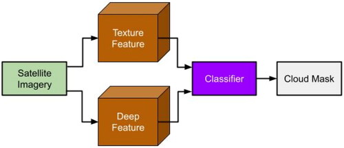
The cloud detection process of generating a cloud mask used in this study is illustrated in Figure 3. A combination of spectral and texture and deep features extracted from satellite imagery were used to train machine learning classifiers (XGBoost, RF, and SVM). These trained classifiers perform pixel-wise classification into six classes: low cloud, high cloud, cloud shadow, ground, snow, and water, and these classes are stored as a cloud mask. This cloud mask helps in locating cloud-affected and cloud-free regions for improved analysis.

Figure 3. Process of cloud detection (mask).

$\mathit{Algorithm}: \mathit{Cloud}\hspace{0.17em}\mathit{Detection}\mathit{\text{\hspace{0.17em}of\hspace{0.17em}}}\mathit{satellite}\hspace{0.17em}\mathit{imagery}\hspace{0.17em}\mathit{for}\hspace{0.17em}\mathit{Sentinel}-2.$

$\mathit{Input}:\hspace{0.17em}S=\mathit{Spectral}\hspace{0.17em}\mathit{band}\hspace{0.17em}\mathit{data}\mathit{\text{ of }}\mathit{image};\mathit{Band}=\left\{\mathit{Red},\mathrm{ }\mathit{Blue},\mathrm{ }\mathit{Green},\mathrm{ }\mathit{NIR}\right\},\hspace{0.17em}\mathit{Pixe}{l}_{\mathit{Resolution}}=60$

$\mathit{Begin}$

$\mathit{Feature}\mathit{ }\mathit{Extraction}:$

  $To\hspace{0.17em}\mathit{select}\hspace{0.17em}\mathit{type}\mathit{\text{\hspace{0.17em}of\hspace{0.17em}}}\mathit{feature}\hspace{0.17em}\mathit{extraction}:$

    $\mathit{If}\hspace{0.17em}(\mathit{feature}==\hspace{0.17em}\mathit{Texture}\hspace{0.17em}||\hspace{0.17em}\mathit{feature}==\hspace{0.17em}\mathit{Deep})$

     $\hspace{0.17em}\mathit{Texture}\leftarrow \mathit{select}(\mathit{GLCM},\hspace{0.17em}\mathit{Morphological},\hspace{0.17em}\mathit{Bilateral})$

    $\mathit{Else}\hspace{0.17em}$

     $\hspace{0.17em}\mathit{Deep}\leftarrow \mathit{ResNet}$

    $\mathit{End} \mathit{if}$

  $To\hspace{0.17em}\mathit{select}\hspace{0.17em}\mathit{Texture}\hspace{0.17em}\mathit{feature}\hspace{0.17em}\mathit{extraction}:$

    $\mathit{select}(\mathit{feature}==\hspace{0.17em}\mathit{GLCM}||\hspace{0.17em}\mathit{feature}==\hspace{0.17em}\mathit{Morpholocial}\hspace{0.17em}||\hspace{0.17em}\mathit{feature}==\hspace{0.17em}\mathit{Bilateral})$

     // For GLCM Features:

     $\hspace{0.17em}G\leftarrow \mathit{GLCM}\left(S,\hspace{0.17em}\mathit{Patc}{h}_{\mathit{Size}}=5,\hspace{0.17em}\mathit{Band}\right)$

      // For Morphological Profiling Features:

     $\hspace{0.17em}M\leftarrow \mathit{Concatenate}(\mathit{opening}(S,\hspace{0.17em}\mathit{Patc}{h}_{\mathit{Size}}=5,\hspace{0.17em}\mathit{Band}),\hspace{0.17em}\mathit{closing}(S,\hspace{0.17em}\mathit{Patc}{h}_{\mathit{Size}}=5,\hspace{0.17em}\mathit{Band}))$

     // For Bilateral Filtering Features:

     $\hspace{0.17em}B\leftarrow \mathit{Bilateral}\left(S,\hspace{0.17em}\mathit{Patc}{h}_{\mathit{Size}}=5,\hspace{0.17em}\mathit{Band}\right)$

$\mathit{Cloud}\mathrm{\hspace{0.17em}\hspace{0.17em}}\mathit{Detection}:$

  $\mathit{Classify}\mathit{ }(\mathit{feature}==\hspace{0.17em}\mathit{Texture}\hspace{0.17em}||\hspace{0.17em}\mathit{feature}==\hspace{0.17em}\mathit{Deep})$

     // For Texture Feature:

     $\mathit{ }\mathit{If}(\mathit{feature}\hspace{0.17em}\mathit{set}==S\hspace{0.17em}||\mathit{feature}\hspace{0.17em}\mathit{set}==B\hspace{0.17em}||\mathit{feature}\hspace{0.17em}\mathit{set}==G\hspace{0.17em}||\mathit{feature}\hspace{0.17em}\mathit{set}==M$

       $\hspace{0.17em}\left|\right|\mathit{feature}\hspace{0.17em}\mathit{set}==S+B\hspace{0.17em}\left|\right|\mathit{feature}\hspace{0.17em}\mathit{set}==S+G\hspace{0.17em}\left|\right|\mathit{feature}\hspace{0.17em}\mathit{set}==S+M$

       $\hspace{0.17em}\left|\right|\mathit{feature}\hspace{0.17em}\mathit{set}==B+M\hspace{0.17em}\left|\right|\mathit{feature}\hspace{0.17em}\mathit{set}==B+G\hspace{0.17em}\left|\right|\mathit{feature}\hspace{0.17em}\mathit{set}==G+M\hspace{0.17em}$

       $\hspace{0.17em}\left|\right|\mathit{feature}\hspace{0.17em}\mathit{set}==S+B+G\hspace{0.17em}\left|\right|\mathit{feature}\hspace{0.17em}\mathit{set}==S+B+M\hspace{0.17em}\left|\right|\mathit{feature}\hspace{0.17em}\mathit{set}==S+G+M$

       $\hspace{0.17em}\left|\right|\mathit{feature}\hspace{0.17em}\mathit{set}==S+B+G\hspace{0.17em}\left|\right|\mathit{feature}\hspace{0.17em}\mathit{set}==S+B+G+M)$

                 $\hspace{0.17em}\mathit{feature}\leftarrow \hspace{0.17em}\mathit{feature}\hspace{0.17em}\mathit{set}$

       $\hspace{0.17em}//\hspace{0.17em}\mathit{For}\hspace{0.17em}\mathit{deep}\hspace{0.17em}\mathit{Features}:$

       $\hspace{0.17em}\mathit{Else}\hspace{0.17em}$

                 $\hspace{0.17em}\mathit{feature}\leftarrow \hspace{0.17em}\mathit{Deep}\hspace{0.17em}$

       $\mathit{End} \mathit{if}$

  $\mathit{clou}{d}_{\mathit{mask}}=\mathit{RandomForest}\left(\mathit{feature}\right)$

  $\mathit{clou}{d}_{\mathit{mask}}=\mathit{SVM}\left(\mathit{feature}\right)$

  $\mathit{clou}{d}_{\mathit{mask}}=\mathit{XGBoost}\left(\mathit{feature}\right)$

  $\mathit{Return}\hspace{0.17em}\mathit{clou}{d}_{\mathit{mask}}$

$\mathit{End}$

$\mathit{Output}\mathit{ }=\hspace{0.17em}\mathit{Generated}\hspace{0.17em}\mathit{cloud}\hspace{0.17em}\mathit{mask}\hspace{0.17em}\mathit{composed}\mathit{\text{ of }}6\hspace{0.17em}\mathit{classes}.$

       {Low Cloud, High Cloud, Cloud Shadow, Ground, Snow, Water}

5. Results and discussion

To evaluate the performance of different machine learning cloud detection methods (XGBoost, RF, and SVM) using the Baetens-Hagolle dataset and WHUS2-CD dataset, various performance measures, including User Accuracy (UA), Producer Accuracy (PA), Overall Accuracy, Kappa coefficient, and F1 score, were used (Tables 6–10). Computational cost and size of classifiers with used datasets are also reported in Table 7. Classified images representing the visual assessment of cloud masks using various cloud detection methods are also provided in Figures 7–24. For computations, a high-performance computing system with Intel(R) Xeon(R) Gold 6132 CPU @ 2.60 GHz having RAM of 96 GB and 16 GB Nvidia graphic card was used.

Table 6. Results of XGBoost, RF and SVM classifiers using Baetens-Hagolle dataset. The best input feature combination is highlighted for all three classifiers.

S. No	Features	Accuracy (%)			Kappa
		XGBoost	RF	SVM	XGBoost	RF	SVM
1	S	85.8	86.1	78.5	0.665	0.678	0.437
2	B	87.5	88.6	79.5	0.710	0.741	0.469
3	G	80.3	80.1	79.7	0.451	0.446	0.434
4	M	89.0	90.8	82.6	0.746	0.807	0.561
5	S + B	88.1	89.9	79.6	0.723	0.770	0.470
6	S + G	87.7	87.7	83.3	0.711	0.714	0.573
7	S + M	89.7	94.1	82.9	0.766	0.862	0.569
8	B + G	88.9	89.6	83.9	0.744	0.763	0.593
9	B + M	90.3	93.1	83.2	0.779	0.860	0.577
10	G + M	89.4	92.6	84.1	0.757	0.832	0.598
11	S + B+G	89.1	90.1	84.0	0.749	0.772	0.596
12	S + B+M	90.3	94.2	83.2	0.780	0.870	0.578
13	S + G+M	90.0	92.3	84.4	0.771	0.825	0.610
14	B + G+M	90.4	93.4	84.4	0.783	0.850	0.614
15	S + B+G + M	90.5	92.8	84.9	0.784	0.836	0.624

Table 7. Numerical results of considered cloud detection methods for Baetens-Hagolle dataset.

Metrics		XGBoost		RF		SVM
		S + B+G + M	Deep	S + B+M	Deep	S + B+G + M	Deep
UA (%)	Low Cloud	77.7	80.2	86.8	82.4	60.3	75.4
	High Cloud	57.7	65.5	76.6	66.8	37.3	56.9
	Cloud Shadow	63.9	63.6	72.5	61.7	9.8	53.1
	Ground	98.3	98	98.9	98.6	99.3	98.4
	Water	88.2	89.1	90.8	87.9	74.1	84.2
	Snow	72.1	64.4	74.2	56.3	28	54.7
PA (%)	Low Cloud	77.1	80.6	87.6	82.6	70.1	77.4
	High Cloud	77.3	78.5	89.9	83.4	68.7	74.7
	Cloud Shadow	77.1	75	85.4	81.3	64.3	72.2
	Ground	94.6	95.2	96.2	95	88.4	93.8
	Water	92.9	91.5	95.6	94.2	76	90.8
	Snow	85.6	82.8	91.5	91.5	82.7	84.4
Accuracy (%)		90.5	91.3	94.2	92.1	84.9	89.7
Kappa		0.784	0.80	0.87	0.82	0.62	0.76
Prediction Time (sec)		23.28	34.24	176.58	1540.98	2148.96	9129.65
Size of Classifier (kb)		4,871	5,007	13,966,954	12,372,374	10	36

Table 8. Conversion of multiple classes to binary classes for cloud detection.

Binary Class	Machine Learning Based		Fmask		Sen2Cor
	Label	Class	Label	Class	Label	Class
Contaminated	2 3 4	Low cloud High cloud Cloud shadow	2 4	Cloud shadow Cloud	3 8 9 10	Cloud shadows Cloud medium probability Cloud high probability thin cirrus
Clear	5 6 7	Ground Water Snow	0 1 3	Clear land Water Snow	2 4 5 6 7 11	Dark area pixels Vegetation Bare soils Water Unclassified snow

Table 9. Numerical results of considered cloud detection methods for Baetens-Hagolle dataset.

Classifier		Metrics	Railroad Valley (USA)	Alta Floresta (Brazil)	Alta Floresta (Brazil)	Marrakech (Morocco)	Arles (France)	Orleans (France)	Ispra (Italy)	Gobabeb (Namibia)	Mongu (Zambia)	Pretoria (South Africa)	Munich (Germany)	Munich (Germany)	Average
XGBoost	S + B+G + M	Accuracy	91.4	96.8	90	83.8	88.9	93.3	90.9	86.2	94.3	92	97.1	88.2	91.1
		F1 Score	92.5	49.2	70.6	73.9	92.7	74.4	41.6	79.5	71.8	78.2	61.2	91.5	73.1
	Deep	Accuracy	92	96.7	88.7	83.1	90	90.2	92	83	92.4	88.8	96.5	88.1	90.1
		F1 Score	93.1	50.5	68.7	73.5	93.5	67.6	53.4	75.6	66.6	73.6	55.2	91.4	71.9
RF	S + B+M	Accuracy	91.6	96.7	89.9	84.2	88.7	92.8	91.1	85.5	94.3	91.3	96.9	88.5	90.9
		F1 Score	92.8	47	71.3	75	92.5	73.3	46.7	78.8	71.8	76.6	58.4	91.7	73
	Deep	Accuracy	92.4	96.8	89.6	82.6	90.4	91.9	91.3	83.4	93	90.6	97.3	88.1	90.6
		F1 Score	93.4	48.1	70.2	71.4	93.7	71.8	48.9	76	67.2	75.3	61	91.3	72.3
SVM	S + B+G + M	Accuracy	90.2	95.4	88.2	71.1	91.9	81.4	89.2	80.5	92.1	89.7	96.6	63.4	85.8
		F1 Score	91.6	28.8	63.3	40.5	94.6	53.4	13.2	73.4	60.3	72.9	48.9	67.8	59.1
	Deep	Accuracy	91.7	97	89.1	82.6	90.4	92.5	91.3	83.8	94.4	90.8	97	87.2	90.7
		F1 Score	92.7	49.5	67.1	70.6	93.7	73	44.1	76.8	71.4	74.6	60.1	90.6	72
Fmask [54]		Accuracy	89.5	97.4	78.8	89.1	95.1	94.4	91.7	91.9	76.3	97.1	98	88.8	90.7
		F1 Score	91.2	63.3	61.4	70.2	80.2	96.3	86.1	47.3	70.2	88.2	69.5	92.3	76.3
Sen2cor [54]		Accuracy	80.1	95.9	89.2	87.9	91.8	78.5	85.9	93	89.6	97	98.2	85.1	89.4
		F1 Score	82	15.2	83.3	51.8	61.8	84.1	75.1	56.9	89.2	85.7	67	89	70.1
MAJA [54]		Accuracy	89.9	97.1	90	93.7	95.2	93.8	89.3	94.6	85.7	96.4	97.8	91.6	92.9
		F1 Score	91.6	60	84.9	81.7	80.2	95.9	82.4	71	84	82.8	63.2	94.4	81

Table 10. Numerical results of considered cloud detection methods for WHUS2-CD dataset.

Metrics	XGBoost		RF		SVM		Resnet	CDFM3SF-4 (Li et al. 2021)	Fmask	Sen2Cor
	Texture	Deep	Texture	Deep	Texture	Deep
UA%	74.16	84.29	76.16	83.18	56.07	83.97	84.69	82.50	59.90	64.20
PA%	78.03	88.27	80.07	89.78	79.40	87.91	87.22	97.91	95.14	69.36
Accuracy (%)	96.41	98.11	97.16	98.23	95.23	98.13	98.00	98.68	92.62	90.89

5.1. Results of Baetens-Hagolle dataset

The results of cloud detection for the Baetens-Hagolle dataset are evaluated in three phases. In the first phase, 18 images from 9 sites are selected, as displayed in Table 5, to train and locally test machine learning classifiers by dividing the total data in a way to use 25% for training and the rest for testing. In the second phase, trained classifiers are tested with the remaining 12 images of the Baetens-Hagolle dataset to assess the generalization capabilities of various classifiers as well as for visual assessment. Finally, a comparison of considered classifiers is carried out with state-of-the-art threshold-based methods (i.e. Fmask, Sen2cor, MAJA) by using test imagery of the second phase, which consists of a variety of clouds and ground information in different percentages.

Table 5. Description of Baetens-Hagolle Sentinel-2 dataset.

	Scene ID	Scene information
Phase 1	S2A_MSIL1C_20170501T183311_N0205_R127_T11SPC_20170501T183311	Small cumulus over bright soil
	S2B_MSIL1C_20170827T182909_N0205_R027_T11SPC_20170827T183954	Large cumulus over bright soil
	S2A_MSIL1C_20180505T141051_N0206_R110_T21LWK_20180505T160911	Scattered small cumulus
	S2B_MSIL1C_20180609T141049_N0206_R110_T21LWK_20180609T173247	Thin cirrus
	S2A_MSIL1C_20160417T110652_N0201_R137_T29RPQ_20160417T111159	Scattered cumulus and thin cirrus
	S2A_MSIL1C_20170621T110651_N0205_R137_T29RPQ_20170621T111222	Clear image with snow and thin cirrus
	S2A_MSIL1C_20170917T103021_N0205_R108_T31TFJ_20170917T103018	Large cloud cover
	S2B_MSIL1C_20171002T103009_N0205_R108_T31TFJ_20171002T103209	Thick and thin clouds
	S2A_MSIL1C_20170516T105031_N0205_R051_T31UDP_20170516T105322	Thick and thin cirrus clouds
	S2B_MSIL1C_20170819T105029_N0205_R051_T31UDP_20170819T105403	Large mid-altitude cloud cover
	S2A_MSIL1C_20170815T102021_N0205_R065_T32TMR_20170815T102513	Clouds over mountains with snow
	S2B_MSIL1C_20171009T102009_N0205_R065_T32TMR_20171009T102008	Clouds over mountains with snow and bright soil
	S2A_MSIL1C_20161221T085352_N0204_R107_T33KWP_20161221T091140	Thick clouds above the desert
	S2B_MSIL1C_20170909T084009_N0205_R064_T33KWP_20170909T090455	Small and low clouds
	S2A_MSIL1C_20161112T082202_N0204_R121_T34LGJ_20161112T083553	Large thick cloud cover and some cirrus
	S2B_MSIL1C_20170804T081559_N0205_R121_T34LGJ_20170804T083419	Clear image and a few mid-altitude clouds
	S2A_MSIL1C_20170313T074931_N0204_R135_T35JPM_20170313T081339	Diverse cloud types
	S2A_MSIL1C_20170820T074941_N0205_R135_T35JPM_20170820T081632	Scattered small clouds
Phase 2	S2B_MSIL1C_20180213T183449_N0206_R027_T11SPC_20180213T214845	Large stratus and some cumulus
	S2A_MSIL1C_20180714T141051_N0206_R110_T21LWK_20180714T155753	Mid-altitude small clouds
	S2A_MSIL1C_20180813T141051_N0206_R110_T21LWK_20180813T174352	Thin cirrus
	S2A_MSIL1C_20171218T111451_N0206_R137_T29RPQ_20171218T132926	Scattered cumulus and snow
	S2B_MSIL1C_20171221T103429_N0206_R108_T31TFJ_20171221T123944	Mid-altitude thick clouds and snow
	S2B_MSIL1C_20180218T110109_N0206_R094_T31UDP_20180218T162525	Stratus cloud
	S2B_MSIL1C_20171111T103239_N0206_R108_T32TMR_20171111T124420	Clouds over mountains and mist
	S2B_MSIL1C_20180209T085109_N0206_R107_T33KWP_20180209T123639	High and thin clouds
	S2B_MSIL1C_20171013T081959_N0205_R121_T34LGJ_20171013T083556	Large thin cirrus cover
	S2B_MSIL1C_20171213T075319_N0206_R135_T35JPM_20171213T112619	Altostratus and small scattered clouds
	S2A_MSIL1C_20180422T102031_N0206_R065_T32UPU_20180422T141352	Mostly cloud-free with a few small clouds
	S2B_MSIL1C_20180424T101029_N0206_R022_T32UPU_20180424T124227	Large cloud cover with cumulus and cirrus

5.1.1. First phase

Table 6 reports the accuracy and kappa value of considered machine learning methods (XGBoost, RF, and SVM) using a combination of 15 texture features where the best input feature combination is highlighted. RF achieved highest accuracy of 94.2% (Kappa value = 0.870) with S + B+M features in comparison to XGBoost and SVM classifiers having classification accuracy of 90.5% and 84.9% (Kappa value = 0.771, 0.624) respectively using S + B+G + M features respectively. Individual features such as S, B, G, and M performed poorly with all three classifiers. Combining spectral information with textural information improved detection accuracy compared to the results with spectral information alone.

Table 7 provides results with the Baetens-Hagolle dataset using both traditional as well as deep features using XGBoost, RF, and SVM classifiers. Results indicate that low cloud pixels are commonly considered thick clouds, high clouds are commonly considered thin clouds, and cloud shadow is better identified by RF classifier using S + B+M texture features. It outperformed XGBoost and SVM by achieving the highest Overall Accuracy as well as User Accuracy (UA) and Producer Accuracy (PA) of each class, except for UA of the ground class. SVM with S + B+G + M for the ground area is better than other considered machine learning methods, but it confuses snow as cloud and cloud shadow as water.

Results (Table 7) also suggest inferior performance by Resnet-based deep features in comparison to the traditional texture features with RF and XGBoost-based methods. A possible reason for poor performance using deep features may be due to the misclassification of snow with cloud and terrain shadow with cloud shadow. Additional parameters like prediction time and size of classifiers are also taken into consideration to compare the speed and cost of computation. XGBoost-based cloud detection methods take about 1/10 the time, and the size of the classifier is 2000 times smaller than RF classifier.

5.1.2. Second phase

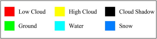
To visually assess and bring out the visual comparative analysis of traditional texture and deep feature-based cloud detection, each class of generated cloud masks is color-coded, as in Figure 4.

Figure 4. Color code for cloud mask.

Figure 5(a) displays a true color image of railroad valley (USA) tile 11SPC dated 13/02/2018, having large stratus and cumulus high cloud region over bright soil and mountainy region. Figure 5(b) is a color-coded manual mask, whereas Figure 5(c)–(h) is a color-coded cloud mask generated by considered cloud detection methods. The comparison of cloud masks suggests that all machine learning methods used in this study confused low cloud with high cloud due to the high brightness and thickness of the cloud, but the overall contamination detection rate is quite good. Deep features showed better cloud shadow detection with all three classifiers (Figure 5) in comparison to traditional texture-based features.

Figure 5. Railroad Valley (USA) (a) True Color image, (b) Manual reference mask, generated cloud mask by: (c) RF with traditional texture features (d) RF with deep features (e) XGBoost with traditional texture features (f) XGBoost with deep features, (g) SVM with traditional texture features, and (h) SVM with deep features.

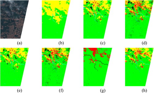
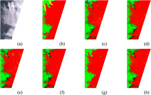
Figures 6(a) and 7(a) consists of a true color image acquired over the equatorial forest region with tile id 21LWK (dated 14/07/2018 and 13/08/2018), having the small cloud of medium altitude labeled as low and thin cirrus cloud, respectively. Figures 6(b) and 7(b) is color-coded manual mask whereas Figures 6(c)–(h) and 7(c)–(h) is color-coded cloud mask generated by considered cloud detection methods. XGBoost classifier (Figures 6(e,f) and 7(e,f)) performed better than other considered methods for this dataset. Thin clouds, commonly considered as high clouds, with very high opacity, were identified as cloud-free by considered classifiers because preprocessing performs subtraction operation of the dark area, which end up correcting those blurred thin cloudy pixels, and high cloud is often included in the manual mask from band 10 of Sentinel 2. Better detection of water region is notable with XGBoost classifier In Figures 6(e,f) and 7(e,f). SVM is found to misclassify rivers as cloud shadows when used with traditional texture features (Figure 6(g) and 7(g)). Deep features-based cloud detection (Figures 6(h) and 7(h)) performed well with this dataset.

Figure 6. Alta Floresta (Brazil) (a) True Color image, (b) Manual reference mask, generated cloud mask by: (c) RF with traditional texture features (d) RF with deep features (e) XGBoost with traditional texture features (f) XGBoost with deep features, (g) SVM with traditional texture features, and (h) SVM with deep features.

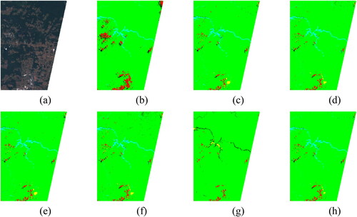
Figure 7. Alta Floresta (Brazil) (a) True Color image, (b) Manual reference mask, generated cloud mask by: (c) RF with traditional texture features (d) RF with deep features (e) XGBoost with traditional texture features (f) XGBoost with deep features, (g) SVM with traditional texture features, and (h) SVM with deep features.

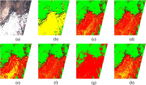
Figure 8(a) displays a true color image acquired over Marrakech (Morocco, tile 29RPQ dated 18/12/2017), having a mountainous region with surface elevation varying from 450 to 4000 m above sea level. The scene has snow on the mountain peak and scattered low cumulus clouds in the lower region. Figure 8(b) is a color-coded manual mask, and Figure 8(c)–(h) is a color-coded cloud mask generated by considered cloud detection methods. The detection rate of cloud vs. snow is better with considered methods except for SVM with traditional textures (Figure 8). Mismatch of terrain shadow as cloud shadow is detected accurately by XGBoost using traditional texture features (Figure 8(e)).

Figure 8. Marrakech (Morocco) (a) True Color image, (b) Manual reference mask, generated cloud mask by: (c) RF with traditional texture features (d) RF with deep features (e) XGBoost with traditional texture features (f) XGBoost with deep features, (g) SVM with traditional texture features, and (h) SVM with deep features.

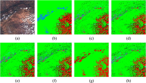
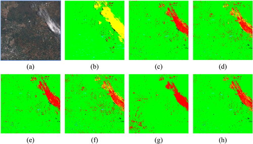
Figure 9(a) represents true color imagery from Arles (France, tile 31TFJ dated 21/12/2017), having the sea with the mountain region having the thick middle-level cloud labeled as the low cloud. Figure 9(b) is a color-coded manual mask and Figure 10(c)–(h) is a color-coded cloud mask generated by considered cloud detection methods. XGBoost with traditional texture features (Figure 9(h)) achieved the best results with this dataset. This approach was able to better handle the confusion of cloud and snow to some extent over the ground, but a small portion of cloud over the sea region is misclassified as snowy. All classifiers, when used with deep features (Figures 10(d), (f) and (h)), were able to handle snow-cloud confusion well over the sea region.

Figure 9. Arles (France) (a) True Color image, (b) Manual reference mask, generated cloud mask by: (c) RF with traditional texture features (d) RF with deep features (e) XGBoost with traditional texture features (f) XGBoost with deep features, (g) SVM with traditional texture features, and (h) SVM with deep features.

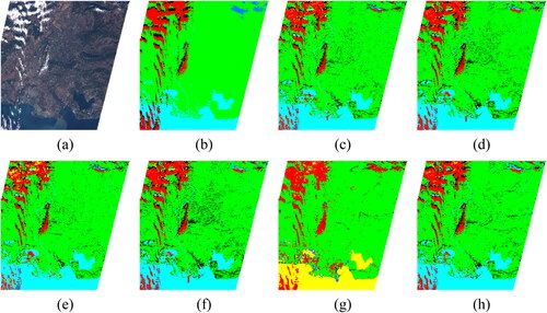
Figure 10. Orleans (France) (a) True Color image, (b)Manual reference mask, generated cloud mask by: (c) RF with traditional texture features (d) RF with deep features (e) XGBoost with traditional texture features (f) XGBoost with deep features, (g) SVM with traditional texture features, and (h) SVM with deep features.

Figure 10(a) displays true color imagery from Orleans (France, tile 31UDP dated 18/02/2018), having a large stratus cloud over the flat agricultural site. Figure 10(b) is a color-coded manual mask, and Figure 10(c)–(h) is a color-coded cloud mask generated by considered cloud detection methods. Considered classifiers with both traditional and deep features detected thick cloud portion accurately while high cloud is marked as a low cloud in some portion. The dark field area, which is misjudged as cloud shadow by other classifiers (Figure 11(c)–(f) and (h)), is handled well by SVM with traditional texture features (Figure 10(g)).

Figure 11. Ispra (Italy) (a) True Color image, (b) Manual reference mask, generated cloud mask by: (c) RF with traditional texture features (d) RF with deep features (e) XGBoost with traditional texture features (f) XGBoost with deep features, (g) SVM with traditional texture features, and (h) SVM with deep features.

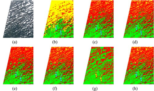
Figure 11(a) provides true color imagery from Ispra (Italy; tile 32TMR dated 11/11/2017), comprising rich diversity and thick clouds over the snow region marked as low clouds. Figure 11(b) is a color-coded manual mask, whereas Figure 11(c)–(h) is a color-coded cloud mask generated by the considered cloud detection method. It can be seen from Figure 11(a) and (b) that considered machine learning classifiers achieve good performance except SVM with traditional texture features (Figure 11(g)) for overall cloud detection. On the other hand, XGBoost with traditional texture features (Figure 11(e)) achieves the best cloud shadow detection result.

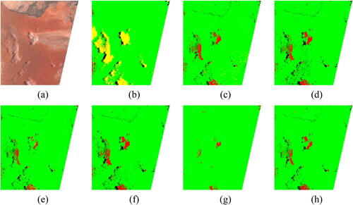
Figure 12(a) represents true color imagery from the desert site of Gobabeb (Namibia, tile-id 33KWP dated 09/02/2018) with thin cloud and cloud shadow. Figure 12(b) is a color-coded manual mask, whereas Figure 12(c)–(h) is a color-coded cloud mask generated by considered cloud detection methods. With deep features, only thin cloud with high opacity is detected as cloud and cloud shadow detection using XGboost and RF (Figure 12(d) and (f)). The use of deep features brings out enhanced details in comparison to traditional texture features for the desert area while confusion of high cloud as low cloud persists.

Figure 12. Gobabeb (Namibia) (a) True Color image, (b) Manual reference mask, generated cloud mask by: (c) RF with traditional texture features (d) RF with deep features (e) XGBoost with traditional texture features (f) XGBoost with deep features, (g) SVM with traditional texture features, and (h) SVM with deep features.

Figures 13(a) and 14(a) display true color imagery with the thin cloud over grassland, savannah, and dry woodland from two different locations (Mongu (Zambia) tile 34LGJ dated 13/10/2017 and Pretoria (South Africa) tile 35JPM dated 13/12/2017) respectively. Figures 13(b) and 14(b) is color-coded manual mask whereas Figures 13(c)–(h) and 14(c)–(h) is color-coded cloud mask generated by considered cloud detection methods. XGBoost with traditional texture features (Figures 13(e) and 14(e)) performed better in detecting cloud and cloud shadow more accurately than RF and SVM. The high cloud is mismatched with the low cloud because of high opacity, which is clearly visible in the true color image (Figures 13(a) and 14(a)), but the overall detection rate is the same for both images. Deep feature based classification (Figures 13 and 14(d), (f) and (h)) performed better than traditional texture feature based classification (Figures 13 and 14(c), (e) and (g)).

Figure 13. Mongu (Zambia) (a) True Color image, (b) Manual reference mask, generated cloud mask by: (c) RF with traditional texture features (d) RF with deep features (e) XGBoost with traditional texture features (f) XGBoost with deep features, (g) SVM with traditional texture features, and (h) SVM with deep features.

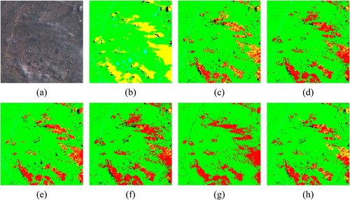
Figure 14. Pretoria (South Africa) (a) True Color image, (b) Manual reference mask, generated cloud mask by: (c) RF with traditional texture features (d) RF with deep features (e) XGBoost with traditional texture features (f) XGBoost with deep features, (g) SVM with traditional texture features, and (h) SVM with deep features.

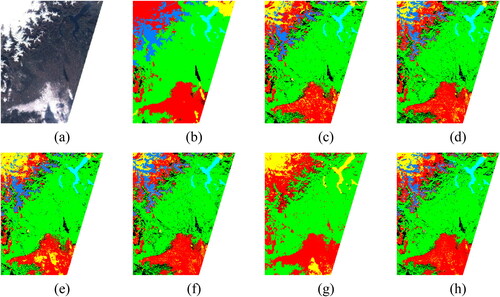
Figures 15(a) and 16(a) provide true color images from Munich (Germany, tile 32UPU, dated 22/04/2018 and 24/04/2018), respectively. Figures 15(b) and 16(b) is color-coded manual mask whereas Figures 15(c)–(h) and 16(c)–(h) is color-coded cloud mask generated by considered cloud detection methods. The imagery of the German site was not used during the training and testing of different algorithms. This was done to evaluate the performance of trained models on an independent site. The image acquired on 22-April has a few small low clouds over agricultural land and small water ponds, as in Figure 15, while the image acquired on 24-April has a large low and high cloud area (Figure 16). RF and XGBoost with traditional texture features detected the contaminated region more accurately (Figures 15(c,e) and 16(c,e), respectively). SVM with traditional texture features (Figures 15(g) and 16(g)) confused water area as high cloud, while deep features displayed in Figures 15(h) and 16(h) show an improved rate of water area detection.

Figure 15. Munich (Germany) (a) True Color image, (b) Manual reference mask, generated cloud mask by: (c) RF with traditional texture features (d) RF with deep features (e) XGBoost with traditional texture features (f) XGBoost with deep features, (g) SVM with traditional texture features, and (h) SVM with deep features.

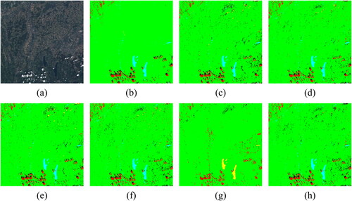
Figure 16. Munich (Germany) (a) True Color image, (b) Manual reference mask, generated cloud mask by: (c) RF with traditional texture features (d) RF with deep features (e) XGBoost with traditional texture features (f) XGBoost with deep features, (g) SVM with traditional texture features, and (h) SVM with deep features.

5.1.3. Comparison with state-of-the-art methods

Table 8 outlines the conversion mechanism as different cloud detection methods generate cloud masks consisting of multiple classes. To compare the results, these multiple classes are grouped into binary classes. Pixels belonging to cloud and cloud shadow are marked as contaminated, whereas pixels belonging to the ground area, snow, water, or unclassified are marked as clear (Baetens et al. 2019).

Table 9 provide a comparison of machine learning cloud detection methods used in this study with state-of-the-art threshold-based methods in term of accuracy and F1 score by using 12 test images. Results from Table 9 suggest improved performance by machine learning-based methods in comparison to state-of-the-art methods. Results suggest that XGBoost with S + B+G + M features achieves the highest average accuracy of 91.1% and F1 score value of 73.1%. It took less than 2 s to generate a mask for each scene. It even outperformed Sen2Cor and Fmask in terms of accuracy. RF-based cloud detection, which achieved such high accuracy locally with 75% test data, is outperformed by XGBoost-based cloud detection in real-world scenarios globally. Although MAJA seems to be better than XGBoost for some images, but it requires cloud-free information for each pixel prior to detection. Moreover, the cloud-free image should be acquired within 30 days of acquiring a cloudy image, whereas machine learning classifiers do not have such constraints (Baetens et al. 2019; Sanchez et al. 2020).

5.2. Results of WHUS2-CD dataset

The potential of proposed machine learning-based cloud detection methods is also evaluated with the WHUS2-CD dataset consisting of 24 images for training, and the remaining eight images for testing were also used (Li et al. 2021). To reduce the computation work, the best combination of texture features as used in Section 5.1 was used. Thus, for RF classifier with feature combination of S + B+M and XGBoost and SVM with S + B+G + M feature combination was used. Resnet is again used to derive deep features with this dataset also. Comparison of considered methods is carried out with state-of-the-art threshold-based methods including Fmask, Sen2cor along with two lightweight deep learning models including Resnet itself and cloud detection-fusing multiscale spectral and spatial features (CD-FM3SF-4) as proposed by Li et al. (2021). For the used dataset, CD-FM3SF-4 took 4 to 8 days of training time, while Resnet took approximately 3 to 4 days for training (Li et al. 2021).

Table 10 reports the comparison of machine learning methods with state-of-the-art threshold-based cloud detection methods in terms of User Accuracy (UA), Producer Accuracy (PA), and overall Accuracy with the WHUS2-CD dataset. Resnet achieved the highest UA of 84.69%, that is the good detection rate of cloud with comparable accuracy to that achieved by CDFM3SF-4, whereas the PA of CDFM3SF-4 is better than other considered cloud detection methods. Considered machine learning methods showed better performance with deep features over traditional features. RF with deep features achieved the highest PA and overall accuracy than RF with traditional features and XGBoost and SVM with deep as well as traditional features. XGBoost with deep features turned out to be the fastest among different methods, with less than 2 s to generate a mask for each scene and achieved comparable performance. All machine learning-based methods outperformed threshold-based cloud detection, that is Fmask and Sen2cor, while Fmask achieved the second highest PA.

Table 11 reports the results of machine learning cloud detection methods on 8 test images of the WHUS2-CD dataset in terms of Accuracy and F1 score. CD-FM3SF-4 achieved the highest average accuracy of 98.68%, with an average F1 score of 89.40% for cloud detection, while Resnet achieved a comparable result with an accuracy of 98% and an F1 score of 85.36%. RF with deep features exhibited better performance than XGBoost and SVM for binary cloud detection. RF with traditional features also outperformed XGBoost and SVM with traditional features for binary cloud detection. Deep features provided better results for binary cloud detection than traditional features because deep features help in distinguishing objects from the cloud with similar surface reflectance like snow and buildings in binary cloud detection. On the other hand, traditional texture features fail to highlight these characteristics in binary cloud detection because pixels belonging to the snow and building class are fewer than other clear pixels, which leads to the imbalance problem. Traditional texture features exhibited better performance in multiclass classification problems where snow class is separated from clear. A major drawback of binary cloud detection is an additional computation for cloud shadow, which has equal importance as the cloud.

Table 11. Numerical results of considered cloud detection methods for WHUS2-CD dataset.

Methods	Features	Metrics	Zhanjiang	Changzhou and Wuxi	Linshui	Yilan	Baotou	Altay	Tibet	Tibet	Average
XGboost	Texture	Accuracy	99.61	98.74	99.63	92.48	98.63	94.25	94.64	93.31	96.41
		F1 score	74.81	72.13	84.27	91	83.04	51.6	62.33	78.58	74.72
	Deep	Accuracy	99.76	99.04	99.78	95.10	99.09	97.27	98.62	96.26	98.11
		F1 score	84.73	77.71	89.86	94.41	89.79	71.70	88.9	88.9	85.75
RF	Texture	Accuracy	99.63	98.68	99.63	93.65	98.59	93.79	99.59	93.68	97.16
		F1 score	76.1	72.03	76.10	92.58	83.07	49.25	82.6	82.04	76.72
	Deep	Accuracy	99.75	99.06	99.76	95.32	99.08	97.27	98.78	96.78	98.23
		F1 score	84.16	77.27	89.4	94.61	89.49	71.61	90.02	90.15	85.84
SVM	Texture	Accuracy	99.46	98.61	99.32	89.52	98.28	93.69	91.44	91.51	95.23
		F1 score	55.65	57.57	62.76	86.82	77.6	35.28	48.25	74.44	62.30
	Deep	Accuracy	99.74	99.01	99.75	95.16	99.11	97.09	98.54	96.6	98.13
		F1 score	83.94	77.38	89.05	94.41	89.99	70.5	88.22	89.71	85.40
Resnet		Accuracy	99.77	99.10	99.77	95.08	99.12	96.89	98.37	95.9	98.00
		F1 score	85.31	79.13	89.75	94.31	90.11	69.11	87.21	87.94	85.36
CD-FM3SF-4 (Li et al. 2021)		Accuracy	99.76	99.38	99.74	95.87	99.29	99.05	98.92	97.38	98.67
		F1 score	84.71	85.01	88.70	95.23	91.82	87.41	90.78	91.68	89.41

Figures 18(a), 19 (a), and 20(a) display true color imagery of Zhanjiang, Changzhou and Wuxi, and Linshui (China), respectively, having less than 20% scattered small clouds over shrubland, water, and urban land region. Figures 18(b), 19 (b), and 20(b) displays color-coded manual mask, and Figures 18(c–j), 19(c–j), and 20(c–j) are the cloud mask generated by machine learning-based cloud detection methods. All machine learning and deep learning methods achieve very high accuracy for cloud detection (i.e. 99%).

Figure 20(a) represents true color imagery over Yilan (China), having about 65% of cloud cover over the barren and forest regions. Figure 20(b) is a color-coded manual mask, while Figure 20(c–j) is the color-coded mask generated by different machine learning and deep learning cloud detection methods. All methods achieved almost similar cloud detection accuracy during visual interpretation.

Figure 21(a) represents true color imagery over Baotou (China), having about 20% of cloud cover over the barren region. Figure 21(b) is a color-coded manual mask, while Figure 21(c–j) is the color-coded mask generated by different machine learning and deep learning cloud detection methods. Again, all methods achieved almost similar cloud detection, but the results of CDFM3SF-4, as displayed in Figure 21(j), detect slightly less amount of cloud and fail to detect very small cloud present in the bottom right area of imagery.

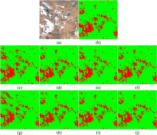
Figure 22(a) displays true color imagery of Altay (China) and Figures 23(a) and 24(a) display true color imagery of the Tibet region, having less than 20% cloud over barren and snow region. Figures 23(b) and 24(b) displays color-coded manual mask, and Figures 23(c)–24(j) displays generated cloud mask by machine learning and deep learning-based cloud detection methods. Machine learning-based cloud detection with traditional texture features is found to misclassify large snow as cloudy, while with deep features, this confusion is better handled to some extent. CDFM3SF-4, as displayed in Figures 23(j) and 24(j), achieve a slightly better result for cloud and snow classification than Resnet and other machine learning methods with deep features, as displayed in Figure 22(i)–24(i) and Figure 22(d, f, h)–24(d, f, h), respectively, as they misclassified innermost pixels of large snow area as the cloud.

5.3. Discussion

The large-scale multispectral data acquired by Sentinel 2A and 2B require fast and accurate cloud detection to recover the distortion caused by the different types of cloud and cloud shadow. Single date threshold-based state-of-the-art cloud detection methods like Fmask and Sen2Cor work on the static threshold where Fmask often include a greater number of cloud pixels based on neighboring cloud pixels, and Sen2Cor often leaves out cloud pixels due to the high spectral reflectance threshold (Table 9). Fmask performance seems much better than Sen2Cor, but multitemporal threshold-based MAJA outperformed both because its thresholds are updated as per cloud-free image of the same location. Machine learning-based cloud detection methods like XGBoost, RF, and SVM using traditional texture features and deep features achieved better performance than Sen2Cor and Fmask for detection of cloud as a multiclass classification problem (Table 9). Machine learning-based cloud detection methods exhibited slightly inferior results than MAJA because features of the different regions of the world are very different, which leads to the misclassification of certain cloudy pixels with the pixel having a similar reflective index. One major problem with MAJA is the requirement of cloud-free imagery, while machine learning-based and other single-date cloud detection have no such requirement. The higher computation cost of deep learning cloud detection methods for creating cloud masks is reduced by lightweight deep learning methods to some extent, but training time is still very high. The lightweight version of Resnet exhibited comparable performance to CDFM3SF-4 for binary cloud detection, and it provides excellent spectral and spatial features (Figures 17–24). CD-FM3SF-4 model is good for binary cloud detection only as its performance degraded for multiclass detection of thin, thick clouds and cloud shadows. The idea of using deep features for machine learning classifiers like XGBoost, RF, and SVM performed well with smaller training and testing time for different regions (Table 7 and Figures 5–24). Deep features extract good quality texture information that perfectly distinguishes clouds from objects with a similar reflective index like snow (Figures 8, 9, 11 and 22), buildings (Figures 10, 13 and 14), and brighter desert areas (Figures 12, 23 and 24).

Figure 17. Zhanjiang (China) (a) True Color image, (b) Manual reference mask, generated cloud mask by: (c) RF with traditional texture features (d) RF with deep features (e) XGBoost with traditional texture features (f) XGBoost with deep features, (g) SVM with traditional texture features, and (h) SVM with deep features, (i) Resnet, and (j) CD-FM3SF-4.

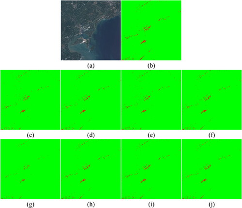
Figure 18. Changzhou and Wuxi (China) (a) True Color image, (b) Manual reference mask, generated cloud mask by: (c) RF with traditional texture features (d) RF with deep features (e) XGBoost with traditional texture features (f) XGBoost with deep features, (g) SVM with traditional texture features, and (h) SVM with deep features, (i) Resnet, and (j) CD-FM3SF-4.

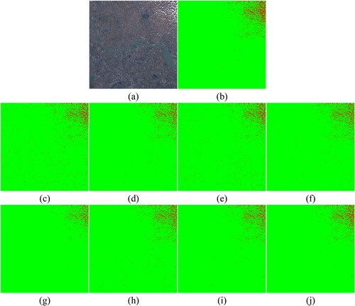
Figure 19. Linshui (China) (a) True Color image, (b) Manual reference mask, generated cloud mask by: (c) RF with traditional texture features (d) RF with deep features (e) XGBoost with traditional texture features (f) XGBoost with deep features, (g) SVM with traditional texture features, and (h) SVM with deep features, (i) Resnet, and (j) CD-FM3SF-4.

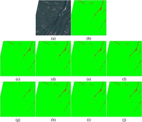
Figure 20. Yilan (China) (a) True Color image, (b) Manual reference mask, generated cloud mask by: (c) RF with traditional texture features (d) RF with deep features (e) XGBoost with traditional texture features (f) XGBoost with deep features, (g) SVM with traditional texture features, and (h) SVM with deep features, (i) Resnet, and (j) CD-FM3SF-4.

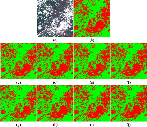
Figure 21. Baotou (China) (a) True Color image, (b) Manual reference mask, generated cloud mask by: (c) RF with traditional texture features (d) RF with deep features (e) XGBoost with traditional texture features (f) XGBoost with deep features, (g) SVM with traditional texture features, and (h) SVM with deep features, (i) Resnet, and (j) CD-FM3SF-4.

Figure 22. Altay (China) (a) True Color image, (b) Manual reference mask, generated cloud mask by: (c) RF with traditional texture features (d) RF with deep features (e) XGBoost with traditional texture features (f) XGBoost with deep features, (g) SVM with traditional texture features, and (h) SVM with deep features, (i) Resnet, and (j) CD-FM3SF-4.

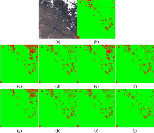
Figure 23. Tibet (a) True Color image, (b) Manual reference mask, generated cloud mask by: (c) RF with traditional texture features (d) RF with deep features (e) XGBoost with traditional texture features (f) XGBoost with deep features, (g) SVM with traditional texture features, and (h) SVM with deep features, (i) Resnet, and (j) CD-FM3SF-4.

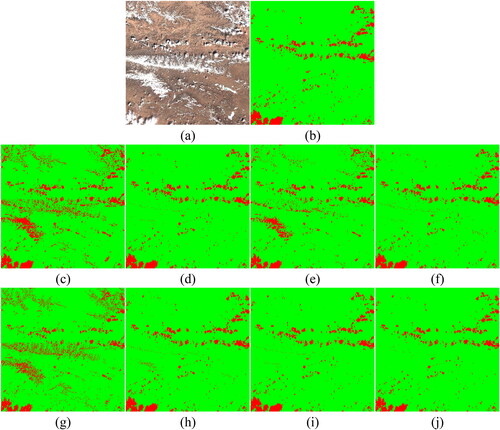
Figure 24. Tibet (a) True Color image, (b) Manual reference mask, generated cloud mask by: (c) RF with traditional texture features (d) RF with deep features (e) XGBoost with traditional texture features (f) XGBoost with deep features, (g) SVM with traditional texture features, and (h) SVM with deep features, (i) Resnet, and (j) CD-FM3SF-4.

Although no method is found to be entirely superior to others, but with the advancement of machine learning, it’ll be possible to generate an altogether better learning-based cloud detection method. All considered machine learning-based methods are highly capable of determining cloud over ground and water regions. Low and High cloud pixels are often confused where ever they exhibit similar brightness and thickness. Results suggest that XGBoost with traditional texture features performs well for this problem. Machine learning cloud detection methods with traditional features performed somewhat better for multiclass cloud detection of cloud and cloud shadow, whereas the same classifiers with deep features exhibited far better performance than traditional features for binary cloud detection. Confusion of the bright region of the mountain as cloudy is cleared to some extent by XGBoost and RF-based cloud detection methods. SVM-based cloud detection method performance is slightly less than XGBoost and RF. This may be because of the use of linear kernel function rather than radial basis kernel function to handle large-scale data, which can be easily processed by XGBoost and RF. Although radial basis kernel function is much faster than linear Kernel for smaller samples, but its computation time was extremely high for considered large scale dataset.

6. Conclusion and future scope

This study compares XGBoost, RF, and SVM performance for cloud detection by using traditional texture features as well as CNN-based features derived using Sentinel-2 data. The major conclusion drawn from this study is that no method provides an entirely outstanding result but is dependent on the area, environment like desert, mountain, forest, etc., and percentage of cloud cover. XGBoost-based cloud detection with traditional texture features achieved the highest average accuracy of 91.1% among all machine learning-based methods for detecting multiple classes like low cloud, high cloud, cloud shadow, ground, snow, and water. It turned out to be the fastest lightweight method which generated results very quickly. All Machine learning-based methods produce good results for thick cloud detection and show good universality, but the high cloud with full visibility of ground cover area is classified as cloud-free, which is worth looking at while performing cloud restoration. In the future, some novel machine learning-based methods to automatically detect and restore the cloud will be explored. Also, there still exists computation and hardware barriers in using a large number of satellite imagery for training at once. Therefore, a mechanism to extract a small sample representing global cloud covers will be explored in the future because the small number of randomly selected pixels from a scene with more than 1 million pixels has insufficient information to extract and represent global features but only local features.

Disclosure statement

No potential conflict of interest was reported by the authors.

References

- Arking A, Childs JD. 1985. Retrieval of cloud cover parameters from multispectral satellite images. J Climate Appl Meteor. 24(4):322–333.
- Baetens L, Desjardins C, Hagolle O. 2019. Validation of copernicus Sentinel-2 cloud masks obtained from MAJA, Sen2Cor, and FMask processors using reference cloud masks generated with a supervised active learning procedure. Remote Sens. 11(4):433.
- Bai T, Li D, Sun K, Chen Y, Li W. 2016. Cloud detection for high-resolution satellite imagery using machine learning and multi-feature fusion. Remote Sens. 8(9):715.
- Bhagwat RU, Shankar BU. 2019. A novel multilabel classification of remote sensing images using XGBoost. In: 2019 IEEE 5th Int Conf Converg Technol; p. 1–5.
- Boser BE, Guyon IM, Vapnik VN. 1992. A training algorithm for optimal margin classifiers. In: Proc Fifth Annu Work Comput Learn Theory; pp. 144–152.
- Breiman L. 2001. Random forests. Mach Learn. 45(1):5–32.
- Chang C-C, Lin C-J. 2011. LIBSVM: a library for support vector machines. ACM Trans Intell Syst Technol. 2(3):1–27.
- Chen X, Liu L, Gao Y, Zhang X, Xie S. 2020. A novel classification extension-based cloud detection method for medium-resolution optical images. Remote Sens. 12(15):2365.
- Cilli R, Monaco A, Amoroso N, Tateo A, Tangaro S, Bellotti R. 2020. Machine learning for cloud detection of globally distributed Sentinel-2 images. Remote Sens. 12(15):2355.
- Deng C, Li Z, Wang W, Wang S, Tang L, Bovik AC. 2019. Cloud detection in satellite images based on natural scene statistics and gabor features. IEEE Geosci Remote Sensing Lett. 16(4):608–612.
- Dougherty ER, Lotufo RA. 2003. Hands-on morphological image processing. SPIE Press.
- European Space Agency (ESA). 2022. Open Access Hub [Internet]. [accessed 2022 Apr 4]. https://scihub.copernicus.eu/.
- Fisher A. 2014. Cloud and cloud-shadow detection in SPOT5 HRG imagery with automated morphological feature extraction. Remote Sens. 6(1):776–800.
- Friedman JH. 2001. Greedy function approximation: a gradient boosting machine. Ann Stat. 2001:1189–1232.
- Fritz S. 1949. The albedo of the planet earth and of clouds. J Meteor. 6(4):277–282.
- Fu H, Shen Y, Liu J, He G, Chen J, Liu P, Qian J, Li J. 2018. Cloud detection for FY meteorology satellite based on ensemble thresholds and random forests approach. Remote Sens. 11(1):44.
- Ghasemian N, Akhoondzadeh M. 2018. Introducing two Random Forest based methods for cloud detection in remote sensing images. Adv Sp Res. 62(2):288–303.
- Grizonnet M, Michel J, Poughon V, Inglada J, Savinaud M, Cresson R. 2017. Orfeo ToolBox: open source processing of remote sensing images. Open Geospatial Data, Softw Stand. 2(1):1–8.
- Guo J, Yang J, Yue H, Tan H, Hou C, Li K. 2021. CDnetV2: CNN-Based Cloud Detection for Remote Sensing Imagery With Cloud-Snow Coexistence. IEEE Trans Geosci Remote Sensing. 59(1):700–713.
- Hagolle O, Huc M, Pascual DV, Dedieu G. 2010. A multi-temporal method for cloud detection, applied to FORMOSAT-2, VENμS, LANDSAT and SENTINEL-2 images. Remote Sens Environ. 114(8):1747–1755.
- Hagolle O, Huc M, Villa Pascual D, Dedieu G. 2015. A multi-temporal and multispectral method to estimate aerosol optical thickness over land, for the atmospheric correction of FormoSat-2, LandSat, VENμS and Sentinel-2 images. Remote Sens. 7(3):2668–2691.
- Haralick RM, Shanmugam K, Dinstein IH. 1973. Textural features for image classification. IEEE Trans Syst, Man, Cybern. SMC-3(6):610–621.
- He K, Zhang X, Ren S, Sun J. 2016. Deep residual learning for image recognition. In: Proc IEEE Conf Comput Vis Pattern Recognit; pp. 770–778.
- Le Hégarat-Mascle S, André C. 2009. Use of Markov random fields for automatic cloud/shadow detection on high resolution optical images. ISPRS J Photogramm Remote Sens. 64(4):351–366.
- Hollstein A, Segl K, Guanter L, Brell M, Enesco M. 2016. Ready-to-use methods for the detection of clouds, cirrus, snow, shadow, water and clear sky pixels in Sentinel-2 MSI images. Remote Sens. 8(8):666.
- Ibrahim E, Jiang J, Lema L, Barnabé P, Giuliani G, Lacroix P, Pirard E. 2021. Cloud and cloud-shadow detection for applications in mapping small-scale mining in Colombia using Sentinel-2 imagery. Remote Sens. 13(4):736.
- Irish RR. 2000. Landsat 7 automatic cloud cover assessment. In: Algorithms Multispectral, Hyperspectral, Ultraspectral Image VI. Vol. 4049; pp. 348–355.
- Jeppesen JH, Jacobsen RH, Inceoglu F, Toftegaard TS. 2019. A cloud detection algorithm for satellite imagery based on deep learning. Remote Sens Environ. 229:247–259.
- Joshi PP, Wynne RH, Thomas VA. 2019. Cloud detection algorithm using SVM with SWIR2 and tasseled cap applied to Landsat 8. Int J Appl Earth Obs Geoinf. 82:101898.
- King MD, Platnick S, Menzel WP, Ackerman SA, Hubanks PA. 2013. Spatial and temporal distribution of clouds observed by MODIS onboard the terra and aqua satellites. IEEE Trans Geosci Remote Sensing. 51(7):3826–3852.
- Li J, Wang L, Liu S, Peng B, Ye H. 2022. An automatic cloud detection model for Sentinel-2 imagery based on Google Earth Engine. Remote Sens Lett. 13(2):196–206.
- Li J, Wu Z, Hu Z, Jian C, Luo S, Mou L, Zhu XX, Molinier M. 2021. A lightweight deep learning-based cloud detection method for Sentinel-2A imagery fusing multiscale spectral and spatial features. IEEE Trans Geosci Remote Sensing. 60:1–19.
- Li W, Zou Z, Shi Z. 2020. Deep Matting for Cloud Detection in Remote Sensing Images. IEEE Trans Geosci Remote Sensing. 58(12):8490–8502.
- Ma N, Sun L, Zhou C, He Y. 2021. Cloud detection algorithm for multi-satellite remote sensing imagery based on a spectral library and 1D convolutional neural network. Remote Sens. 13(16):3319.
- Mishchenko MI, Rossow WB, Macke A, Lacis AA. 1996. Sensitivity of cirrus cloud albedo, bidirectional reflectance and optical thickness retrieval accuracy to ice particle shape. J Geophys Res. 101(D12):16973–16985.
- Moran MS, Jackson RD, Slater PN, Teillet PM. 1992. Evaluation of simplified procedures for retrieval of land surface reflectance factors from satellite sensor output. Remote Sens Environ. 41(2-3):169–184.
- Pérez-Suay A, Amorós-López J, Gómez-Chova L, Muñoz-Mari J, Just D, Camps-Valls G. 2018. Pattern recognition scheme for large-scale cloud detection over landmarks. IEEE J Sel Top Appl Earth Observations Remote Sensing. 11(11):3977–3987.
- Qiu S, Zhu Z, He B. 2019. Fmask 4.0: improved cloud and cloud shadow detection in Landsats 4–8 and Sentinel-2 imagery. Remote Sens Environ. 231:111205.
- Richter R, Louis J, Berthelot B. 2012. Sentinel-2 MSI: level 2A products algorithm theoretical basis document. Eur Sp Agency. 49(0):1–72. https://earth.esa.int/c/document_library/get_file?folderId=349490&name=DLFE-4518.pdf.
- Rumora L, Miler M, Medak D. 2020. Impact of various atmospheric corrections on sentinel-2 land cover classification accuracy using machine learning classifiers. IJGI. 9(4):277.
- Sanchez AH, Picoli MCA, Camara G, Andrade PR, Chaves MED, Lechler S, Soares AR, Marujo RFB, Simões REO, Ferreira KR, et al. 2020. Comparison of Cloud cover detection algorithms on sentinel–2 images of the amazon tropical forest. Remote Sens. 12(8):1284.
- Segal-Rozenhaimer M, Li A, Das K, Chirayath V. 2020. Cloud detection algorithm for multi-modal satellite imagery using convolutional neural-networks (CNN). Remote Sens Environ. 237:111446.
- Tapakis R, Charalambides AG. 2013. Equipment and methodologies for cloud detection and classification: a review. Sol Energy. 95:392–430. https://www.sciencedirect.com/science/article/pii/S0038092X12004069.
- Tarrio K, Tang X, Masek JG, Claverie M, Ju J, Qiu S, Zhu Z, Woodcock CE. 2020. Comparison of cloud detection algorithms for Sentinel-2 imagery. Sci Remote Sens. 2:100010.
- U.S. Geological Survey (USGS). 2022. EarthExplorer [Internet]. [accessed 2022 Apr 4]. https://earthexplorer.usgs.gov/.
- Wang J, Rossow WB. 1995. Determination of cloud vertical structure from upper-air observations. J Appl Meteor. 34(10):2243–2258.
- Wei J, Huang W, Li Z, Sun L, Zhu X, Yuan Q, Liu L, Cribb M. 2020. Cloud detection for Landsat imagery by combining the random forest and superpixels extracted via energy-driven sampling segmentation approaches. Remote Sens Environ. 248:112005.
- Wu K, Xu Z, Lyu X, Ren P. 2022. Cloud detection with boundary nets. ISPRS J Photogramm Remote Sens. 186:218–231.
- Xu K, Guan K, Peng J, Luo Y, Wang S. 2019. DeepMask: an algorithm for cloud and cloud shadow detection in optical satellite remote sensing images using deep residual network. arXiv Preprint arXiv191103607.
- Yang J, Guo J, Yue H, Liu Z, Hu H, Li K. 2019. CDnet: CNN-based cloud detection for remote sensing imagery. IEEE Trans Geosci Remote Sensing. 57(8):6195–6211.
- Yao X, Guo Q, Li A, Shi L. 2022. Optical remote sensing cloud detection based on random forest only using the visible light and near-infrared image bands. Eur J Remote Sens. 2022:1–18.
- Zamani Joharestani M, Cao C, Ni X, Bashir B, Talebiesfandarani S. 2019. PM2. 5 prediction based on random forest, XGBoost, and deep learning using multisource remote sensing data. Atmosphere (Basel). 10(7):373.
- Zhang Q, Xiao C. 2014. Cloud detection of RGB color aerial photographs by progressive refinement scheme. IEEE Trans Geosci Remote Sens. 52(11):7264–7275.
- Zhu Z, Woodcock CE. 2012. Object-based cloud and cloud shadow detection in Landsat imagery. Remote Sens Environ. 118:83–94.
- Zhu Z, Woodcock CE. 2014. Automated cloud, cloud shadow, and snow detection in multitemporal Landsat data: an algorithm designed specifically for monitoring land cover change. Remote Sens Environ. 152:217–234.