Essential insights into decision mechanism of landslide susceptibility mapping based on different machine learning models

Abstract

This work aims to discuss and compare the inherent essence of different machine learning algorithms for landslide susceptibility models (LSMs), which is of great significance for accurate prevention and detection of landslides. A geospatial database was established in GIS based on various factors of topography, geological conditions, environmental conditions and human activities, including 22 conditioning factors and 866 historical landslides. As for model algorithms, ANN is an operation model composed of a large number of interconnected nodes, and RF refers to an ensemble method of separately trained binary decision trees. Two algorithms were adopted in this paper for landslide susceptibility models. Meantime, an interpretable algorithm SHAP was used to gain insight into essential decision mechanism of LSMs. The result showed that RF model exhibits better stability and robustness. The global interpretation shows that the same landslide moderators play different roles in different models. The local interpretation shows that for the same evaluation unit different models give different decision mechanisms, and the local interpretation can be combined with the field survey, which can provide a comprehensive framework for assessing the assigned landslide.

HIGHLIGHTS

• Developed and compared two efficient landslide susceptibility models by machine learning methods.

• Proposed global and cases unit-based local explanations of the two models using SHAP explanation method.

• Deeply insighted into the decision-mechanism essence of different landslide susceptibility models.

Keywords:

• Essential insights
• landslide susceptibility
• machine learning
• SHAP explanation method
• decision mechanism

1. Introduction

As one of the most important natural disasters, landslides cause significant loss of human life and property in numerous countries all over the world yearly (Mondal and Mandal 2018). According to Petley (2012), 2,620 fatal landslides were recorded worldwide from 2004 to 2010, resulting in the death of at least 32,322 people. The Safe Land-FP7 project reports that landslides in China are at high risk and extensively distributed (Huang and Li 2011), bringing about more than 700 deaths each year and enormous damages to properties and infrastructures valued at CNY 20 billion. Landslides pose a great threat to human life and property safety due to the lack of scientific and efficient comprehensive landslide detection network. Therefore, establishing a scientific and accurate quantitative model for landslide prediction is one of the effective methods to reduce landslide disaster damages. Traditional landslide research is limited to the occurrence mechanism of single landslide, lacking the all-round perspective to explore the law of macro scale. LSM is an efficient method to reduce landslide hazard risk by assessing the spatial distribution of landslide occurrence probability in the study area based on local geological environmental factors, historical landslides and other data.

In addition, the application of modeling methodologies plays a key role in the effectiveness of LMS. By and large, methods of LSM can be qualitative or quantitative (Reichenbach et al. 2018). Qualitative methods generally require integrating the professional knowledge of engineering geologists and geomorphologists, which is characterized with certain subjectivity (Wang et al. 2021). Quantitative methods include traditional statistical methods, physical-based methods, as well as advanced data mining technologies (Reichenbach et al. 2018). Compared with qualitative approaches, data mining technologies can calculate the probability of landslide occurrence over a large area from the input sample data. Data mining methods can be divided into heuristic, general statistical and machine learning models. Based on the contrastive analysis of these three data mining methods, Huang et al. (2020a, 2021) found the optimal choice used for landslide susceptibility prediction is machine learning algorithms. With the development of computer technology, complex machine learning algorithms such as ensemble learning or deep neural network have been widely applied in the field of landslide susceptibility research because of their high accuracy, strong anti-noise capability, fast computing speed and less probability to overfitting. Complex machine learning algorithms include support vector machine model (SVM) (Akinci and Zeybek 2021), artificial neural network model (ANN) (Harmouzi et al. 2019), random forest model (RF) (Zhou et al. 2021 and Huang et al. 2022), multilayer perceptron (Huang et al. 2020b), etc.

There are two concepts in machine learning: accuracy and complexity. Model accuracy reflects the ability of a model to fit and predict unknown samples. Model complexity embodies the structural complexity of the model, which is related only to the model itself, without being affected by the training data. Despite the advantage of complex machine learning models improving the accuracy of landslide susceptibility models, their inability to explain the complex relationships among several factors and the decision process of the model places many constraints on the application of LSM. In order to enhance model interpretability and establish mutual trust relationships for users, scholars have recently combined interpretability methods with machine learning to strengthen the usefulness of LSM. There are two main types of current interpretation methods: ante-hoc explanation and post-hoc explanation. Ante-hoc explanation is mainly achieved by simple models, such as generalized linear models, single decision tree models, etc. With good interpretability displayed in these models, their poor fitting ability and low prediction accuracy are still evident. Lombardo and Mai (2018) explained the influence of various factors on the prediction results by using a logistic regression model in a generalized linear model for LSM. Zhao et al. (2022) employed an evidence-based belief function for landslide sensitivity modeling and evaluated the relationship between factors and landslides by virtue of the Bel (degree of belief) parameter in the evidential belief function (EBF). Post-hoc explanation can be divided into global explanation and local explanation. Global explanation methods such as PDP (Partial Dependency Plots), ICE (Individual Conditional Expectation), SHAP (SHapley Additive exPlanation) value, etc., are conducive to the profound understanding of the overall logic behind LSM models and the internal working mechanism. Sun et al. (2022a) used random forest and support vector machine for LSM of mountain roads, and obtained the relationship between prediction results and features by post-hoc global explanation of the models through PDP. Local explanation methods include LIME (Local Interpretable Model-Agnostic Explanation), SHAP value, etc., which aim to promote the perception of the decision process and basis of LSMs for each set of input data. Zhou et al. (2022) utilized XGBoost to establish LSM and SHAP for local interpretation of landslide cases in the study area.

However, most of the current LSM studies only compare the prediction accuracy of different models in the same area, but lack the comparison and analysis of inherent differences in model decision-making between different models in the same area. Consequently, exploring the decision differences of a variety of models is beneficial for further understanding the differences between each model. Recently, plenty of studies on the accuracy of ANN and RF for LSM have been performed, but there is no agreement on which model is more suitable. Aslam et al. (2022) and Wang et al. (2019b) conducted LSM of several models such as ANN and RF and confirmed that the ANN model can realize the best prediction results. Sevgen et al. (2019) proved that RF is superior to other models in predicting the probability of future landslide occurrence by comparing several models including RF and ANN. de Oliveira et al. (2019) found that RF is more accurate than ANN, which is more concise, with a smaller number of internal connections than RF.

In summary, although machine learning methods have achieved outstanding application results in the field of LSM, the inherent decision mechanism of machine learning models has not been fully explored. Numerous studies have compared the prediction accuracy of RF and ANN models in the same area, achieving inconsistent results, but have not analyzed the inherent essential differences between the two machine learning models. In this study, firstly, based on GIS technology, remote sensing data, topographic data and geological data, four types of factors (including 22 secondary factors), 866 historical landslides and non-landslides were used as data sources. Secondly, RF and ANN models were utilized to construct LSMs in Wushan County of TGRA. Meanwhile, ROC (receiver operating characteristic), AUC (the area under the curve) value of ROC curve, precision and other indicators were required for quantitative comparative study. Finally, LSM global and cases unit-based local explanations of the two models were performed by SHAP explanation method. This research innovatively aims to: (1) Develop and compare two efficient landslide susceptibility models by machine learning methods; (2) Propose global and cases unit-based local explanations of the two models using SHAP explanation method; (3) In-depth insight into the decision-mechanism essence of different landslide susceptibility models.

2. Materials

2.1. The study area

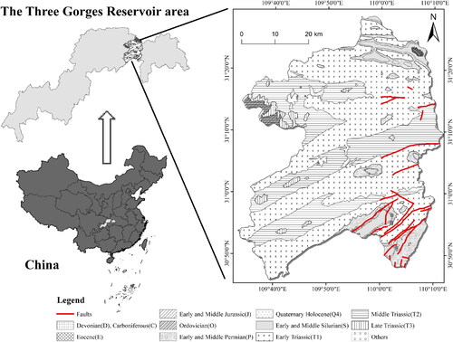
Wushan County (between 109°33′–110°11′E and 30°46′N–31°28′N) is located in the east of Chongqing, at the heart of the Three Gorges Reservoir area, known as the ‘Northeast Chongqing Portal’ (Figure 1). Its altitude ranges from 63 m to 2,688 m above the sea level, as calculated from a 30 m regular grid digital elevation model (DEM). Wushan County is located at the junction of the three structural systems of the Dabashan arc structure, the Eastern Sichuan fold belt and the Sichuan-Hubei-Hunan-Guizhou uplift fold belt, with sophisticated structural stress fields. The terrain comprises a succession of limestone ridges and gorges, with inter-gorge valleys where interbedded mudstones, shales, and thinly bedded limestones predominate (Liu et al. 2020b). Therefore, the stability of the study area is poor, coupled with rainfall softening and reservoir erosion leading to easy formation of landslides. In addition to Triassic and Permian strata, Wushan County is also distributed in Devonian, Cambrian, Eocene, etc. The geology of the area is mainly composed of a Sinian-Jurassic sedimentary, and a pre-Sinian crystalline basement. Under a humid subtropical monsoon climate and obvious three-dimensional climate characteristics, the climate of Wushan County is mild, with abundant rainfall. The annual average precipitation is 1,041 mm mild climate and mean annual temperature is 18.4 °C (Xia et al. 2018). 69% precipitation mainly occurs in summer and autumn. According to statistics (Xu et al. 2018), since 1998, there has been an increasing number of disaster zones in Wushan County, with a total of more than 6,000 houses damaged, 20,000 people affected and economic losses of more than 100 million yuan. Among them, Taping H1 landslide deformation gradually increased as a significant phenomenon (Yu et al. 2019). Therefore, how to reduce the negative impact of landslide disaster has become a major focus of local governments’ response to natural disasters.

Figure 1. Location and geological map of the study area.

Affected by complex mountainous landforms, involving lithological folds, human engineering activities, and climatic and hydrological influences, geological disasters occur frequently. The Three Gorges reservoir area has become a serious landslide disaster area (Li et al. 2019). The frequent landslides of Wushan County have greatly threatened the lives and properties of people. Since 1998, the disasters throughout the county have not diminished: more than 6,000 houses have been damaged and up to 20,000 people have been affected. There has been an economic loss of more than 100 million yuan (Liu et al. 2020a).

2.2. Landslide inventory

The preparation of a landslide inventory is a key for landslide susceptibility modeling. It can assess the relationship between landslide distribution and conditioning factors including landslides of names, geographic position, areas and other basic information. Firstly, the historical landslides come from Chongqing Municipal Geological Environment Agency. Since 2007, the geological disaster management department of Chongqing formed a geological disaster garrison (about 500 members) permanently stationed in geological disaster-prone areas. Once the landslide emergency is found, they will be responsible for the evacuation of personnel and recording basic information on the landslide. In addition, they judge the landslide type, scale, sliding direction and other basic information by landslide geological survey, engineering geophysical exploration and brick exploration. Ultimately, 1,001 landslides were identified for 2001-2016, including attribute information for landslides of names, geographic position, areas, volumes, and occurrence times. There are 963 small-medium (volume ≤100 × 10⁴ m³) and soil landslides, while there are only 38 large (volume >100 × 10⁴ m³) and rock landslides. Among the small-medium and soil landslides, there are 866 landslides whose movement typologies are slide, 92 movement typologies are flow, and 5 movement typologies are fall. Scholars have suggested that different types of landslides should be dealt with in different manners (Wang et al. 2019b), but there are only limited data on large and rock landslides and those movement typologies are flow and fall. Therefore, this research will explore small-medium, soil, and slide landslides to establish the landslide inventory, with the locations of a total of 866 of them mapped in Figure 2. Additionally, the landslide inventory showed most of the landslides that occurred on both sides of the river.

Figure 2. Distribution and on-site investigation of landslides in the study area.

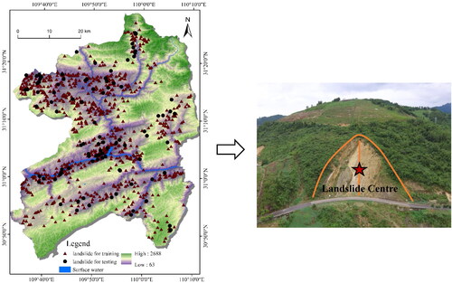
These landslides are typically small. Landslide area varies from 100 m² to 96,800 m². According to the formation mechanism of the landslide, it is found that the occurrence of a landslide is caused by the movement of a certain position rather than the entire landslide area. In the field survey, we mark the latitude and longitude of the geometric center of the landslide as the location of the landslide (Figure 2). Furthermore, this study uses two different symbols to distinguish landslide for training and testing in landslide inventory map randomly. Consequently, training datasets of landslide were used for modeling, which will make it predictive. The remaining landslides were used to test learning ability of the two models and evaluation processes. In order to obtain good fitting and prediction accuracy, distribution of the training landslide on conditioning factors and selecting a suitable method cannot be ignored (Abedini et al). Random selection is a common method, which can avoid subjectivity and enhance the learning ability of the model. All datasets were randomly classified into training (70%) and testing (30%).

2.3. Data

Except historical landslides, this paper also involves remote sensing data, topographic data, geological data, and other sources, whose types and accuracy are shown in Table 1. Baidu Map Service (http://map.baidu.com) provides POI (point of interest) data in 2016, including attractions, hospitals, universities, etc., to characterize the distribution and intensity of human infrastructure.

Table 1. Data and data sources.

Data name	Data sources	Type	Scale
Historical landslide	Chongqing Geological monitoring station	Dataset
Elevation	Aster satellite	Grid	30 m
Geological data	National Geological Data Center	Grid	1:200,000
Land cover	Chongqing Municipal Bureau of land and resources	Vector	1:100,000
Administrative division	Chongqing Municipal Bureau of land and resources	Vector	1:100,000
River network	Chongqing Water Resources Bureau	Vector	1:100,000
Annual rainfall	Chongqing Meteorological Administration	Dataset	90 m
Road	Chongqing Transportation Commission	Vector	1:100,000
Satellite image	Geospatial Data Cloud platform	Grid	30 m
POI of Chongqing	Web Crawler	Dataset

3. Methods

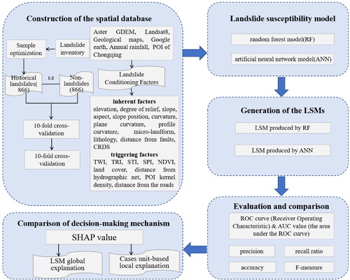
The study aims to compare the two different machine learning methods (RF and ANN) for LSM in Wushan County. The assessment procedure of this study consists of four parts: (a) construction of landslide and non-landslide spatial databases; (b) data preparation of landslide conditioning factors and construction of training test datasets in ArcGIS 10.4 software; (c) generation of the LSM; (d) evaluation and comparison of the two models (Figure 3).

Figure 3. Flowchart of the study.

3.1. Construction of the spatial database

The selection of conditioning factors directly affects the accuracy of models and LSM. Conditioning factors for landslide initiation could be classified into inherent and triggering factors. The former refers to the internal factors that play a controlling role in the occurrence of landslides, including mainly topography, geological conditions, and fault structure; the latter refers to the external factors that trigger the occurrence of landslides, such as environmental conditions and human activities (Basu and Pal 2018). Based on the principles of field investigation, satellite images, the literature review and available data, there were 22 factors selected, including the topography factors: topographic wetness index (TWI), elevation, slope position, plan curvature, aspect, slope, degree of relief, curvature, profile curvature, micro-landform, stream power index (SPI) (Basu and Pal 2018), terrain roughness index (TRI) (Althuwaynee et al. 2014), sediment transport index (STI) (Pourghasemi et al. 2012). Geological conditions factors include: distance from faults, lithology, combination reclassification of stratum dip direction and slope aspect (CRDS) (Sun et al. 2020b). Environmental conditions factors are: land cover, annual average rainfall, distance from hydrographic net, normalized vegetation index (NDVI). Human activities factors include POI kernel density and distance from roads. Particularly, point-of-interest (POI) represents the location of shops, hospitals, schools, etc., on maps; it can show information on economic society, which is closely linked to human activities (Bakillah et al. 2014). Usually, the higher the POI kernel density, the better would be the urban development in an area. It is noteworthy that previous studies have rarely considered the impact of human activities on landslides, but such activities play a non-negligible role in the occurrence of landslides (Reichenbach et al. 2018). Therefore, this research selects POI kernel density, a representative factor of the type of human activities, to represent one of the factors in human activities. The description of each factor is shown in Table 2.

Table 2. Description of landslides conditioning factors.

Influence	Conditioning factor	Description
Topography	Elevation (m)	Elevation is the basic data for extracting terrain data, usually reflecting climate and vegetation patterns (Ngo et al. 2021).
	Aspect	Aspect is defined as the direction of projection of slope normal on horizontal plane. It plays an important role in mountain ecology. The orientation of mountain has an effect on sunshine hours and solar radiation intensity (Wang et al. 2019a).
	Slope (°)	Slope refers to the degree of surface unit steepness, equal to the vertical height of the slope divided by horizontal distance (Hong et al. 2019).
	Degree of relief (m)	It is a macroscopic index that describes the topographic characteristics of a region and characterizes the potential energy of surface erosion and material movement. In a certain area, the degree of relief is equal to the maximum value of elevation minus the minimum value. Different degree of relief regions have different influence on the occurrence of landslides (Wang et al. 2020).
	Curvature	Curvature can be seen as the slope of a slope. It stresses the materials on the slope and affects the movement of water on the slope surface (Chen et al. 2021; Moosavi and Niazi 2016).
	Plan Curvature	It is the slope perpendicular to the direction of the maximum slope. A positive value indicates that the cell is part of the lateral concave slope. A negative value indicates that the slope is laterally convex (Chen et al. 2021; Moosavi and Niazi 2016).
	Profile Curvature	The change rate of elevation along the maximum direction of slope becomes profile curvature, that is, the change rate of ground slope. A positive value indicates that the cell is part of a concave up slope. A negative value indicates that the slope is raised (Chen et al. 2021; Moosavi and Niazi 2016).
	Slope position	The core work of slope position extraction is the division of landform parts and landform types (Sun et al. 2021).
	Micro-landform	Relatively small-scale geomorphologic form and the smallest geomorphologic unit (Sun et al. 2020a).
	TWI	Based on DEM data, TWI comprehensively considers the influence of topography and soil on soil moisture distribution, and has important theoretical and application value in the study of spatial distribution of soil moisture in the basin (Sun et al. 2020c).
	TRI	TRI is the surface roughness index. Based on DEM, it is an index to measure surface fluctuation and erosion degree (Pham et al. 2020).
	STI	STI is a sediment transport index, which is used to characterize the surface sediment transport and deposition (Ali et al. 2021).
	SPI	The stream power index (SPI) is used to calculate the erosion value of surface water based on DEM data. The greater the value, the more obvious the erosion of surface water flow (Zhou et al. 2021).
Geological conditions	Distance from faults(m)	Setting a buffer zone to the fault, the closer to the main fault area, the looser the slope soil, more likely to cause landslides (Yi et al. 2020).
	Lithology	There are abundant outcropped strata and many types of lithology in the study area. Due to the different degrees of weakness of various strata lithology, their shear strength is different, and the difficulty of landslide is different (Wang et al. 2021).
	CRDS	CRDS refers to the relationship between the dip angle of rock and the aspect, and the direction of the sedimentary heap (Sun et al. 2020c).
Environmental conditions	Distance from hydrographic net (m)	The study area water system to establish buffers to determine the different scope of influence. Because the bank slope is cut and eroded by water flow, the slope closer to the river is more unstable, which leads to the occurrence of landslides (Kavzoglu et al. 2015).
	NDVI	Vegetation growth is another key factor reflecting slope stability. Therefore, the normalized difference vegetation index (NDVI) was used to detect the vegetation growth status, vegetation coverage and eliminate some radiation errors (Chen et al. 2021).
	Land cover	Land cover refers to the surface complex covered by natural and artificial buildings, including vegetation, soil, lakes and various buildings, with different land stability (Wang et al. 2019a).
	Annual average rainfall (mm)	The data are derived from the average rainfall from 2000 to 2014 to reflect the long-term rainfall and distribution characteristics in the study area (Sun et al. 2022b).
Human activities	Distance from roads (m)	The construction of a large number of roads inevitably poses a threat to the stability of the slope and is easy to induce landslides (Sun et al. 2022a).
	POI kernel density	POI nuclear density covers almost all types of human engineering buildings. Similar to the construction of highways, these buildings will also loose the soil around the slope, thus affecting the slope stability (Wang et al. 2021).

DEM from ASTER GDEM was used to extract the topography factors. Land cover and NDVI come from Landsat 8 OLI satellite images. We vectorized the 1: 200,000 geological maps to obtain lithologic and faults factors. Similarly, the hydro-graphic nets and roads factors were vectorized by Google Earth images. CRDS was extracted by subtraction and reclassification of aspects and tendencies. The multi-level buffer zones are established for faults, hydrographic nets and roads to generate distances from faults, hydrographic nets and roads. Rainfall data were derived from the local climate stations and using Kriging spatial interpolation method to generate annual average rainfall factor. Lastly, Baidu Map Service provides POI records and a total of about 12,688 records in the study area, including shops, hospitals, schools, etc. POI kernel density was generated by Kernel Density tool.

In order to unify the spatial resolution of 22 landslide conditioning factors, all factors were converted to a raster grid (30 × 30 m cells) that corresponds to the DEM resolution. According to relevant literature (Huang et al. 2017), a pixel of 30 × 30 m can not only capture the spatial characteristics of a landslide in detail, but also reduce the workload and time. The acquisition path and classification of conditioning factor is directly related to their different natures. Therefore, according to references, field investigation and experts’ experience, the corresponding classification scheme for each continuous factor was established in Table 3. In short, the spatial thematic maps of landslide conditioning factors after reclassification were constructed with the grid unit of 30 m spatial resolution (Figure 4).

Figure 4. Thematic maps of landslide conditioning factors: (a) elevation; (b) slope; (c) degree of relief; (d) aspect; (e) slope position; (f) micro-landform; (g) curvature; (h) profile curvature; (i) plan curvature; (j) lithology; (k) distance from faults; (l) CRDS; (m) TRI; (n) TWI; (o) STI; (p) SPI; (q) NDVI; (r) distance from hydrographic net; (s) annual average rainfall; (t) land cover; (u) distance from roads; and (v) POI kernel density. Note: The landslide and non-landslides for testing are all displayed, while a part of landslide and non-landslides for training are selected randomly for display.

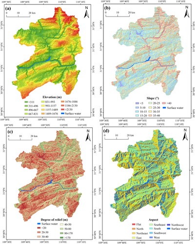
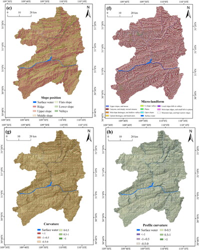
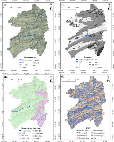
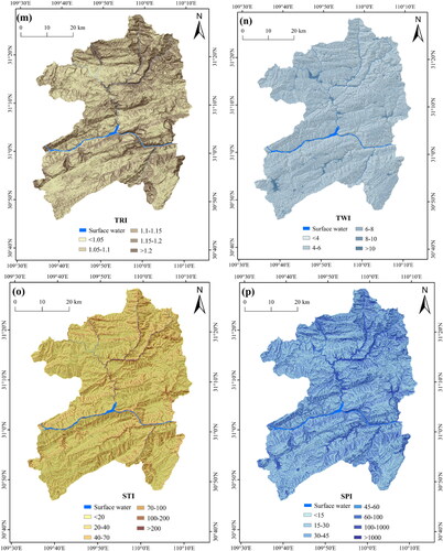
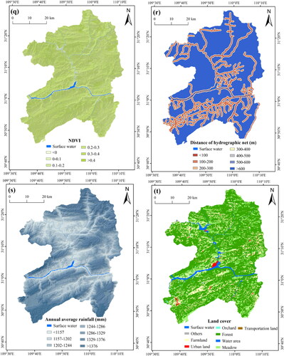
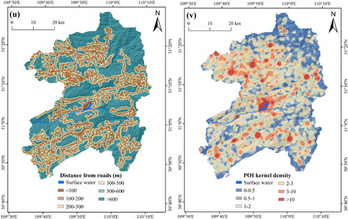
Table 3. Classification of landslide-conditioning factors.

Conditioning factor	Classification standard
Elevation (m)	1. <311; 2. 311–496; 3. 496–667; 4. 667–831; 5. 831–993; 6. 993 ∼ 1157; 7. 1157–1489; 8. 1489–1676; 9. 1676–1886; 10. 1886–2130; 11. >2130
Slope (°)	1. < 5; 2. 5–10; 3. 10–15; 4. 15–20; 5. 20–25; 6. 25–30; 7. 30–35; 8. 35–40; 9. >40
Degree of relief (m)	1. <20; 2. 20 ∼ 30; 3. 30–40; 4. 40–50; 5. 50–80; 6. 80–170; 7. >170
Aspect	1. Flat; 2. North; 3. Northeast; 4. East; 5. Southeast; 6. South; 7. Southwest; 8. West; 9. Northwest
Slope position	1. Ridge; 2. Upper slope; 3. Middle slope; 4. Flats slope; 5. Lower slope; 6. Valleys;
Micro-landform	1. Canyons, and deeply incised streams; 2. Mid-slope drainages, and shallow valleys; 3. Upland drainages, and headwaters; 4. U-shape valleys; 5. Plains; 6. Open slopes; 7. Upper slopes, and mesas; 8. Local ridges hills in valleys; 9. Mid-slope ridges, and small hills in plains; 10. Mountain tops, and high narrow ridges
Curvature	1. <-1; 2. −1–−0.5; 3. −0.5–0; 4. 0–0.5; 5. 0.5–1; 6. > 1
Profile curvature	1. <-1; 2. −1–−0.5; 3. −0.5–0; 4. 0–0.5; 5. 0.5–1; 6. > 1
Plan curvature	1. <-1; 2. −1–−0.5; 3. −0.5–0; 4. 0–0.5; 5. 0.5–1; 6. > 1
Lithology	1. D, C; 2. E; 3. J; 4. O; 5. P; 6. Q4; 7. S; 8. T1; 9. T2; 10. T3; 11. Others
Distance from faults (m)	1. < 500; 2. 50–1000; 3.1000–1500; 4. 1500–2000; 5. 2000–2500; 6. 2500–3000; 7. > 3000
CRDS	1. Dip-slope I; 2. Dip-slope II; 3. Outward slope; 4. Oblique slope; 5. Tangential slope; 6. Reverse slope; 7. Flat
TRI	1. < 1.05; 2. 1.05–1.1; 3. 1.1–1.15; 4. 1.15–1.2; 5. > 1.2
TWI	1. < 4; 2. 4–6; 3. 6–8; 4. 8–10; 5. >10
STI	1. < 20; 2. 20–40; 3. 40–70; 4. 70–100; 5. 100–200; 6. > 200
SPI	1. < 15; 2. 15–30; 3. 30–45; 4. 45–60; 5. 60–100; 6. 100–1000; 7. > 1000
NDVI	1. <0; 2. 0–0.1; 3. 0.1–0.2; 4. 0.2–0.3; 5. 0.3–0.4; 6. >0.4
Distance from hydrographic net (m)	1. < 100; 2. 100–200; 3. 200–300; 4. 300–500; 5. 500–600; 6. > 600
Annual average rainfall (mm)	1. <1157; 2. 1157–1202; 3. 1202–1244; 4. 1244–1286; 5. 1286–1329; 6. 1329–1376; 7. >1376
Land cover	1. Meadow; 2. Farmland; 3. Water area; 4. Forest; 5. Orchard; 6. Transportation land; 7. Urban land; 8. Others
Distance from roads (m)	1. <100; 2. 100–200; 3. 200–300; 4. 300–500; 5. 500–600; 6. >600
POI kernel density	1. 0–0.5; 2. 0.5–1; 3. 1–2; 4. 2–3; 5. 3–10; 6. >10

To lower the data discreteness, the classification factors were normalized (Wen 2015). Therefore, the values of each factor in different dimensions are limited to the interval [0, 1]. The normalization formula is as follows: (1) $$X^{*}=(X-X_{\min })/(X_{\max }-X_{\min })$$(1) where $X^{*}$ represents the normalized data; $X$ represents the data before normalization; $X_{\min }$ represents the minimum value of each factor; and $X_{\max }$ represents the maximum value of each factor.

3.2. Preparation of the training and testing datasets

In our study, landslide and non-landslide formed all datasets. 866 historical landslides consisted of positive cells and non-landslide served as negative cells. Additional non-landslide cells could expand the data size for machine learning, but it will cause a sample imbalance problem, thereby biasing the classifier towards the non-landslide data and negatively affecting its performance (Wang et al. 2020). After many attempts at the ratios of positive and negative cells, a balanced (1:1) positive and negative dataset has been proposed, and 866 non-landslides were randomly extracted from the non-landslide area. Then, all datasets were randomly divided into 70% (the training dataset) and 30% (the testing dataset). Specially, RF and ANN models do not need to consider the problem of multivariate collinearity in general regression analysis and the predictive ability of the two models is not affected by multicollinearity.

3.3. Landslide susceptibility models

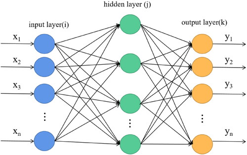
3.3.1. Artificial neural network

Artificial Neural Network (ANN) (Chakraborty and Goswami 2017; Pavel et al. 2011) is a mathematical model used for distributed parallel information processing with capability to abstracts human brain neurons from the perspective of information processing, acquire, present, and calculate mapping from data multivariate space to another. ANN is an operation model composed of a large number of interconnected nodes. Each node represents a neuron. The conversion function in the neuron is called activation function (Melchiorre et al. 2008). Without the limitations of statistical techniques of oversimplification, prohibitive data requirements and ineffective input data acquisition, ANN has a remarkable ability for handling imperfect or incomplete data and the nonlinear and complex problems.

The most prominently employed neural network method is the Back Propagation (BP) algorithm. BP neural network is a multi-layer artificial neural network, which consists of information forward propagation and error back propagation (Arora et al. 2004). The output result can be expressed by Eq. (2)(2) $$y_n=\sum _{j=1}^{N_2}{W}_{kj}f(\sum _{i=1}^{N_1}{W}_{ij}{x}_i+b_k)$$(2) : (2) $$y_n=\sum _{j=1}^{N_2}{W}_{kj}f(\sum _{i=1}^{N_1}{W}_{ij}{x}_i+b_k)$$(2) where $y_n$ is the nth output, $W_{kj}$ is weight from the k neuron in the hidden layer to the j neuron in the output layer. $f(.)$ is the transfer function of the hidden layer neuron. $b_k$ is the bias value of the k neuron in the hidden layer. $N_1$ is the number of neurons in the input layer, $N_2$ is the number of neurons in hidden layer. As long as the number of hidden layer neurons is sufficient, the BP network with a hidden layer can approximate any complex nonlinear function with arbitrary accuracy.

As shown in Figure 5, the BP neural network model comprises three layers, namely, input layer (i.e. landslide conditioning factors), hidden layers and output layer (i.e. landslide susceptibility). There are many neurons in the model which are connected in layers. ANN model is trained in R studio software.

Figure 5. BP neural network model structure.

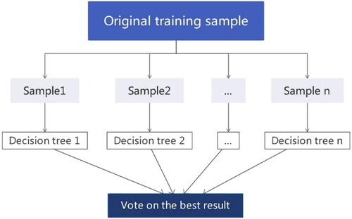
3.3.2. Random forest

Multiple decision trees are established through different data subsets, and their judgment results are voted to obtain the output results of the RF. Numerous researches indicate that the random forest has a relatively high tolerance to outliers and noises, and it is not easy to produce over-fitting (Sahin et al. 2020).

Combining N unrelated decision tree models $[h(X,{\theta }_k);k = 1,\dots \dots ]$ through classification model is the core of RF. In the model, each decision tree judges and predicts the classification of the sample (via classification algorithm). In order to improve the performance of random forest models, an irrelevant training set is established to provide differences between models. Through sample training, different classification models $h_1(X) \dots \dots h_k(X)$ are obtained, and then the random forest models are combined by using these classifications. Then to vote: (3) $$H\left(x\right)={\mathit{arg}}_z^{\max }{\Sigma }_{i=1}^{k}I\left(h_i\right(x)=Z)$$(3) where H(x) denotes a random forest model, h_i is a single decision tree model, Z denotes an output variable, and I(.) is an explicit function.

RF model is trained in R studio software. Figure 6 shows the steps of the RF algorithm.

Figure 6. The schematic diagram of the random forest (RF) algorithm.

3.4. Shapley additive explanations (SHAP)

At present, the research on landslide evaluation tends to develop models with high precision and strong generalization ability, ignoring the discussion on the internal mechanism of models. However, machine learning models lacking explanatory power are not effective in practical application. Given complex formation process of landslides, different models implement different decision-making mechanisms for the study area. Exploring the essential differences of machine learning models can contribute to improving and optimizing landslide susceptibility models. The most common interpretation methods include global interpretation and local interpretation, such as LIME and SHAP, which can be applied to any model, approaching the trained model through continuous assumptions and tests, and then speculating on the working mechanism of models. Commonly used explanatory algorithms include SHAP, LIME, and PDP, which possess better consistency with other explanatory algorithms SHAP, and can present the positive/negative relationship between each prediction factor and the target variable for local and global interpretation. For local interpretability, each feature owns a set of Shapley values that can be adopted to explain the contribution of each feature of each sample to the prediction results, thereby increasing the transparency of algorithms. Therefore, this paper discusses the decision mechanism of RF and ANN landslide susceptibility models from global and local aspects by using SHAP values, aiming to intensify the interpretability and transparency of machine learning and establish the trust relationship between landslide susceptibility models and landslide prevention and control management department.

SHAP was first proposed by Lundberg and Lee as an explanatory framework for the black box model (Lundberg and Lee 2017), with its main role to quantify the contribution of each feature to the model output. The basic idea is to calculate the marginal contribution of a feature in all feature sequences by calculating the marginal contribution of the feature when it is added to the model, namely, the Shaply value, and finally compute the mean value of all marginal contributions of the feature. $$g\left(x^{\prime }\right)={\varphi }_0+\sum _M^{j=1}\mathrm{ }{\varphi }_j$$ where $g(x^{\prime })$ is the value of the model, and ${\varphi }_0$ refers to a constant for explaining the model, that is, the predicted mean of all training samples. $\mathrm{ }{\varphi }_j$ means the attribution value of each feature (Shapley value).

3.5. Performance and validation of two models

Validation of the model is a key step to test whether the results are scientific and reasonable. Therefore, it is necessary to use different indicators and methods. In particular, the confusion matrix, receiver operating characteristic curve (ROC) and area under ROC curve (AUC) are used to evaluate the accuracy commonly, as study on landslide susceptibility is prone to be a typical binary classification problem (0,1) (Kalantar et al. 2017). Secondly, based on the confusion matrix, statistical measures such as accuracy, precision, recall, and F-measure were also used to evaluate the predictive capabilities of the models, and these measures were calculated by the following formulas: (4) $$\mathit{AUC}=\frac{(\sum TP+\sum TN)}{(P+N)}$$(4) (5) $$\mathit{Sensitivity}=\frac{TP}{TP+FN}$$(5) (6) $$\mathit{Specificity}=\frac{TN}{TN+FP}$$(6) (7) $$\mathit{Accuracy}=\frac{TP+TN}{TP+FP+TN+FN}$$(7) (8) $$\mathit{Precision}=\frac{TP}{TP+FP}$$(8) (9) $$\mathit{Recall}=\frac{TP}{TP+FN}$$(9) (10) $$\mathrm{F}-\mathrm{measure}\mathrm{ }=\frac{2\mathrm{ }\times \mathrm{ }TP}{2\times TP+FP+FN}$$(10) where $P$ is the sum of landslides, $N$ is the sum of non-landslides, $TP$ (True Positive) and $TN$ (True Negative) are the numbers of correctly classified cells, and $FP$ (False Positive) and $FN$ (False Negative) are the numbers of incorrectly classified cells. AUC between 1.0 and 0.5, in the case of AUC > 0.5, the AUC is closer to 1, indicating that the model prediction effect is better. For accuracy, precision, recall, and F-measure metrics between 0 and 1, 0 and 1 represent ideal and invalid models, respectively, and a higher value represents a better model.

4. Results and analyses

4.1. The results of LSM by different models

In order to reduce the variability and avoid over-fitting, the 10-fold cross-validation method was used to select training and testing datasets. Multiple experiments based on a large number of datasets and different techniques manifest that 10-fold cross-validation is a suitable choice for obtaining the optimal precision sample. By 10-fold cross-validation, all datasets (866 positive cells and 866 negative cells) were divided into ten individual subsets randomly and averagely. When one subset was tested, other subsets were applied for model training over 10 rounds.

The 10-fold cross-validation results of the ANN and RF model are described in Table 4. For the ANN, the accuracy of the test dataset was 0.888 averagely, and Subset 3 exhibits the highest accuracy (0.948). Therefore, Subset 3 was used to construct the ANN model. Afterwards, the established model was applied to the entire study area to obtain landslide susceptibility value. As a result, in order to facilitate the comparison of evaluation results of different models, the LSM is divided into five classes (highest 10%, second 10%, third 10%, fourth 20% and remaining 50%) by two methods of specified area ratios (Pradhan and Lee 2010), corresponding to extremely high, high, moderate, low and very low susceptibility regions, respectively. The LSM of Wushan County was generated by using the ANN model in Figure 7(a), showing that low class of landslide susceptibility in most regions of Wushan County is mainly concentrated in the east and southwest. The high susceptibility regions are mainly concentrated in Yangtze River and its tributaries, which matched well with the distribution of actual historical landslides. For the RF model, its accuracy of the test dataset was 0.996 averagely, and Subset 1dispays the highest accuracy of 1.000. Therefore, Subset 1 dataset was utilized to construct the RF model. Figure 7(b) depicts the LSM produced by the RF model for Wushan County covered with landslides, which was in good agreement with the distribution of historical landslides

Figure 7. Landslide susceptibility mappings: (a) ANN model; (b) RF model.

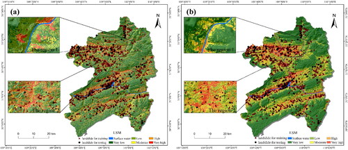
Table 4. The accuracy of 10-fold cross-validation.

Subset (ANN)	Accuracy		Subset (RF)	Accuracy
	Training dataset	Test dataset		Training dataset	Test dataset
1	0.967	0.884	1	1.000	1.000
2	0.949	0.920	2	1.000	0.995
3	0.945	0.948	3	1.000	0.994
4	0.972	0.855	4	1.000	1.000
5	0.951	0.914	5	1.000	0.990
6	0.970	0.839	6	1.000	0.995
7	0.990	0.902	7	1.000	0.990
8	0.941	0.827	8	1.000	1.000
9	0.972	0.919	9	1.000	1.000
10	0.942	0.873	10	1.000	1.000

Moreover, in order to quantitatively evaluate the effectiveness of the two models, statistical analyses were conducted on the percentage of each susceptibility classification, the number of landslides, as well as the regional proportion and density of each class (Table 5). The results of the ANN model indicated 47% of the landslides are located in 20% of high and very high susceptibility regions, but only 26% of the landslides are located in 50% of very low susceptibility regions. The evaluation outcomes revealed that the landslide density increased by approximately 5 times (from 0.145 to 0.700) as the susceptibility class varied from very low to very high, indicating that landslides are concentrated in high and extremely high susceptibility regions. According to RF model results, most areas of Wushan County are located in low susceptibility class regions; more than 73% of landslides cases are located in 20% of high and very high susceptibility regions; only 6% of landslides are located in 50% of low and very low susceptibility regions. The landslide density from 0.035 to 1.552 increased by about 44 times when the susceptibility class changed from very low to very high.

Table 5. Statistics of the susceptibility classes.

	Class:	Very low:	Low:	Moderate:	High:	Very high:
	Coverage (%)	50 %	20 %	10 %	10 %	10 %
ANN	Landslide (number)	223	124	113	173	233
	Landslide (%)	26 %	14 %	13 %	20 %	27 %
	Landslide density (Pcs/km^2)	0.145	0.234	0.461	0.605	0.700
RF	Landslide (number)	51	98	86	175	456
	Landslide (%)	6 %	11 %	10 %	20 %	53 %
	Landslide density (Pcs/km^2)	0.035	0.167	0.293	0.596	1.552

4.2. Validation and comparison

To further compare the performance of the two models, the results of confusion matrix, the ROC plots and AUC values of the two models are specified in Table 6 and Figure 8, respectively. Furthermore, precision, AUC, accuracy, recall rate and F-measure were adopted for model evaluation. The AUC of the training data and test data represents the success rate and the predictive ability of the model, respectively (Tsangaratos et al. 2017). Figure 8(a) and 8(b) show that the AUC values of ANN and RF model training data were 0.990 and 1.00, respectively, and the AUC values of test data were 0.966 and 1.00, respectively. Besides, precision, overall accuracy, recall rate, and F-measure of both ANN and RF models can be calculated simply in Table 6. For all datasets, the precision, overall accuracy, recall rate, and F-measure values of ANN model were 0.950, 0.953, 0.957, and 0.953, respectively, while the counterparts of RF model were all 1.00. All indicators demonstrate that despite reasonable goodness of fit presented by the two models, RF model embodies better performance both in training and test data sets, which further confirms RF model can achieve more ideal prediction results than ANN model.

Figure 8. ROC curve of the ANN and RF models: (a) ANN model; (b) RF model.

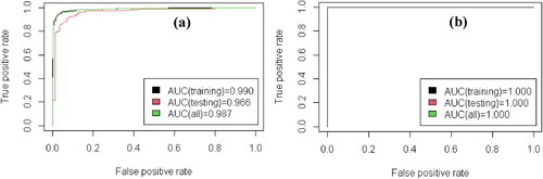
Table 6. Confusion matrix of the ANN and RF models.

Model			Actual value
			Non-landslide (0)	Landslide (1)
ANN	Predicted value	Non-landslide (0)	822	37
		Landslide (1)	44	829
RF			Non-landslide (0)	Landslide (1)
	Predicted value	Non-landslide (0)	866	0
		Landslide (1)	0	866

Also, the two models from the results of LSMs were compared. On the one hand, two regions were selected for comparison in order to display the differences between the two generated LSMs (Figure 7) more intuitively. As shown in Region 1, compared with the LSM generated by the ANN model, the accuracy of landslides falling into high and very high susceptibility regions is higher in the LSM of RF model. For Region 2, although the LSMs generated by both models almost include most of the landslides, the high-very high susceptibility regions of LSM generated by RF occupy less area. On the other hand, in LSMs, 26% of landslides are located in very low susceptibility region by ANN, while only 6% are located in the same very low susceptibility region by RF; 27% of landslides are located in very high susceptibility region by ANN, while 53% are located in the same region by RF. In general, landslides in the same area are more distributed in high and extremely high susceptibility regions in RF, while the distribution law of landslides is not obvious for the LSM generated by ANN. This certifies that the RF model outperforms the ANN model in landslide susceptibility of the whole area.

4.3. Factor importance based on SHAP value

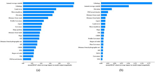
The Shapley value is used to quantify the contribution of each feature to the model prediction. As an index to judge the importance of factors, the global interpretation of the landslide susceptibility model in Wushan County is carried out, and the factor importance ranking based on ANN model and RF is obtained (Figure 9). It can be seen from Figure 9 that in the ANN model, the five factors of annual average rainfall, lithology, landcover, micro-landform and elevation exert the greatest impact on the model. As for the RF model, lithology, annual average rainfall, elevation and POI kernel density can be regarded as the most influencing factors on the model, and the average SHAP absolute value of lithology factor reaches more than 0.175, which is far higher than the importance level of other factors.

Figure 9. Factor importance ranking: (a) ANN; (b) RF.

4.4. Local explanation of the model

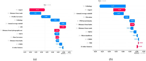
The local explanatory function of SHAP can extract the influence of each variable in the single sample observation model on the model decision, so as to reveal the decision-making mechanism of the model for this sample. A landslide case unit (Case 1) and a non-landslide case unit (Case 2) are randomly selected (Figure 10), and the waterfall plot in SHAP is used for local explanation of both RF and ANN models. The ordinate of the waterfall plot represents all variables and their values of the cases, and the abscissa represents the size of the influence of the variables on the model decision-making, with red and blue representing positive and negative impacts, separately. E[f(x)] refers to the SHAP standard value, that is, the predictive mean of this case unit. Figures 11 and 12 are the waterfall plots of two case units in RF model and ANN model respectively.

Figure 10. Selection of case units: (a) ANN; (b) RF.

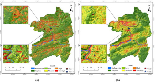
Figure 11. Waterfall plot of landslide case unit: (a) ANN; (b) RF.

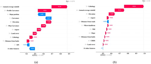
Figure 12. Waterfall plot of non-landslide case unit: (a) ANN; (b) RF.

5. Discussion

5.1. Significance of prediction framework based on ML—SHAP

In this paper, two kinds of different machine learning algorithms are employed for landslide susceptibility. The results of Figure 8 and Table 6 can confirm excellent prediction ability reflected by ANN and RF models. Meanwhile, the landslide susceptibility zoning results trained by the two models are reasonable, which are in good agreement with the distribution of historical landslide cases. However, the prediction effect of RF (AUC = 1, F-score = 1) is better than that of ANN (AUC = 0.966, F-score = 0.953). It can be seen that the AUC values of both ANN and RF models are very high. The AUC value of the RF model is 1. In machine learning, the accuracy of models not only depends on the learning algorithm, but also is affected by the selection of different parameters and factors. Sun et al. (2020a) discovered that the accuracy of models can be improved after hyperparameter optimization. It is worth noting that in spite of excellent prediction accuracy obtained by RF and ANN in Wushan County, the model fitting effect may vary due to the actual differences in topography and climatic environment in different regions. In addition, good generalization capability for LSM exhibited by machine learning has been sufficiently proved (Sun et al. 2020c). It is undeniable that both ANN and RF achieved good prediction accuracy in this study, which can be used as a reference for other areas with similar topographic conditions. In fact, both ANN and RF belong to Bagging algorithms. The Bagging method constructs multiple black-box learners on the random subset of the original training set, and then combines the prediction results of these learners to form the final prediction results. Hence, owing to the exposed disadvantage of low interpretability, ANN and RF model algorithms are usually called 'black box models’. This lack of explanatory machine learning models will pose a serious threat to the application of landslide susceptibility zoning.

Therefore, this paper proposes an interpretation framework based on SHAP value to explain the prediction mechanism of machine learning models. Firstly, the influence of each factor on the model is quantified by the average absolute value of SHAP. After that, the SHAP summary diagram can be utilized to initially excavate whether different values of each factor have a facilitating or inhibiting effect on the occurrence of landslides. Besides, SHAP can extract a single sample from the model for local explanation, which can explore the contribution of landslide impact factors to the prediction results within each evaluation unit in the study area. In the study, landslide and non-landslide samples are randomly selected for objectively studying the decision process of the model according to the waterfall plot to facilitate the scientific and comprehensive comprehension of the decision mechanism of the model during decision-making. Compared with the previous black box prediction model, the ML-SHAP interpretable landslide prediction model proposed in this paper, with its higher practicability can provide a solid basis for the occurrence of landslide disasters for disaster management departments.

Nowadays, most of the studies on machine learning in the field of landslide susceptibility have only compared the differences in prediction accuracy between different models. And there is no unanimous conclusion on which model is most suitable for landslide susceptibility zoning. Through comparison of RF and ANN algorithms, Sevgen et al. (2019) concluded that RF algorithm is more appropriate for landslide prediction. And Wang et al. (2019b) compared RF, ANN and found that the accuracy of ANN is higher. In summary, it is not sufficient to compare only the prediction accuracy of models. The explanatory ability of models should be considered in the pursuit of high prediction performance models, and the reasonableness of model prediction results can be verified with the help of local explanatory results of models. The article proposes an interpretable model based on SHAP and machine learning to reveal the decision mechanism of different machine learning prediction models through the global and local interpretation of the model.

5.2. Influence factors on model

Figure 13 shows the summary plot of SHAP values for feature importance ranking of two prediction models, which combines the influence of feature weight and feature value on the model. Each unit on the graph indicates a Shapley value of a certain feature of an instance. The position on the y-axis is determined by the feature, and the position on the x-axis is determined by the Shapley value. The color represents the eigenvalues from small to large, and the overlapping points float in the y-axis direction. Therefore, the distribution of Shapley values for each feature can be clearly captured. From the summary plot, it can be concluded that factors such as annual average rainfall, elevation and POI kernel density have roughly the same influence on both ANN and RF models. Specifically, annual average rainfall and elevation are negatively correlated with the predicted value of the model, and POI kernel density is positively correlated with the predicted probability of the model. The reason for this phenomenon is that annual average rainfall data are measured based on long-term observation, including unstable rocks and soil carried away by surface runoff from rainfall. Annual average rainfall not only eroded the slope, but also affected the development of vegetation on the slope, thus affecting the occurrence of landslides. As a typical mountainous area with complex terrain, low-elevation areas in Wushan County are often characterized with looser soil bed and more human engineering activities. Therefore, the most intensive elevation range of landslide distribution was the low-elevation range with frequent human activities and low vegetation coverage. Due to low vegetation coverage and weak water and soil fixation ability in areas with high POI density, strong human engineering activities will inevitably destroy the slope stability, leading to greater possibility of landslides.

Figure 13. Summary plot of SHAP values: (a) ANN; (b) RF.

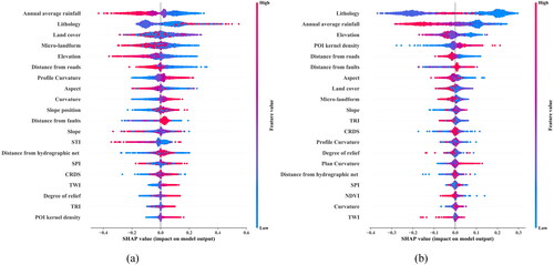
In addition, as can be seen from the summary plot of SHAP values, the difference between the two models in the aspect of lithology factor is that in the context of high lithology value, the ANN model tends to judge it as a factor that promotes landslide occurrence, and in some sample cases, this factor plays a great role in the decision-making of the ANN model. The SHAP value reaches more than 0.4, and the SHAP value of the lithology factor with the same value in the RF model is less than 0.3. The RF model is sensitive to the lithology factor in the middle position, and the SHAP value in some samples reaches-0.35, while the SHAP value in the ANN model is only between −0.2 and 0.

5.3. Decision differences of different models for the same sample

As can be seen from Figure 11, for Case 1, the predicted values of RF model and ANN model are 0.99 and 0.878, respectively. Meanwhile, both models judge Case 1 as landslide, which is consistent with the actual situation of Case 1. Although both models correctly predict the occurrence of landslide, the selected model decision-making mechanisms are inconsistent. The same characteristics of the same unit have different contributions in the two models. The lithology of sample 1 is E, which plays the most important role in the RF model, with the model contribution value of 0.24. As for the ANN model, the contribution of lithology to the prediction results is small, with the contribution value of only 0.04. Besides, the average annual rainfall value of sample 1 was 1244-1286 mm, which occupied a significant position in both models. The contribution values in RF model and ANN model were 0.11 and 0.18, respectively.

For randomly selected non-landslide sample cases (Sample 2), the prediction probabilities of RF and ANN models are 0.23 and 0.33, respectively. Despite correct prediction of the slope by both models, the influence factors play different roles in the decision-making process of the model. In RF, the most influential factors on the model decision-making results include lithology, aspect and annual average rainfall. In ANN, factors exerting the greatest impact on the model involve slope aspect, distance from roads and profile curvature. In the RF model, lithology has a great influence on the model, with the contribution value to the results calculated as −0.19, while in the ANN model, the contribution value of lithology to the model is −0.08. Distance from the road has a small contribution to the decision-making results of the model in RF, with the contribution value of only −0.02. However, this factor has a large contribution to the decision-making results of the model in ANN, with the contribution value of 0.1. For the same sample, different models can result in different influence directions on the prediction results. The distance between sample 2 and fault is greater than 3000 m. In the RF model, the distance between sample 2 and fault is 3000 m, with the contribution value to the results computed as 0.03, which promotes the occurrence of landslide. Whereas, in the ANN model, the distance of 3000 m between sample 2 and the fault brings an inhibitory effect on the occurrence of landslide through measuring the contribution value to the results as −0.03.

According to local interpretation results of the two samples, the RF model is highly sensitive to lithology. Whether landslide samples or non-landslide samples, lithology factor always plays the most important role in the model, and the contribution value of this factor to the model is far higher than other factors. In addition, it can be concluded that different models adopt different decision-making mechanisms for the same sample, which is manifested in different contribution values of the unified characteristics of different models in the model decision-making process, resulting in the differences in the final prediction results of different models. The main reason for this phenomenon is different decision-making mechanisms operated within the model. RF is deemed as a set of decision trees, each of which is highly independent, able to predict landslide susceptibility without restriction. ANN is a network model composed of connected neurons that are grouped by layers to process the data of each layer, and then pass it on to the next layer. The prediction results are only determined by the last layer of neurons.

6. Conclusion

This paper aims to figure out the most suitable landslide susceptibility model and explore the difference of internal decision mechanism of different models. A new interpretable landslide susceptibility model is developed for ANN and RF models using SHAP values, which is applied to 866 historical landslide events in Wushan County. The primary conclusions are as follows:

(1) Through comparison of the two models, the AUC values of the test data of ANN and RF models were calculated as 0.966 and 1.00, respectively. As for the LSM generated by the ANN model, 47% landslides are located in 20% of high and very high susceptibility regions, but only 26% landslides are located in 50% of very low susceptibility regions. On the other hand, for the LSM produced by the RF model, more than 73% of landslides are located in 20% of high and very high susceptibility regions, but 6% landslides in 50% of low and very low susceptibility regions. In a word, both models in this study present excellent performances, but there is no denying that the RF model exhibits better stability and robustness.

(2) For the same study area, different models have different decision mechanisms. Specifically, the contribution of the same influencing factor in different models is disparate, and different models provide different decision-making bases for the same case unit. RF model is extremely sensitive to lithological factors.

(3) The interpretable landslide susceptibility model proposed in this paper is capable of model explanation at both global and local levels. The model can not only explore the importance of factors, but also promote the in-depth study on the contribution of different values of the same feature to the model, thereby laying a good decision-making foundation for each evaluation unit. The interpretable landslide susceptibility prediction framework can provide a reasonable reference for government departments to prevent and control landslide disasters.

Data availability statement

The data presented in this study can be available on request from the corresponding author.

Disclosure statement

The authors declare no conflict of interest.

Additional information

Funding

The research reported in this manuscript is funded by the Natural Science Foundation of Chongqing (Grants No. CSTB2022NSCQ-MSX0594) and Humanities and Social Sciences Research Project of the Ministry of Education (Grants No. 16YJCZH061).

References

- Akinci H, Zeybek M. 2021. Comparing classical statistic and machine learning models in landslide susceptibility mapping in Ardanuc (Artvin), Turkey. Nat Hazards. 108(2):1515–1543.
- Ali SA, Parvin F, Vojtekova J, Costache R, Linh NTT, Pham QB, Vojtek M, Gigovic L, Ahmad A, Ghorbani MA. 2021. GIS-based landslide susceptibility modeling: a comparison between fuzzy multi-criteria and machine learning algorithms. Geosci Front. 12(2):857–876.
- Althuwaynee OF, Pradhan B, Park H-J, Lee JH. 2014. A novel ensemble bivariate statistical evidential belief function with knowledge-based analytical hierarchy process and multivariate statistical logistic regression for landslide susceptibility mapping. Catena. 114:21–36.
- Arora MK, Das Gupta AS, Gupta RP. 2004. An artificial neural network approach for landslide hazard zonation in the Bhagirathi (Ganga) Valley, Himalayas. Int J Remote Sens. 25(3):559–572.
- Aslam B, Zafar A, Khalil U. 2022. Comparison of multiple conventional and unconventional machine learning models for landslide susceptibility mapping of Northern part of Pakistan. Environ Dev Sustain. 1–28.
- Bakillah M, Liang S, Mobasheri A, Arsanjani JJ, Zipf A. 2014. Fine-resolution population mapping using OpenStreetMap points-of-interest. Int J Geogr Inf Sci. 28(9):1940–1963.
- Basu T, Pal S. 2018. Identification of landslide susceptibility zones in Gish River basin, West Bengal, India. Georisk: Assess Manage Risk Eng Syst Geohazards. 12(1):14–28.
- Chakraborty A, Goswami D. 2017. Prediction of slope stability using multiple linear regression (MLR) and artificial neural network (ANN). Arab J Geosci. 10(17):385.
- Chen W, Chen X, Peng JB, Panahi M, Lee S. 2021. Landslide susceptibility modeling based on ANFIS with teaching-learning-based optimization and Satin bowerbird optimizer. Geosci Front. 12(1):93–107.
- de Oliveira GG, Ruiz LFC, Guasselli LA, Haetinger C. 2019. Random forest and artificial neural networks in landslide susceptibility modeling: a case study of the Fao River Basin, Southern Brazil. Nat Hazards. 99(2):1049–1073.
- Harmouzi H, Nefeslioglu HA, Rouai M, Sezer EA, Dekayir A, Gokceoglu C. 2019. Landslide susceptibility mapping of the Mediterranean coastal zone of Morocco between Oued Laou and El Jebha using artificial neural networks (ANN). Arab J Geosci. 12(22):696.
- Hong HY, Shahabi H, Shirzadi A, Chen W, Chapi K, Bin Ahmad B, Roodposhti MS, Hesar AY, Tian YY, Bui DT. 2019. Landslide susceptibility assessment at the Wuning area, China: a comparison between multi-criteria decision making, bivariate statistical and machine learning methods. Nat Hazards. 96(1):173–212.
- Huang F, Yin K, Huang J, Gui L, Wang P. 2017. Landslide susceptibility mapping based on self-organizing-map network and extreme learning machine. Eng Geol. 223:11–22.
- Huang FM, Cao ZS, Guo JF, Jiang SH, Li S, Guo ZZ. 2020a. Comparisons of heuristic, general statistical and machine learning models for landslide susceptibility prediction and mapping. Catena. 191:104580.
- Huang FM, Cao ZS, Jiang SH, Zhou CB, Huang JS, Guo ZZ. 2020b. Landslide susceptibility prediction based on a semi-supervised multiple-layer perceptron model. Landslides. 17(12):2919–2930.
- Huang FM, Pan LH, Fan XM, Jiang SH, Huang JS, Zhou CB. 2022. The uncertainty of landslide susceptibility prediction modeling: suitability of linear conditioning factors. Bull Eng Geol Environ. 81(5):182.
- Huang FM, Ye Z, Jiang SH, Huang JS, Chang ZL, Chen JW. 2021. Uncertainty study of landslide susceptibility prediction considering the different attribute interval numbers of environmental factors and different data-based models. Catena. 202:105250.
- Huang R, Li W. 2011. Formation, distribution and risk control of landslides in China. J Rock Mech Geotech Eng. 3(2):97–116.
- Kalantar B, Pradhan B, Naghibi SA, Motevalli A, Mansor S. 2017. Assessment of the effects of training data selection on the landslide susceptibility mapping: a comparison between support vector machine (SVM), logistic regression (LR) and artificial neural networks (ANN). Geomat Nat Haz Risk. 9(1):49–69.
- Kavzoglu T, Sahin EK, Colkesen I. 2015. Selecting optimal conditioning factors in shallow translational landslide susceptibility mapping using genetic algorithm. Eng Geol. 192:101–112.
- Li C, Fu Z, Wang Y, Tang H, Yan J, Gong W, Yao W, Criss RE. 2019. Susceptibility of reservoir-induced landslides and strategies for increasing the slope stability in the Three Gorges Reservoir Area: Zigui Basin as an example. Eng Geol. 261:105279.
- Liu R, Shi S, Sun D, Xu J. 2020a. Based on GIS and random forest model for landslide susceptibility mapping in Wushan county. J Chongqing Nor Univ (Nat Sci). 37:86–96.
- Liu X, Jing R, Miao L, Han Y, Ddeng Z, Xiong C. 2020b. Reconstruction models and typical case analysis of the fluctuation belt of reservoir bank slopes in Wushan. Chin J Rock Mech Eng. 39:1321–1332.
- Lombardo L, Mai PM. 2018. Presenting logistic regression-based landslide susceptibility results. Eng Geol. 244:14–24.
- Lundberg SM, Lee S-I. 2017. A unified approach to interpreting model predictions. Adv Neural Inf Process Syst. 30:1–10.
- Melchiorre C, Matteucci M, Azzoni A, Zanchi A. 2008. Artificial neural networks and cluster analysis in landslide susceptibility zonation. Geomorphology. 94(3–4):379–400.
- Mondal S, Mandal S. 2018. RS & GIS-based landslide susceptibility mapping of the Balason River basin, Darjeeling Himalaya, using logistic regression (LR) model. Georisk: Assess Manage Risk Eng Syst Geohazards. 12(1):29–44.
- Moosavi V, Niazi Y. 2016. Development of hybrid wavelet packet-statistical models (WP-SM) for landslide susceptibility mapping. Landslides. 13(1):97–114.
- Ngo PTT, Panahi M, Khosravi K, Ghorbanzadeh O, Kariminejad N, Cerda A, Lee S. 2021. Evaluation of deep learning algorithms for national scale landslide susceptibility mapping of Iran. Geosci Front. 12(2):505–519.
- Pavel M, Nelson JD, Jonathan Fannin R. 2011. An analysis of landslide susceptibility zonation using a subjective geomorphic mapping and existing landslides. Comput Geosci. 37(4):554–566.
- Petley D. 2012. Global patterns of loss of life from landslides. Geology. 40(10):927–930.
- Pham BT, Trung NT, Qi CC, Phong TV, Dou J, Ho LS, Le HV, Prakash I. 2020. Coupling RBF neural network with ensemble learning techniques for landslide susceptibility mapping. Catena. 195:104805.
- Pourghasemi HR, Mohammady M, Pradhan B. 2012. Landslide susceptibility mapping using index of entropy and conditional probability models in GIS: Safarood Basin, Iran. Catena. 97:71–84.
- Pradhan B, Lee S. 2010. Landslide susceptibility assessment and factor effect analysis: backpropagation artificial neural networks and their comparison with frequency ratio and bivariate logistic regression modelling. Environ Model Softw. 25(6):747–759.
- Reichenbach P, Rossi M, Malamud BD, Mihir M, Guzzetti F. 2018. A review of statistically-based landslide susceptibility models. Earth-Sci Rev. 180:60–91.
- Sahin EK, Colkesen I, Kavzoglu T. 2018. A comparative assessment of canonical correlation forest, random forest, rotation forest and logistic regression methods for landslide susceptibility mapping. Geocarto Int. 35(4):341–363.
- Sevgen E, Kocaman S, Nefeslioglu HA, Gokceoglu C. 2019. A novel performance assessment approach using photogrammetric techniques for landslide susceptibility mapping with logistic regression, ANN and random forest. Sensors. 19(18):3940.
- Sun D, Gu Q, Wen H, Xu J, Zhang Y, Shi S, Xue M, Zhou X. 2022a. Assessment of landslide susceptibility along mountain highways based on different machine learning algorithms and mapping units by hybrid factors screening and sample optimization.
- Sun D, Wen H, Wang D, Xu J. 2020a. A random forest model of landslide susceptibility mapping based on hyperparameter optimization using Bayes algorithm. Geomorphology. 362:107201.
- Sun D, Wen H, Zhang Y, Xue M. 2020b. An optimal sample selection-based logistic regression model of slope physical resistance against rainfall-induced landslide. Nat Hazards. 105(2):1255–1279.
- Sun DL, Gu QY, Wen HJ, Shi SX, Mi CL, Zhang FT. 2022b. A hybrid landslide warning model coupling susceptibility zoning and precipitation. Forests. 13(6):827.
- Sun DL, Xu JH, Wen HJ, Wang DZ. 2021. Assessment of landslide susceptibility mapping based on Bayesian hyperparameter optimization: a comparison between logistic regression and random forest. Eng Geol. 281:105972.
- Sun DL, Xu JH, Wen HJ, Wang Y. 2020c. An optimized random forest model and its generalization ability in landslide susceptibility mapping: application in two areas of Three Gorges Reservoir, China. J Earth Sci. 31(6):1068–1086.
- Tsangaratos P, Ilia I, Hong H, Chen W, Xu C. 2016. Applying Information Theory and GIS-based quantitative methods to produce landslide susceptibility maps in Nancheng County, China. Landslides. 14(3):1091–1111.
- Wang Y, Fang ZC, Hong HY. 2019a. Comparison of convolutional neural networks for landslide susceptibility mapping in Yanshan County, China. Sci Total Environ. 666:975–993.
- Wang Y, Sun DL, Wen HJ, Zhang H, Zhang FT. 2020. Comparison of random forest model and frequency ratio model for landslide susceptibility mapping (LSM) in Yunyang County (Chongqing, China). IJERPH. 17(12):4206.
- Wang Y, Wen H, Sun D, Li Y. 2021. Quantitative assessment of landslide risk based on susceptibility mapping using random forest and GeoDetector. Remote Sens. 13(13):2625.
- Wang Y, Wu X, Chen Z, Ren F, Feng L, Du Q. 2019b. Optimizing the predictive ability of machine learning methods for landslide susceptibility mapping using SMOTE for Lishui City in Zhejiang Province, China. IJERPH. 16(3):368.
- Wen H. 2015. A susceptibility mapping model of earthquake-triggered slope geohazards based on geo-spatial data in mountainous regions. Georisk: Assess Manage Risk Eng Syst Geohazards. 9(1):25–36.
- Xia H, Yin K, Liang X, Ma F. 2018. Landslide susceptibility assessment based on SVM-ANN Models: a case study for Wushan County in the Three Gorges Reservoir. Chin J Geol Haz Control. 29:13–19.
- Xu CC, Sun Q, Yang XY. 2018. A study of the factors influencing the occurrence of landslides in the Wushan area. Environ Earth Sci. 77(11):406.
- Yi YN, Zhang ZJ, Zhang WC, Jia HH, Zhang JQ. 2020. Landslide susceptibility mapping using multiscale sampling strategy and convolutional neural network: a case study in Jiuzhaigou region. Catena. 195:104851.
- Yu LB, Cao Y, Zhou C, Wang Y, Huo ZT. 2019. Landslide susceptibility mapping combining information gain ratio and support vector machines: a case study from Wushan Segment in the Three Gorges Reservoir Area, China. Applied Sciences-Basel. 9(22):4756.
- Zhao QF, Chen W, Peng CH, Wang DZ, Xue WF, Bian HY. 2022. Modeling landslide susceptibility using an evidential belief function-based multiclass alternating decision tree and logistic model tree. Environ Earth Sci. 81(15):404.
- Zhou X, Wen H, Zhang Y, Xu J, Zhang W. 2021. Landslide susceptibility mapping using hybrid random forest with GeoDetector and RFE for factor optimization. Geosci Front. 12(5):101211.
- Zhou X, Wen H, Li Z, Zhang H, Zhang W. 2022. An interpretable model for the susceptibility of rainfall-induced shallow landslides based on SHAP and XGBoost. Geocarto Int. DOI: 10.1080/10106049.2022.2076928.