Urban surface water bodies mapping using the automatic k-means based approach and sentinel-2 imagery

Abstract

Rivers, lakes, and open water bodies play crucial roles in environmental development, especially in urban ecosystems. Accurate urban surface water body maps in high resolution are an important prerequisite for better and faster decision making for urban ecosystem monitoring, mitigating the effects of urban heat islands and urban climate change adaptation. Research presents new automatic algorithm for urban surface bodies mapping (AUWM). Algorithm was tested on Sentinel-2 data and can be applied globally for automatic mapping water bodies in 10-m spatial resolution. AUWM was developed based on modified normalized difference water index, pansharpening techniques (MNDWI_PS), and k-means clustering algorithm. Research was provided on three study sites. The optimal number of classes for k-means in AUWM is four. Accuracy assessment results show that AUWM is a highly accurate method for water bodies mapping, confirmed by all statistical parameters; accuracy, kappa, precision, and F1 value are 0.997, 0.830, 0.998, and 0.998, respectively.

Keywords:

• Unsupervised classification
• k-means
• Sentinel-2
• urban water bodies
• automatic mapping

1. Introduction

Water is a multi-faceted natural resource (Singh et al. 2009). Overexploitation, changes in land-use/land-cover, and climate change adversely impact the hydrological cycle, ultimately affecting the availability of surface and groundwater on Earth. Water plays a crucial role for urban ecosystems and urban climate (Xiang et al. 2021; Krauze and Wagner 2019; Nakayama and Hashimoto 2011; Arnfield 2003), especially in purpose of mitigating the effects of urban heat islands (Nwakaire et al. 2020; Ghosh and Das 2018; Steeneveld et al. 2014; Nakayama and Fujita 2010; Ichinose et al. 1999) and urban climate change adaptation (Golfam et al. 2021; Larson et al. 2015; Gober and Kirkwood 2010). Knowledge of the distribution of rivers and lakes at different spatial and temporal scales is critical for understanding the water, energy, and nutrient cycles at local, regional, and global scales (Rosinger et al. 2020; Yamazaki et al. 2015; Allen and Pavelsky 2015; Downing et al. 2012). Reliable estimates of surface water are critically important for different scientific disciplines. Using open access and operational satellite data, we can map, extract and monitor open water resources to cater to human needs and to achieve sustainability. Changes in the areas or volumes of water bodies can be detected by comparing satellite images of an area from different time periods or by using different classifiers (Sagan et al. 2020; Zhou et al. 2017). Optical remote sensing has many spectral channels that help to improve the accuracy of automatic mapping of urban surface water and decrease its limitations for mapping surface water when weather conditions are poor. Many methods proposed in the literature, such as single band density slicing (Kutser et al. 2020; Zhou et al. 2017; Xu 2006), unsupervised and supervised classification (Bangira et al. 2019; Zhou et al. 2017), spectral water indices, and threshold-based approaches (Li et al. 2016a; Ji et al. 2015; Xie et al. 2014; Li et al. 2013a; Hui et al. 2008; Xu 2006), are available for extracting water bodies from remote sensing images. For mapping water bodies today, many authors used various supervised machine learning methods, e.g. random forest (Wangchuk and Bolch 2020), Support vector machines (Liu et al. 2020) XGBoost (Chatufale et al. 2022). On the other hand, unsupervised classification methods do not require any training samples and are more suitable for developing automatized algorithms. K-means method is one of the most used unsupervised classification methods in remote sensing and introduced by Hartigan and Wong 1979. Still today, many authors use it for providing unsupervised classification (Gašparović et al. 2019; Tang et al. 2019; Leichtle et al. 2017; Yu et al. 2017; Zhong et al. 2017; Li et al. 2016b) or developing fully automatic methods for mapping the environment (Guo et al. 2021; Kusak et al. 2021; Ren et al. 2020; Sinaga and Yang 2020; Li et al. 2018). Gašparović et al. 2019 proposed a novel algorithm for automatic cost-effective method for land cover classification (ALCC). ALCC was developed based on an interesting, unique idea of using various spectral indices for mapping various land cover types based on unsupervised k-means classification. Real classes were determined by the median value of spectral index, e.g. class with higher vegetation indices median value represents vegetation, while the class with higher water indices median value represents water bodies. Many researchers have proposed spectral indices, such as the normalized difference water index (NDWI, McFeeters 1996), the modified normalized difference water index (MNDWI, Hu 20006), and the automated water extraction index (AWEI, Feyisa et al. 2014) to identify surface water bodies. Gudelj et al. 2018 test the accuracy analysis of inland waters detection using various water indices (AWEI, NDWI, MNDWI). The results show that MNDWI overperformed in the accuracy of all other water spectral indices for the detection inland waters.

Xie et al. (2016) used the Landsat 8 OLI sensor and developed an automatic subpixel water mapping method (ASWM) for urban areas. They first extracted mixed land-water pixels and pure water pixels and spectral linear mixture analysis was applied on the mixed land-water pixels to separate the water abundant pixels. Verpoorter et al. (2012) developed an approach, called the GeoCoverTM Water bodies Extraction Method (GWEM), that combines remote sensing and GIS to extract water bodies using Landsat 7 Enhanced Thematic Mapper Plus (ETM +) data. They describe the six steps of the GWEM approach as follows: (1) thresholding and classification; (2) texture analysis (filtering, segmentation); (3) vectorization, and (4) shadow removal. Yang et al. (2017) conducted a study to evaluate the performance of the Sentinel-2 Multispectral Instrument (MSI) imagery for mapping urban surface water using an image sharpening approach and principal component analysis. Yang and Chen (2017) proposed an automatic framework that integrates pixel-level threshold adjustment and object-oriented segmentation to map urban surface water. Their findings suggest that the object-level modified normalized difference water index (MNDWI with band 11) and the automated water extraction index are feasible for urban surface water mapping using Sentinel-2 MSI imagery. Yamazaki et al. (2015) developed an automated algorithm to process multi-temporal Landsat images and produced a Global, 3 arc-second Water Body Map (G3WBM), which delineates river channels and flood plains. Pekel et al. (2016) provide high-resolution water surface change maps from 1984 to 2015 (v1.0) based on Landsat imageries. Their new 30-m water body maps (v1.1) known as Global Surface Water Dataset (GSWD) were globally available for the period from 1984 to 2018 on the website (http://global-surface-water.appspot.com) and Google Earth Engine platform (GEE). Although many above mentioned authors have dealt with mapping water bodies, proposed algorithms are almost always based on supervised classification methods that require ground truth data and expert knowledge and effort. Therefore, a lack of research devoted to developing fully automated algorithms was observed, which, as expected, represents a scientific gap that can be solved with this research.

Main goal of this research is to develop unsupervised and totally automatic algorithm for urban surface bodies mapping for Sentinel-2 data. Specific objectives of this research are as follows: (1) to investigate the use of the spectral index method for automatic urban surface water bodies mapping; (2) to test four different variants of input bands used in k-means classification; (3) to find an optimal number of k-means classes for automatic urban surface bodies mapping and (4) to quantitatively evaluate the accuracy of our proposed urban surface water bodies mapping using optical-based water detection algorithm for Sentinel-2 data.

2. Materials and methods

2.1. Study areas and data

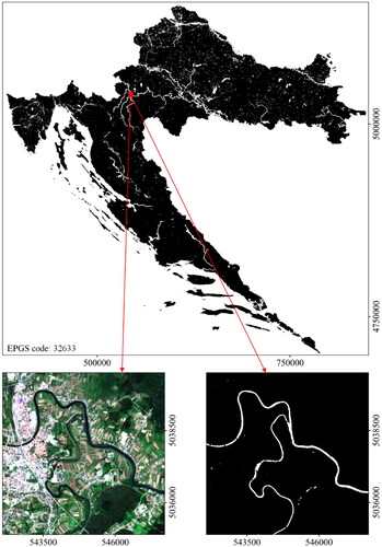
To test the robustness and applicability of the algorithm developed, three independent urban study areas were selected for mapping of urban surface water body. One study area was in Croatia and two were in India (Figure 1). Each study area represents different landscapes with different geographical and climatic characteristics and are familiar to the authors. Considering the importance of water bodies on the quality of life in big cities, proposed algorithm was tested on two capitals (New Delhi and Zagreb). Both capitals cities are lies on rivers, Yamuna in New Delhi, and Sava River in Zagreb). Zagreb also has a large number of artificial lakes such as Bundek and Jarun. Bhopal, Madhya Pradesh is known as the ‘City of Lakes’ and have various natural and artificial lakes, and one of the greenest cities in India and therefore it is chosen for the third study site. All study areas have the same dimensions of 50 km x 50 km.

Figure 1. (a) Geographic location of the study areas; (b) satellite image of the Zagreb, Croatia study area (SA1); (c) satellite image of the New Delhi, India study area (SA2); (d) satellite image of the Bhopal, Madhya Pradesh, India study area (SA3). All satellite images use the Sentinel-2 ‘true color’ composite (4–3–2).

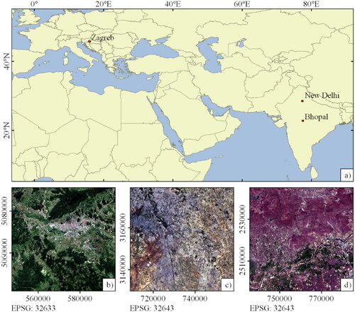
In this research, three cloud-free Sentinel-2 imagery was used (Table 1). Sentinel-2 images were downloaded via the Copernicus Open Access Hub (https://scihub.copernicus.eu/dhus/). All Sentinel-2 images were obtained using the Sentinel-2 satellite and downloaded as a Level-2A product that provides Bottom of Atmosphere reflectance values.

Table 1. Description of Sentinel-2 satellite imagery used in this research.

Study area	Sensing date	Satellite imagery ID
Zagreb, Croatia	27-July-2019	S2A_MSIL2A_20190627T095031_N0212_R079_T33TWL_20190627T142308
New Delhi, India	09-July-2019	S2A_MSIL2A_20190609T052651_N0212_R105_T43RGM_20190609T091600
Bhopal, India	27-May-2019	S2A_MSIL2A_20190527T051651_N0212_R062_T43QGF_20190527T093017

Independent, high-resolution data, e.g. Google Earth maps; commercial, very high-resolution satellite imagery, e.g. PlanetScope and WorldView and field data were collected and used for creating ground-truth raster map. Ground-truth raster map was obtained by manually verified and corrected land-cover classification. Ground-truth raster map was used for accuracy assessment of developed algorithm.

2.2. Algorithm for automatic urban surface water bodies mapping (AUWM)

2.2.1. Spectral index

To emphasize one land-cover class over others, many authors have commonly used certain spectral indices (Gašparović et al. 2019; Li et al. 2017a; Jiang et al. 2008; Zhao and Chen 2005 Gao 1996; Tucker 1979). Currently, a large number of spectral indices are used; i.e. to emphasize vegetation, Tucker (1979) suggest using the normalized difference vegetation index (NDVI). For bare land, Zhao and Chen (2005) emphasize using the normalized difference bareness index (NDBaI) and Li et al. (2017a) emphasize using the normalized difference bare land index (NBLI). For water extraction, Gao (1996) proposed the normalized difference water index (NDWI) and Xu (2006) suggest using the modified normalized difference water index (MNDWI), respectively. In this research, the MNDWI was used to extract water bodies, following previous research that tested the MNDWI (Acharya et al. 2018; Feyisa et al. 2014; Wang et al. 2013; Xu 2006) and other research that suggested using the MNDWI to map water bodies (Gašparović et al. 2019; Gudelj et al. 2018). Li et al. (2013b) defined the MNDWI as follows: (1) $$\text{MNDWI}=\frac{\text{Green}-\text{SWIR}1}{\text{Green}+\text{SWIR}1},$$(1) where SWIR1 and Green represents Sentinel-2 bands 11 (central wavelength = 1610 nm, ESA 2015) and 3 (central wavelength = 560 nm, ESA 2015), respectively.

2.2.2. Pansharpening

Considering Sentinel-2 bands 3 and 11 have different spatial resolutions (band 3 has a 10 m resolution and band 11 has a 20 m resolution, ESA 2015), MNDWI can be calculated in two ways, as follows:

1. The MNDWI can be calculated without pansharpening (MNDWI), based on the 10 m band 3 and the source band 11, which has a 20 m spatial resolution.

2. The MNDWI can be calculated with pansharpening (MNDWI_PS), based on the 10 m band 3 and the fused (i.e. pansharpened) 10 m band 11. Following the methods of Gašparović and Jogun (2018), pansharpened band 11 was calculated based on the 10 m Sentinel-2 band 8 (the spectral band closest to band 11). Therefore, the MNDWI can be calculated at a 10 m spatial resolution (MNDWI_PS).

2.2.3. K-Means clustering

Although the k-means method was introduced in remote sensing (Jain 2010, Wang 1990, Hartigan and Wong 1979) a long time ago, many authors use it today as a basis for the development unsupervised classification (Gašparović et al. 2019; Tang et al. 2019; Leichtle et al. 2017; Yu et al. 2017; Zhong et al. 2017; Li et al. 2016b) or fully automatic methods for mapping the state of the environment (Guo et al. 2021; Kusak et al. 2021; Ren et al. 2020; Sinaga and Yang 2020; Li et al. 2018). Main goal of this research is to develop unsupervised, and totally automatic algorithm for urban surface bodies mapping for Sentinel-2 data. According to previous research (Gašparović et al. 2019), a novel algorithm for automatic urban surface water bodies mapping was based on the k-means unsupervised classification. Fuelled by scientific curiosity, this research tested four different variants of input bands used in k-means classification.

1. K-means calculated by a single MNDWI band (without pansharpening, see 2.2.2.).

2. K-means calculated by a single MNDWI_PS band (with pansharpening, see 2.2.2.).

3. K-means calculated by the MNDWI band and an additional four 10 m Sentinel-2 bands (2, 3, 4 and 8, which represent the blue, green, red and near infra-red – NIR bands, respectively).

4. K-means calculated by the MNDWI_PS band and an additional four 10 m Sentinel-2 bands (2, 3, 4, and 8).

The essential input to k-means classification along with the bands is the a priori number of classes (clusters) into which the k-means method will automatically classify the entire satellite image. For that reason, the analysis used to determine the optimal class number for k-means classification was provided. For each of the above-mentioned four variations, the k-means classification was calculated based on various number of a priori classes (2, 3, 4, …, 9, 10). A total of 36 rasters were calculated based on the AUWM for each study area. Optimal number of k-means classes was chosen by combination of the highest accuracy with the least necessary processing time.

After performing the k-means classification, the proposed algorithm for automatic urban surface water bodies mapping automatically extracted the water bodies from the entire satellite imagery as the k-means class that had the highest mean value for bands MNDWI or MNDWI_PS. Additional to k-means calculated by the single MNDWI band, and accordingly to our previous research (Gašparović et al. 2019), we decide to use source Sentinel-2 bands to potentially improve final algorithm accuracy. All available 10 m Sentinel-2 bands (2, 3, 4 and 8) were selected and used for this purpose.

Main result and goal of this research is to develop unsupervised and totally automatic algorithm for urban surface bodies mapping (AUWM) for Sentinel-2 data in 10-m resolution globally. Application the AUWM algorithm for mapping water surface mapping at national scale will be presented for entire Croatia. Algorithm was realized in R programming language, version 3.4.1. (R Core Team 2017), through RStudio version 1.0.143.

2.3. Accuracy assessment

The accuracy assessment was based on a wall-to-wall comparison of the AUWM results and the land-cover classification obtained by manually verified and corrected land-cover classification made based Support Vector Machine (SVM) supervised classification method and the same satellite imagery. This approach was used to provide accuracy assessment over the entire 50 km x 50 km study areas. All pixels in the study area were used for accuracy assessment. For each study site, 25 million pixels were tested based on the ground-truth raster map. Ground-truth raster map was obtained by manually verified and corrected land-cover classification. Independent, high-resolution data, e.g. Google Earth maps; commercial, very high-resolution satellite imagery, e.g. PlanetScope and WorldView and field data were used to collect the training and test samples for land-cover classification. For land-cover classification training, 70% of all reference samples were used and for the test, 30% were used. The land-cover classification was made by 10-m Sentinel-2 bands (2, 3, 4, and 8) and a Support Vector Machine (SVM) supervised classification algorithm. Before further use, the accuracy of the land-cover classification was checked with the test samples. For all three study areas, the overall accuracy of the land-cover classification was higher than 90% with kappa higher than 0.85. The SVM classification method was chosen according to many studies, in which SVM achieved a higher accuracy for land-cover mapping than other classification methods (Thanh Noi and Kappas 2017; Qian et al. 2014). Therefore, consistent with previous research (Gašparović et al. 2019; Singh et al. 2018; Baskan et al. 2017; Rawat and Kumar 2015; Singh et al. 2014), the satellite imagery was classified into five land-cover classes: 1 – water; 2 – built-up; 3 – barren land; 4 – low vegetation; and 5 – high vegetation. The ground-truth water class used in the accuracy assessment was extracted from the land-cover classification. Finally, 10-m ground-truth water/other raster was manually verified and corrected based on the independent, very high-resolution satellite imagery (PlanetScope and WorldView).

Further, comparative assessment of developed AUWM was done by comparison with high-resolution water maps downloaded from the Global Surface Water Dataset (GSWD) website (http://global-surface-water.appspot.com, Pekel et al. 2016). GSWD water body maps were downloaded for the last available year (2018), in 30-m spatial resolution. For accuracy assessment, GSWD data were upsampled to the 10-m because AUWM and ground-truth raster were in 10-m spatial resolution. The statistical parameters for the accuracy assessment of the GSWD and AUWM were calculated based on the confusion matrix obtained by tested raster and the ground-truth water/other raster. A total of 75 million pixels from all study areas were used for comparative assessment. The main goal of this comparative assessment of the AUWM and GSWD is not the direct accuracy comparison than the representation of the importance of developing and using the AUWM that allows accurate detection of water surfaces in 10-m resolution globally. In this research, various accuracy assessment parameters were used: the accuracy (i.e. overall accuracy (Congalton and Green 2002), kappa (Congalton and Green 2002), specificity (Akobeng 2007), precision (Goutte and Gaussier 2005), F1 (i.e. F-score, Goutte and Gaussier 2005), prevalence (Kuhn 2019), McNemar’s test P value (Agresti and Kateri 2011), detection rate (Kuhn 2019), and balanced accuracy (Kuhn 2019). The algorithms for automatic urban surface water bodies mapping, as well as for accuracy assessment, were created using the R programming language, version 3.4.1. (R Core Team 2017), through RStudio version 1.0.143.

3. Results

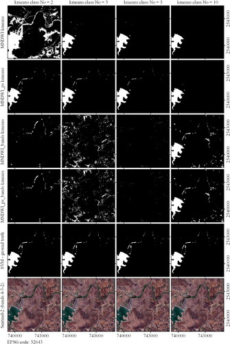
All four variants of the input bands, described in Section 2.2.3., were used to map water bodies based on the AUWM automatically. The statistical parameters for the accuracy assessments of the four variations in the AUWM, calculated based on various numbers of k-means classes (2—10), for SA1, SA2, and SA3 are shown in Figures 2, 3, and 4, respectively. The visual analyses of the AUWM results calculated by the 2, 3, 5 and 10 k-means classes for SA1, SA2, and SA3 are shown in Appendix on Figures A1, A2, and A3, respectively.

Figure 2. Statistical parameters for the accuracy assessments of the four variations in the AUWM calculated based on various numbers of k-means classes for SA1.

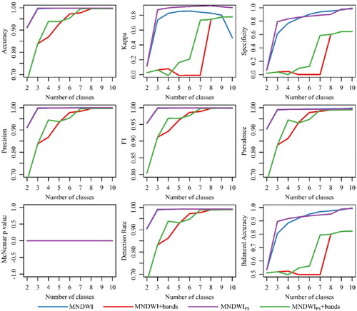
Figure 3. Statistical parameters for the accuracy assessment of the four variations in the AUWM calculated based on the various numbers of k-means classes for SA2.

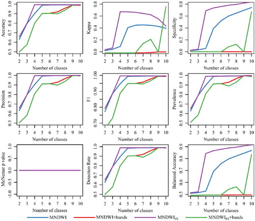
Figure 4. Statistical parameters for the accuracy assessment of the four variations in the AUWM calculated based on the various numbers of k-means classes for SA3.

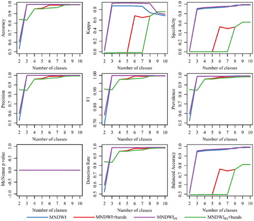
Figure 5 shows that a higher number of k-means classes in the AUWM increases the processing time. As expected, the usage of additional bands (MNDWI + band, MNDWI_PS+bands) in the AUWM increases time used (Figure 5). The accuracy assessment analyses presented in Figures 2, 3, and 4 show that the MNDWI + band, as well as the MNDWI_PS+bands have lower accuracies and lower values of the other statistical parameters relative to those of the MNDWI and MNDWI_PS. Furthermore, visual analyses in Figures A1, A2, and A3 in Appendix show many gross errors in the detection of water bodies in the MNDWI + band and MNDWI_PS+bands. Almost all statistical parameters in Figures 2, 3, and 4 show that the MNDWI_PS has a slightly higher accuracy than the MNDWI. The optimal number of classes for k-means for the MNDWI_PS should be four (Table 2, grey shaded column).

Figure 5. Processing time of the four variations in the AUWM, calculated based on the various numbers of k-means classes for (a) SA1, (b) SA2, (c) SA3, and (d) the average processing time of all three study areas.

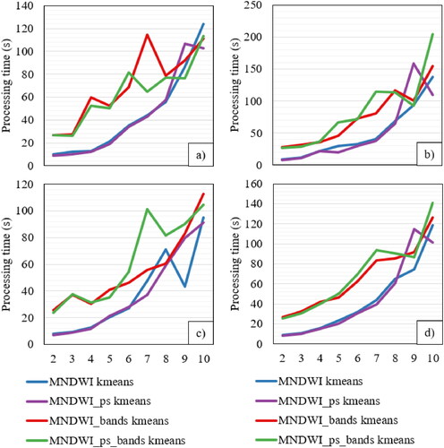
Table 2. Comparison of the statistical parameters and processing times for the MNDWI_PS calculated based on the various numbers of k-means classes. Bolded values represent lowest processing time MNDWI_PS with highest statistical parameters. Gray shaded column represents optimal number of classes for k-means for the MNDWI_PS.

k-means classes no.	2	3	4	5	6	7	8	9	10
Time(s)	8.05	9.94	15.07	20.14	30.58	39.36	60.42	114.81	101.23
Accuracy	0.73	0.93	1.00	1.00	1.00	1.00	1.00	1.00	1.00
Kappa	0.06	0.62	0.83	0.83	0.83	0.83	0.82	0.73	0.68
Specificity	0.04	0.58	0.82	0.84	0.86	0.88	0.89	0.93	0.94
Precision	0.72	0.93	1.00	1.00	1.00	1.00	1.00	1.00	1.00
F1	0.83	0.96	1.00	1.00	1.00	1.00	1.00	1.00	1.00
Prevalence	0.72	0.92	0.99	0.99	0.99	0.99	0.99	0.99	1.00
McNemar p value	0.00	0.00	0.00	0.00	0.00	0.00	0.00	0.00	0.00
Detection Rate	0.72	0.92	0.99	0.99	0.99	0.99	0.99	0.99	0.99
Balanced Accuracy	0.52	0.79	0.91	0.92	0.93	0.94	0.94	0.96	0.97

Comparative assessment shows that the AUWM has higher accuracy than the GSWD based on all statistical parameters (Figure 6).

Figure 6. Statistical parameters for the accuracy assessment of the GSWD and AUWM calculated for all study areas.

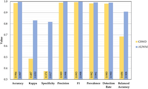
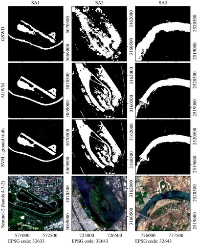
One of the main reasons for AUWM's higher accuracy compared to the GSWD is that GSWD is obtained by Landsat 30-m spatial resolution satellite imagery, while the AUWM is obtained by Sentinel-2 10-m satellite imagery. Furthermore, the visual comparison of the GSWD and AUWM for all study areas is shown in Figure 7.

Figure 7. Visual comparison of the GSWD and AUWM for all study areas.

The global application of the AUWM was done for entire territory of Republic of Croatia (Figure 8).

Figure 8. Surface water map for Croatia made using the AUWM. The enlarged subset (right) shows the area of Karlovac, known as the city situated on four rivers. Sentinel-2 ‘true color’ composite (4–3–2) was used for the comparison.

4. Discussion

The use of satellite images to generate global and regional land-cover data sets has gained interest in the scientific community in the last few decades. The accurate extraction of urban surface water will help to achieve the global United Nations sustainable development goals. Accurate and automatic generated urban surface water maps in high resolution can help researchers and policy makers for better and faster decision making in the purpose of urban ecosystem monitoring, mitigating the effects of urban heat islands (Nakayama and Fujita 2010; Steeneveld et al. 2014) and urban climate change adaptation (Larson et al. 2015; Gober and Kirkwood 2010). Satellite data can classified by considering the different steps described here, namely the election of training samples, image preprocessing, feature extraction, selection of suitable classification approaches, post-classification processing, and accuracy assessment (Gašparović et al. 2019; Lu and Weng 2007).

The spectral index has the capability to extract the feature, but they also have a similar value of different land cover classes or overlapping with other land cover classes (Szabó et al. 2016). The spectral index is commonly used to separate water and non-water classes based on spectral dissimilarity. The spectral indices (MNDWI), principal component, random forest, and support the vector machine-based method showed a more accurate separation of water versus non-water or saturated soil classes (Balázs et al. 2018). The NDWI and the MNDWI outline water from non-water areas. The MNDWI acts as an important tool for environmental monitoring and efficiently helps to delineate water areas. The spectral indices (NDVI and MNDWI) used to extract the vegetation and surface water characteristics of an aquatic system and develop the level of sedimentation risk index model (Szabó et al. 2020). The normalized analysis of the MNDWI image and the final surface water map demonstrates the effectiveness of the proposed MNDWI-based and pansharpening-based approaches (MNDWI_PS).

In this research, we have selected three geographically distinct areas and have applied an automatic urban surface water bodies mapping algorithm to extract the inland waters. The surface water map created by the AUWM has a 10 m x 10 m spatial resolution. Previous relevant studies have suggested that the MNDWI is more suitable for extracting water and has good accuracy compared to the NDWI (Du et al. 2016; Singh et al. 2015; Du et al. 2014; Li et al. 2013a; Xu 2006). The most commonly used satellite data for water resource mapping is Landsat series data; however, Landsat images have a 30 m spatial resolution and are unable to be used to identify smaller-sized open water bodies and small pools in urban areas, whereas SPOT6/7, IKONOS and Quick-bird are able to be used to map small water bodies due to their fine resolution. Modifications of the NDWI to fine spatial resolutions are limited due to the non-availability of the SWIR band (Du et al. 2016).

A comparison of the accuracy was performed on the spectral index, the MNDWI without pansharpening, the MNDWI with pansharpening and the k-means based on single MNDWI band, the k-means based on single MNDWI_PS band, the k-means calculated by MNDWI band and the additional four 10 m Sentinel-2 bands (2, 3, 4 and 8, which represent the blue, green, red and near infra-red – NIR bands, respectively) and the k-means calculated by the MNDWI_PS band and the additional four 10 m Sentinel-2 bands (2, 3, 4, and 8). This research was conducted using the Sentinel-2 10 m spectral resolution satellite imagery. High spatial resolution satellite images (RapidEye, PlanetScope, WorldView, etc.) classified by the object-based approach offer a promising solution for increasing the classification accuracy (Myint et al. 2011). The object-based approach may be able to improve this algorithm (AUWM) in the future; in the current form, it is a pixel-based AUWM. A key advantage of the algorithm is the use of fusion (pansharpening) methods to improve the spatial resolution of the SWIR1 band that is needed to calculate the MNDWI to avoid disturbances from urbanized lands (Xu 2006). The problem of mixed water and vegetation pixels can be reduced by involving the enhanced vegetation index and the normalized difference vegetation index (Menarguez 2015). The algorithm developed has some minor problems (which are very rare) with very dark shadows in cities. We have not tested our methodology for the seasonality and persistence in the water surface extraction and mapping. In future research, we could use other free or commercial satellite imagery (e.g. PlanetScope, RapidEye, etc.) that do not have SWIR1 bands to pansharpen the Sentinel-2 SWIR1 band to a higher resolution. Independent comparative assessment provided in this research shows that developed AUWM has higher accuracy than the GSWD published in the scientific journal Nature (Pekel et al. 2016). This research work indicates the importance of this research and the large applicability potential of AUWM for mapping water bodies in 10-m spatial resolution globally. The developed method will help in developing the pragmatic policies to understand in a better way in the presence of available water resources in a river basin or lake during drought and extreme conditions. This knowledge is crucial for the purpose of developing a sustainable environment in urban areas, as well as urban climate change adaptation (Li et al. 2017b; Larson et al. 2015; Wouters et al. 2015; Steeneveld et al. 2014).

AUWM was developed as a pixel-based approach and to further improve the accuracy, a similar algorithm can be developed based on the object-based approach in the future. Also, AUWM enables rapid and accurate global mapping of urban water surfaces; therefore, it can be easily applied in future research related to monitoring water bodies over a longer time series.

5. Conclusions

Open access satellite data help in mapping and monitoring of surface water. In the research presented here, we have used Sentinel-2 satellite data for three geographically distinct locations to map surface water bodies with improved accuracy. The modified normalized difference water index, pansharpening techniques (MNDWI_PS), and a k-means clustering algorithm were used to extract an enhanced urban surface water map. Proposed, a totally automatic algorithm for urban surface bodies mapping (AUWM) can be used for high accurate water bodies mapping, which is confirmed by all statistical parameters; accuracy, kappa, precision, F1 value are 0.997, 0.830, 0.998, 0.998, respectively. For developing AUWM, various number of k-means classes were used (2—10). The best variant for input band combination for AUWM was pansharpened MNDWI raster (MNDWI_PS), and the optimal number of classes for k-means is four. The algorithm has very limited uncertainty in classifying very small urban surfaces as water bodies. Independent comparative assessment provided in this research shows that developed AUWM has slightly higher accuracy than the GSWD. The global application of the AUWM was done for entire territory of Republic of Croatia. Accurate automatic created urban surface water maps generated by means of the AUWM method are an important prerequisite for better and faster decision making in the purpose of urban ecosystem monitoring, mitigating the effects of urban heat islands and urban climate change adaptation.

Disclosure statement

No potential conflict of interest was reported by the authors.

Additional information

Funding

The authors would like to thank the University of Zagreb that funded the RS4ENVIRO project entitled: ‘Advanced photogrammetry and remote sensing methods for environmental change monitoring’ (Grant No. RS4ENVIRO) and European Space Agency that funded the RS4ENVIRO project entitled: ‘Automatic monitoring of narrow-leaved ash (Fraxinus angustifolia Vahl) forests by remote sensing methods and Copernicus data’ (Grant No. RS4EST) under which this research was conducted. The authors would like to thank the European Space Agency for providing the Sentinel data free of charge.

Appendix

Figure A1. Visual analyses of the four variations in the AUWM, calculated based on the various numbers of k-means classes (2, 3, 5, and 10) for SA1.

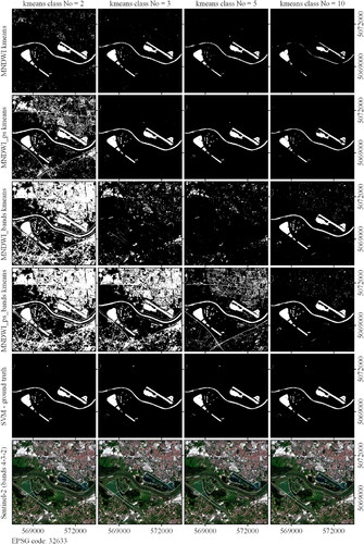
Figure A2. Visual analyses of the four variations in the AUWM, calculated based on the various numbers of k-means classes (2, 3, 5, and 10) for SA2.

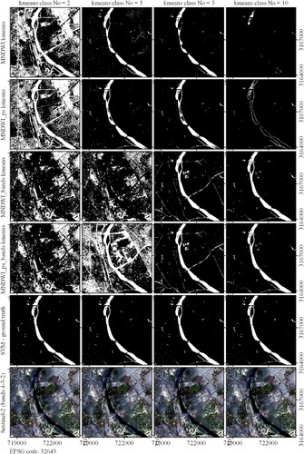
Figure A3. Visual analyses of the four variations in the AUWM, calculated based on the various numbers of k-means classes (2, 3, 5, and 10) for SA3.

References

- Acharya T, Subedi A, Lee D. 2018. Evaluation of water indices for surface water extraction in a Landsat 8 scene of Nepal. Sensors. 18(8):2580.
- Agresti A, Kateri M. 2011. Categorical data analysis BT. In: lovric, M., editor. International Encyclopedia of Statistical Science. Berlin Heidelberg: Springer; p. 206–208.
- Akobeng AK. 2007. Understanding diagnostic tests 1: sensitivity, specificity and predictive values. Acta Paediatr. 96(3):338–341.
- Allen GH, Pavelsky TM. 2015. Patterns of river width and surface area revealed by the satellite-derived North American River Width data set. Geophys Res Lett. 42(2):395–402.
- Arnfield AJ. 2003. Two decades of urban climate research: a review of turbulence, exchanges of energy and water, and the urban heat island. Int J Climatol. 23(1):1–26.
- Bangira T, Alfieri SM, Menenti M, Van Niekerk A. 2019. Comparing thresholding with machine learning classifiers for mapping complex water. Remote Sens. 11(11):1351.
- Balázs B, Bíró T, Dyke G, Singh SK, Szabó S. 2018. Extracting water-related features using reflectance data and principal component analysis of Landsat images. Hydrol Sci J. 63(2):269–284.
- Baskan O, Dengiz O, Demirag İT. 2017. The land productivity dynamics trend as a tool for land degradation assessment in a dryland ecosystem. Environ Monit Assess. 189(5):1–21.
- Chatufale AP, Rege PP, Bhatt A. 2022. Extraction of waterbody using object-based image analysis and XGBoost. Advanced Machine Intelligence and Signal Processing. Singapore: Springer; p. 341–350.
- Congalton R, Green K. 2002. Assessing the accuracy of remotely sensed data: principles and practices.
- Downing JA, Cole JJ, Duarte CM, Middelburg JJ, Melack JM, Prairie YT, Kortelainen P, Striegl RG, McDowell WH, Tranvik LJ. 2012. Global abundance and size distribution of streams and rivers. IW. 2(4):229–236.
- Du Y, Zhang Y, Ling F, Wang Q, Li W, Li X. 2016. Water bodies’ mapping from sentinel-2 imagery with modified normalized difference water index at 10-m spatial resolution produced by sharpening the SWIR band. Remote Sens. 8(4):354.
- Du Z, Li W, Zhou D, Tian L, Ling F, Wang H, Gui Y, Sun B. 2014. Analysis of Landsat-8 OLI imagery for land surface water mapping. Remote Sens Lett. 5(7):672–681.
- ESA. 2015. Sentinel-2 user handbook. Paris, France: European Space Agency (ESA).
- Feyisa GL, Meilby H, Fensholt R, Proud SR. 2014. Automated water extraction index: a new technique for surface water mapping using Landsat imagery. Remote Sens. Environ. 140:23–35.
- Gao BC. 1996. NDWI – a normalized difference water index for remote sensing of vegetation liquid water from space. Remote Sens Environ. 58(3):257–266.
- Gašparović M, Jogun T. 2018. The effect of fusing Sentinel-2 bands on land-cover classification. Int J Remote Sens. 39(3):822–841.
- Gašparović M, Zrinjski M, Gudelj M. 2019. Automatic cost-effective method for land cover classification (ALCC). Comput Environ Urban Syst. 76:1–10.
- Gober P, Kirkwood CW. 2010. Vulnerability assessment of climate-induced water shortage in Phoenix. Proc Natl Acad Sci USA. 107(50):21295–21299.
- Goutte C, Gaussier E. 2005. A probabilistic interpretation of precision, recall and F-score, with implication for evaluation. Lect Notes Comput Sci. 3408:345–359.
- Golfam P, Ashofteh PS, Loáiciga HA. 2021. Modeling adaptation policies to increase the synergies of the water-climate-agriculture nexus under climate change. Environ Dev. 37:100612.
- Ghosh S, Das A. 2018. Modelling urban cooling island impact of green space and water bodies on surface urban heat island in a continuously developing urban area. Model Earth Syst Environ. 4(2):501–515.
- Gudelj M, Gašparović M, Zrinjsk M. 2018. Accuracy analysis of the inland waters detection. International Multidisciplinary Scientific GeoConference Surveying Geology and Mining Ecology Management, SGEM. International Multidisciplinary Scientific Geoconference; p. 203–210.
- Guo Z, Shi Y, Huang F, Fan X, Huang J. 2021. Landslide susceptibility zonation method based on C5. 0 decision tree and K-means cluster algorithms to improve the efficiency of risk management. Geosci Front. 12(6):101249.
- Hartigan JA, Wong MA. 1979. Algorithm AS 136: a k-means clustering algorithm. J Royal Statist Soc. Series c (Applied Statistics). 28(1):100–108.
- Hui F, Xu B, Huang H, Yu Q, Gong P. 2008. Modelling spatial‐temporal change of Poyang Lake using multitemporal Landsat imagery. Int. J. Remote Sens. 29(20):5767–5784.
- Ichinose T, Shimodozono K, Hanaki K. 1999. Impact of anthropogenic heat on urban climate in Tokyo. Atmos Environ Pergamon. 33(24–25):3897–3909.
- Jain AK. 2010. Data clustering: 50 years beyond K-means. Pattern Recognit Lett. 31(8):651–666.
- Ji L, Geng X, Sun K, Zhao Y, Gong P. 2015. Target detection method for water mapping using Landsat 8 OLI/TIRS imagery. Water. 7(12):794–817.
- Jiang Z, Huete AR, Didan K, Miura T. 2008. Development of a two-band enhanced vegetation index without a blue band. Remote Sens Environ. 112(10):3833–3845.
- Krauze K, Wagner I. 2019. From classical water-ecosystem theories to nature-based solutions—contextualizing nature-based solutions for sustainable city. Sci Total Environ. 655:697–706.
- Kuhn M. 2019. Package ‘caret’. Classification and regression training, R Foundation for statistical computing. The R Journal. 223(7):1–224. http://free-cd.stat.unipd.it/web/packages/caret/caret.pdf
- Kusak L, Unel FB, Alptekin A, Celik MO, Yakar M. 2021. Apriori association rule and K-means clustering algorithms for interpretation of pre-event landslide areas and landslide inventory mapping. Open Geosci. 13(1):1226–1244.
- Kutser T, Hedley J, Giardino C, Roelfsema C, Brando VE. 2020. Remote sensing of shallow waters – a 50 year retrospective and future directions. Remote Sens Environ. 240:111619.
- Larson K, White D, Gober P, Wutich A. 2015. Decision-making under uncertainty for water sustainability and urban climate change adaptation. Sustainability. 7(11):14761–14784.
- Leichtle T, Geiß C, Wurm M, Lakes T, Taubenböck H. 2017. Unsupervised change detection in VHR remote sensing imagery – an object-based clustering approach in a dynamic urban environment. Int J Appl Earth Obs Geoinf. 54:15–27.
- Li Y, Martinis S, Plank S, Ludwig R. 2018. An automatic change detection approach for rapid flood mapping in Sentinel-1 SAR data. Int J Appl Earth Obs Geoinf. 73:123–135.
- Li H, Wang C, Zhong C, Su A, Xiong C, Wang J, Liu J. 2017a. Mapping urban bare land automatically from Landsat imagery with a simple index. Remote Sens. 9(3):249.
- Li F, Liu X, Zhang X, Zhao D, Liu H, Zhou C, Wang R. 2017b. Urban ecological infrastructure: an integrated network for ecosystem services and sustainable urban systems. J Clean Prod. 163: S12–S18.
- Li W, Qin Y, Sun Y, Huang H, Ling F, Tian L, Ding Y. 2016a. Estimating the relationship between dam water level and surface water area for the Danjiangkou Reservoir using Landsat remote sensing images. Remote Sens Lett. 7(2):121–130.
- Li Y, Tao C, Tan Y, Shang K, Tian J. 2016b. Unsupervised multilayer feature learning for satellite image scene classification. IEEE Geosci Remote Sens Lett. 13(2):157–161.
- Li W, Du Z, Ling F, Zhou D, Wang H, Gui Y, Sun B, Zhang X. 2013a. A comparison of land surface water mapping using the normalized difference water index from TM, ETM + and ALI. Remote Sens. 5(11):5530–5549.
- Li P, Jiang L, Feng Z. 2013b. Cross-comparison of vegetation indices derived from Landsat-7 enhanced thematic mapper plus (ETM+) and Landsat-8 operational land imager (OLI) sensors. Remote Sens. 6(1):310–329.
- Liu Q, Huang C, Shi Z, Zhang S. 2020. Probabilistic river water mapping from Landsat-8 using the support vector machine method. Remote Sens. 12(9):1374.
- Lu D, Weng Q. 2007. A survey of image classification methods and techniques for improving classification performance. Int J Remote Sens. 28(5):823–870.
- McFeeters SK. 1996. The use of the Normalized Difference Water Index (NDWI) in the delineation of open water features. Int J Remote Sens. 17(7):1425–1432.
- Menarguez MA. 2015. Global water body mapping from 1984 to 2015 using global high resolution multispectral satellite imagery. Norman, USA: University of Oklahoma.
- Myint SW, Gober P, Brazel A, Grossman-Clarke S, Weng Q. 2011. Per-pixel vs. object-based classification of urban land cover extraction using high spatial resolution imagery. Remote Sens. Environ. 115(5):1145–1161.
- Nakayama T, Fujita T. 2010. Cooling effect of water-holding pavements made of new materials on water and heat budgets in urban areas. Landsc Urban Plan. 96(2):57–67.
- Nakayama T, Hashimoto S. 2011. Analysis of the ability of water resources to reduce the urban heat island in the Tokyo megalopolis. Environ Pollut. 159(8–9):2164–2173.
- Nwakaire CM, Onn CC, Yap SP, Yuen CW, Onodagu PD. 2020. Urban heat island studies with emphasis on urban pavements: a review. Sustain Cities Soc. 63:102476.
- Qian Y, Zhou W, Yan J, Li W, Han L. 2014. Comparing machine learning classifiers for object-based land cover classification using very high resolution imagery. Remote Sens. 7(1):153–168.
- Pekel JF, Cottam A, Gorelick N, Belward AS. 2016. High-resolution mapping of global surface water and its long-term changes. Nature. 540(7633):418–422.
- Rawat JS, Kumar M. 2015. Monitoring land use/cover change using remote sensing and GIS techniques: a case study of Hawalbagh block, district Almora, Uttarakhand, India. Egypt J Remote Sens Sp Sci. 18(1):77–84.
- Rosinger AY, Brewis A, Wutich A, Jepson W, Staddon C, Stoler J, Young SL. 2020. Water borrowing is consistently practiced globally and is associated with water-related system failures across diverse environments. Glob Environ Change. 64:102148.
- R Core Team. 2017. R: a language and environment for statistical computing. Vienna, Austria: R Foundation for Statistical Computing.. https://cran.microsoft.com/snapshot/2014-09-08/web/packages/dplR/vignettes/xdate-dplR.pdf
- Ren Z, Sun L, Zhai Q. 2020. Improved k-means and spectral matching for hyperspectral mineral mapping. Int J Appl Earth Obs Geoinf. 91:102154.
- Sagan V, Peterson KT, Maimaitijiang M, Sidike P, Sloan J, Greeling BA, Maalouf S, Adams C., 2020. Monitoring inland water quality using remote sensing: potential and limitations of spectral indices, bio-optical simulations, machine learning, and cloud computing. Earth Sci Rev. 205:103187.
- Sinaga KP, Yang MS. 2020. Unsupervised K-means clustering algorithm. IEEE Access. 8:80716–80727.
- Singh SK, Laari PB, Mustak S, Srivastava PK, Szabó S. 2018. Modelling of land use land cover change using earth observation data-sets of Tons River Basin, Madhya Pradesh, India. Geocarto Int. 33(11):1202–1222.
- Singh KV, Setia R, Sahoo S, Prasad A, Pateriya B. 2015. Evaluation of NDWI and MNDWI for assessment of waterlogging by integrating digital elevation model and groundwater level. Geocarto Int. 30(6):650–661.
- Singh SK, Srivastava PK, Gupta M, Thakur JK, Mukherjee S. 2014. Appraisal of land use/land cover of mangrove forest ecosystem using support vector machine. Environ Earth Sci. 71(5):2245–2255.
- Singh S, Singh C, Kumar K, Gupta R, Mukherjee S. 2009. Spatial-temporal monitoring of groundwater using multivariate statistical techniques in Bareilly district of Uttar Pradesh. India J Hydrol Hydromech. 57:45–54.
- Szabó L, Deák B, Bíró T, Dyke GJ, Szabó S. 2020. NDVI as a proxy for estimating sedimentation and vegetation spread in artificial lakes—monitoring of spatial and temporal changes by using satellite images overarching three decades. Remote Sens. 12(9):1468.
- Szabó S, Gácsi Z, Balázs B. 2016. Specific features of NDVI, NDWI and MNDWI as reflected in land cover categories. Acta Geogr Landsc Environ. 10(3–4):194–202.
- Steeneveld GJ, Koopmans S, Heusinkveld BG, Theeuwes NE. 2014. Refreshing the role of open water surfaces on mitigating the maximum urban heat island effect. Landsc Urban Plan. 121:92–96.
- Tang T, Chen S, Zhao M, Huang W, Luo J. 2019. Very large-scale data classification based on K-means clustering and multi-kernel SVM. Soft Comput. 23(11):3793–3801.
- Thanh Noi P, Kappas M. 2017. Comparison of random forest, k-nearest neighbor, and support vector machine classifiers for land cover classification using Sentinel-2 imagery. Sensors. 18(2):18.
- Tucker CJ. 1979. Red and photographic infrared linear combinations for monitoring vegetation. Remote Sens Environ. 8(2):127–150.
- Verpoorter C, Kutser T, Tranvik L. 2012. Automated mapping of water bodies using Landsat multispectral data. Limnol Oceanogr Methods. 10(12):1037–1050.
- Wangchuk S, Bolch T. 2020. Mapping of glacial lakes using Sentinel-1 and Sentinel-2 data and a random forest classifier: strengths and challenges. Sci Remote Sens. 2:100008.
- Wang F. 1990. Improving remote sensing image analysis through fuzzy information representation. Photogramm Eng Remote Sens. 56(8):1163–1169.
- Wang Y, Huang F, Wei Y. 2013. Water body extraction from LANDSAT ETM + image using MNDWI and K-T transformation. International Conference on Geoinformatics.
- Wouters H, Demuzere M, Ridder KD, Van Lipzig NPM. 2015. The impact of impervious water-storage parametrization on urban climate modelling. Urban Clim. 11:24–50.
- Xiang X, Li Q, Khan S, Khalaf OI. 2021. Urban water resource management for sustainable environment planning using artificial intelligence techniques. Environ Impact Assess Rev. 86:106515.
- Xie H, Luo X, Xu X, Pan H, Tong X. 2016. Automated subpixel surface water mapping from heterogeneous urban environments using Landsat 8 OLI imagery. Remote Sens. 8(7):584.
- Xie H, Luo X, Xu X, Tong X, Jin Y, Pan H, Zhou B. 2014. New hyperspectral difference water index for the extraction of urban water bodies by the use of airborne hyperspectral images. J Appl Remote Sens. 8(1):85098.
- Xu H. 2006. Modification of normalised difference water index (NDWI) to enhance open water features in remotely sensed imagery. Int J Remote Sens. 27(14):3025–3033.
- Yamazaki D, Trigg MA, Ikeshima D. 2015. Development of a global ∼90m water body map using multi-temporal Landsat images. Remote Sens Environ. 171:337–351.
- Yang X, Chen L. 2017. Evaluation of automated urban surface water extraction from Sentinel-2A imagery using different water indices. J Appl Remote Sens. 11(2):26016.
- Yang X, Zhao S, Qin X, Zhao N, Liang L. 2017. Mapping of urban surface water bodies from Sentinel-2 MSI imagery at 10 m resolution via NDWI-based image sharpening. Remote Sens. 9(6):596.
- Yu Z, Hao H, Zhang W, Dai H. 2017. A classifier chain algorithm with K-means for multi-label classification on clouds. J Sign Process Syst. 86(2–3):337–346.
- Zhao H, Chen X. 2005. Use of normalized difference bareness index in quickly mapping bare areas from TM/ETM+. International Geoscience and Remote Sensing Symposium (IGARSS); p. 1666–1668.
- Zhong K, Guo R, Kumar S, Yan B, Simcha D, Dhillon I. 2017. Fast classification with binary prototypes. In: Reid N., editor. Proceedings of Machine Learning Research, Lawrence, Vol. 54. Fort Lauderdale, USA: PMLR; p. 1255–1263.
- Zhou Y, Dong J, Xiao X, Xiao T, Yang Z, Zhao G, Zou Z, Qin Y. 2017. Open surface water mapping algorithms: a comparison of water-related spectral indices and sensors. Water. 9(4):256.