Evaluation of linear, nonlinear and ensemble machine learning models for landslide susceptibility assessment in southwest China

Abstract

Machine learning models are gradually replacing traditional techniques used for landslide susceptibility assessment. This study aims to comprehensively compare multiple models, including linear, nonlinear, and ensemble models, based on 5281 historical landslides in southwest China, the area most severely affected by the landslide disaster. Linear models represented by logistic regression (LR), nonlinear models represented by support vector machine (SVM), artificial neural network (ANN) and classification 5.0 decision tree (C5.0 DT), and ensemble models represented by random forest (RF) and categorical boosting (Catboost) were selected. The correlation coefficient, variance inflation factor (VIF), and relative important analysis were used to select the dominate landslide conditioning factors. Using multiple statistical indicators (e.g. Area Under the Receiver Operating Characteristic curve (AUC) and Kappa), cross-validation and qualitative methods to evaluate the models’ performance. The findings are: (1) Regarding the model predictive performance, the best predictive performance was demonstrated by the ensemble models Catboost (AUC = 0.823 and Kappa = 0.593) and RF (AUC = 0.821 and Kappa = 0.582), followed by the nonlinear models SVM (AUC = 0.775 and Kappa = 0.520), ANN (AUC = 0.770 and Kappa = 0.486) and C5.0 DT (AUC = 0.751 and Kappa = 0.497), while the linear model LR (AUC = 0.756 and Kappa = 0.456) had a more limited performance. The ensemble model, which uses a tree as its baseline classifier, has a lot of potential for studies into the landslide susceptibility. (2) Regarding the model robustness, the three types of models in nonspatial cross-validation (CV) performed relatively similarly in terms of predictive power, while in spatial cross-validation (SPCV), the linear model LR (median AUC = 0.714) achieved better results than the ensemble and nonlinear models. It implies that when the distribution of landslides is not homogeneous, linear models may be the most robust. It is advisable to consider various evaluation metrics from different perspectives and integrate them with specialist qualitative geomorphological empirical knowledge to determine the best model. (3) The Gini index-based RF model suggests that road density was the dominant factor in the frequency of landslides in the study area.

Keywords:

• Evaluation of machine learning models
• cross-validation
• landslide susceptibility assessment
• southwest China

1 Introduction

Landslides are the destructive mass movements that cause great economic damage and human death worldwide (Petley 2012; Haque et al. 2019). Between 2004 and 2016, it was reported that 4,862 non-earthquake catastrophic landslides occurred around the world, causing 55,997 deaths (Froude and Petley 2018). China is a high-risk area for landslides, and a considerable number of people die from landslides every year (Lin et al. 2017; Froude and Petley 2018; Lin and Wang 2018). In accordance with the statistics from the Emergency Events Database (EM-DAT), 1,020 fatal landslides from 1980 to 2021 were recorded in this database, resulting in 35,838 deaths, which was greater than the number of deaths in other countries during the same period (Centre for Research on the Epidemiology of Disasters–CRED 2022). Southwest China is a region with a variety of topographical features and frequent landslide threats, and is therefore a high landslide risk area in China. More seriously, the IPCC Sixth Assessment Report unequivocally stated that intense precipitation events can contribute to increased surface flow under climate change scenarios, hence increasing the risk of geological disasters such as landslides (IPCC 2022). The assessment of landslide susceptibility aids in the management and mitigation of landslide hazards and risks, as well as provide scientific guidance for prospective land use planning. Therefore, evaluating the effectiveness of models on the landslide susceptibility outcomes has become a major research issue in the last several years.

Landslide susceptibility assessment uses a qualitative or quantitative approach to assess the probability of landslides in the area according to a combination of topography, soils, vegetation, climate, land use, and human activity influencing factors and a landslide inventory (Reichenbach et al. 2018). Landslide susceptibility evaluation models involving heuristic, physical and data-driven models have proliferated in the last few decades. Heuristic models rely on expert experience, which is often inapplicable to different study areas (Huang et al. 2020). The physical-based models are based on simplified physical assumptions, physical laws and mechanical principles. Nevertheless, physical-based models need a lot of sophisticated parameters and a large amount of data input, which makes them more suitable for small-scale areas (Merghadi et al. 2020). Data-driven models, however, can properly produce landslide susceptibility maps with relative simple data input, making them ideal for large-scale areas (Huang et al. 2020).

Data-driven models include machine learning and traditional statistical models. Traditional statistical models are based on the linear analysis between independent variables and dependent variables; examples include generalized linear models (GLMs), the weight of evidence models, the value of information models, and frequency ratio models. Machine learning algorithms, can optimize parameters and then deal with the nonlinear correlations between influencing factors and landslides (Huang et al. 2020). Additionally, machine learning models have good prediction performance and the ability to handle high-dimensional data effectively. For these reasons, machine learning algorithms have become more and more common in recent years for assessing landslide susceptibility (Reichenbach et al. 2018).

Over the last few decades, emerging machine learning models have been applied for research of landslide susceptibility. Depending on the underlying principles, data structure and complexity of the models, machine learning models used for landslide susceptibility modelling can be classified as three major categories, including linear models, nonlinear models and ensemble models (Kotsiantis et al. 2007; Reichenbach et al. 2018; Huang et al. 2020; Orhan et al. 2022; Sahin 2022). Of these, the linear model was developed according to a linear association analysis between conditioning factors and recorded landslides. They include logistic regression (LR) models, and linear discriminant analysis (LDA) (Lin et al. 2017, Lombardo and Mai 2018; Xiong et al. 2020; Wang et al. 2020a; Akinci and Zeybek 2021; Phong et al. 2021; Youssef and Pourghasemi 2021; Aslam et al. 2022; Wang et al. 2022), etc. For high-dimensional data, nonlinear model can better deal with the non-linearity between landslides and the influencing factors. Nonlinear models are usually classified into three types based on the data structure, neural network structures, kernel function structures and decision tree structures (Reichenbach et al. 2018; Chen et al. 2019). Neural networks mainly include artificial neural networks, neuro-fuzzy algorithms, and adaptive neuro-fuzzy inference systems (Huang et al. 2020; Orhan et al. 2020; Phong et al. 2021; Hassangavyar et al. 2022; Huang et al. 2022; Mehrabi 2022). Kernel methods as classifiers mainly include support vector machines (SVM) (Huang et al. 2020; Orhan et al. 2022; Xiong et al. 2020; Akinci and Zeybek 2021; Phong et al. 2021; Aslam et al. 2022). Nonlinear models with decision trees as classifiers mainly include classification and regression tree (CART), and classification 5.0 decision tree (C5.0 DT) (Huang et al. 2020; Orhan et al. 2020; Ahmadlou et al. 2022; Hassangavyar et al. 2022; Miao et al. 2022; Sheng et al. 2022), etc. Among the ensemble models, the ensemble model with the tree based classifier is the most widely used ensemble model with a data structure consisting of a number of decision trees (Hussain et al. 2022; Kaiser et al. 2022; Kavzoglu and Teke 2022; Sahin 2022; Ye et al. 2022). An ensemble model with a tree as the baseline classifier can effectively describe the structure in relevant input and output variables with a tree structure (Sahin 2022). The ensemble approach mainly includes two core techniques, bagging and gradient boosting methods (Dietterich 2000). Based on the decision trees and bagging methods, the RF model is constructed (Naghibi et al. 2016; Orhan et al. 2022; Xiong et al. 2020; Akinci and Zeybek 2021; Biçici and Zeybek 2021; Zeybek 2021; Aslam et al. 2022). Based on decision trees and gradient boosting methods, extreme gradient boosting (XGBoost), adaptive boosting (Adaboost), classification boosting (Catboost) and efficient gradient boosting decision trees (Lightgbm) are all ensemble models with tree-based classifiers (Hussain et al. 2022; Kaiser et al. 2022; Kavzoglu and Teke 2022; Sadiki et al. 2022; Sahin 2022; Sarwar et al. 2022; Ye et al. 2022; Zhang et al. 2022).

A number of machine learning models have been used for predicting landslide susceptibility. However, there is no uniform consensus over the ideal machine learning methods for landslide susceptibility studies. Even small improvements in the accuracy of landslide susceptibility predictions may have a significant impact on landslide susceptibility maps and further alter the distribution characteristics of landslide susceptibility levels. Furthermore, most of the current research has focused on the predictive characteristics of the models built, using quantitative metrics such as AUC and ACC as the sole criteria for selecting the best model, with few studies using multiple metrics to measure the predictive performance of the models and assess the robustness of the models (Reichenbach et al. 2018; Huang et al. 2020; Youssef and Pourghasemi 2021). However, results for landslide susceptibility with similar comparability may not have the same significance (Steger et al. 2017; Chen et al. 2019; Huang et al. 2020; Lin et al. 2021). As a result, the literature review advises that in order to obtain accurate and reliable landslide susceptibility map, it is crucial to investigate and contrast a number of various models. The comparison of linear models, nonlinear models, and ensemble models for predicting landslide susceptibility has also received less attention in the literature. In order to determine the best model for predicting landslide susceptibility and obtaining accurate landslide susceptibility maps, this research compares these three models. Specifically, the linear model is represented by LR, the nonlinear model by artificial neural networks, C5.0 DT and SVM, and the ensemble model by RF and Catboost. These models were chosen because they are highly exemplary in all categories and have been widely used in many studies, providing a good representation of the essential features of their corresponding model types (Huang et al. 2020; Akinci and Zeybek 2021; Zeybek 2021; Aslam et al. 2022; Hassangavyar et al. 2022; Sahin 2022). Moreover, in areas with more complex terrain, landslides may be influenced by unusual topography and various environmental factors, and the key constraints on landslides are still under debate, making the evaluation of the importance of factors crucial to the evaluation of landslide susceptibility (Reichenbach et al. 2018).

To this end, the research objectives of this paper include the following three main points: (1) To investigate the predictive performance of linear, nonlinear and ensemble models in landslide susceptibility assessment and to explore more reliable landslide susceptibility models. (2) To see if the results obtained from using a single evaluation metric versus several evaluation metrics differ. Determine if using several metrics or different characteristics to evaluation the model’s performance is necessary. (3) Investigate the dominant factors that determine the frequency of high landslides using machine learning models. Southwest China was selected as the study area. The multiple statistical indicators were used to measure the predictive power of the model and verify whether there was variability in the results obtained from a single assessment indicator versus multiple assessment indicators. Two cross-validation methods were used to further investigate the robustness of the various model types to non-spatial and spatial subsets, further explore what the robustness of the three types was like. The performance of the model was qualitatively evaluated using the generated landslide susceptibility maps. The optimal model was selected for the identification of the dominant factors.

2 Study area and data

2.1. Study area

The study area is located in the southwest of China, including three provinces and one city (Sichuan Province, Yunnan Province, Guizhou Province and Chongqing Municipality), which was one of the areas with the highest frequency of landslides in China. According to the China Statistical Yearbook, more than 85,000 landslides occurred in the southwest region from 2000 to 2020, accounting for about a quarter of all landslides in China. On average, 4,233 landslides occur in the southwest region each year, resulting in 201 deaths and 1.6 billion yuan in direct economic losses (National Bureau of Statistics of China 2021). In accordance with the database of the Fatal Landslide Event Inventory of China (FLEIC), 329 reported fatal landslides induced by rainfall occurred in Southwest China from 1980 to 2020, resulting in 3,070 deaths (Lin and Wang 2018). Hence, it is crucial to perform landslide susceptibility assessment studies to effectively mitigate landslide hazards and risks.

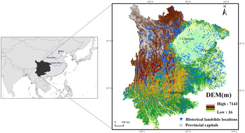
The selected study area is divided into a zone based on the geomorphological and geological zoning in a large number of existing studies (Wang et al. 2020b; Lin et al. 2021; Wang et al. 2021a; Lin et al. 2022). In terms of landforms, these areas have similar types of landforms, and the various landform forms are widely and evenly distributed in the region, which is also known as the Southwest Mountains within primary landform division of China (Wang et al. 2020b). Of these, lowland basins and plains, small undulating low mountains and small undulating middle mountains cover a large area and are mainly found in the Sichuan Basin, the Guizhou Plateau and the relatively low-lying areas of south-western Yunnan; canyon areas are mainly found in the Hengduan Mountains. In terms of geology, these areas are known as the Southwest Karst Rocky Mountain Geological Environment Zone, as they suffer from severe karst collapse and soil erosion. Geographically, the study area has a latitude and longitude range of 97°21′–110°11′ East and 21°8′–33°41′ North. The study area is approximately 1,123,000 square kilometres, one-ninth of the total area of China. The north-western part is high, and the south-eastern part is low, ranging from 16 m to 7143 m (Figure 1). The topography of the study area is steep, with an average slope of 17.3° and a maximum slope of 79.6°.

Figure 1. The location of the study area together with the spatial distribution of historical landslides.

Climatically, the southwest region consists mainly of a subtropical monsoon climate and a highland mountain climate. The average annual precipitation in the region is approximately 1,130 mm, with the rainy season generally occurring from July to September. Heavy torrential rainfall accounts for more than 50% of the total annual precipitation. The region is subject to monsoonal circulation and complex geography and often experiences heavy localized precipitation, making it one of the most varied and complex places in China in terms of localized regional differences in precipitation.

In summary, the southwest region is part of the eastern monsoon zone, with a humid climate and abundant precipitation; the undulating terrain greatly increases the effect of gravity, and in the event of heavy, or continuous, rainfall, it makes the rocks of the mountains lose, making landslides easy to occur.

2.2. Historical landslide inventory

The landslides utilized in this study are from the National Detailed Survey of Geological Hazards. Since 2005, the China Geological Survey has progressively conducted the detailed survey of six kinds of geological hazards, such as ground fractures, avalanches, landslides, ground subsidence, ground subsidence and debris flows. The most frequent type of landslide and the one that poses the most risk is the flow type landslide in the research area. This particular kind of landslide is distinguished by a significant vertical drop, rapid movement, a sizable volume, extraordinarily lengthy travel distances, and great mobility. For example, on 23 July 2019, a very large landslide occurred in Shuicheng County, Guizhou Province, in the study area. This landslide was initiated and scraped along 2 original alluvial ditches on the slope, expanding and accelerating, blocked by the raised terrain, partly accumulating in the upper and middle parts of the stacked slope, and the rest turning into a high-speed debris flow sliding down, impacting the slope settlement, involving a total of 23 households, 77 people and 27 houses, 21 of which were buried. Therefore, representative records of flow-type landslides caused by rainfall were chosen for susceptibility assessment. During that time, these landslides resulted in huge economic and personal losses. A total of 5,281 flow-type landslides caused by rainfall were applied to model landslide susceptibility. These landslides were plotted as vector points representing the center of the landslides’ mass. Each landslide record was provided with information about landslide type, geographic description, latitude and longitude, landslide cause as well as natural environmental conditions (Chen et al. 2019; Arabameri et al. 2021; Lin et al. 2021; Wang et al. 2022). The 5281 vector points were extracted using GIS technology. In addition, the mapping unit of this study was a 1 km spatial resolution grid. The spatial distribution of the historical landslide inventory is displayed in Figure 1.

2.3. Landslide conditioning factors

The critical step in landslide susceptibility modelling is the choice of proper landslide regulating factors. The environmental factors influencing landslide occurrence are concluded into 7 categories, that is, topographic factors, geological and soil factors, climatic factors, land cover factors, vegetation factors, hydrological factors and human activity factors (Reichenbach et al. 2018). According to the landslide features in the research area and previous researches, a total of 12 candidate moderators were taken into consideration from these 7 categories, namely mean annual precipitation, frequency over empirical rainfall threshold, lithology, soil type, soil moisture, slope, curvature, normalized vegetation cover index (NDVI), land use, road density, curve number (CN) and drainage density.

For the climatic factors, average annual precipitation was employed as a static environmental factor in order to characterize the spatial variability of precipitation features within the research area. Previous researches have indicated that the higher the mean annual precipitation, the higher the landslide sensitivity, and other affecting factors are similar. Similar variables have been utilized in current landslide researches (Arab Amiri and Conoscenti 2017; Lin et al. 2021). The mean annual precipitation (1981–2010) was estimated based on CN05.1 gridded data. The frequency of rainfall events above the empirical threshold proposed by Wang et al. (2021a) was calculated and used to represent the spatial heterogeneity of extreme precipitation.

For the geological and soil factors, the three indicators of lithology, soil type and soil moisture were chosen. It is well recognized that lithology has a great effect on the incidence of landslides, and changes in lithology often cause differences in the intensity and permeability of both and rocks (Huang et al. 2020; Orhan et al. 2022; Lin et al. 2021; Sahin 2022). There were 12 various lithological classes in the research area, as exhibited in Figure 2a. The lithology data were gathered from the novel global lithology map (Hartmann and Moosdorf 2012). The kind of soil on a slope influences the incidence of landslides (Orhan et al. 2022). Soil type affects the extent of damage, erosion and drainage, which in turn influences the landslide occurrence (Nhu et al. 2020). Soil type data were obtained from the RESDC. The soil types included nine categories, as shown in Figure 2f. Soil moisture can represent the average moisture condition of the soil. Compared to the average annual rainfall, it avoids interruptions of extreme rainfall, can reflect the possibility of long-term slope instability and can be used as a fundamental factor in the occurrence of landslides (Lin et al. 2017). It also has a substantial effect on large-scale landslides (Lin et al. 2021). The data of soil moisture derived from the dataset of Global High-Resolution Soil-Water Balance, involving the gridded estimates of actual evapotranspiration and soil water deficit (Trabucco and Zomer 2010). The index of soil moisture in this research is the annual mean soil water content as a percentage of the greatest soil water content in the period of evaporation.

Figure 2. Spatial distribution of landslide conditional factors. Lithology (MT: metamorphic rocks; PA: acid plutonic rocks; PB: basic plutonic rocks; PI: intermediate plutonic rocks; PY: pyroclastic rocks; SC: carbonate sedimentary rocks; SM: mixed sedimentary rocks; SS: siliciclastic sedimentary rocks; SU: unconsolidated sediments; VA: acid volcanic rocks; VB: basic volcanic rocks; VI: intermediate volcanic rocks). Soil type (10: lacustrine; 11: semi-lacustrine; 15: incipient; 16: semi-hydromorphic; 17: hydromorphic; 19: anthropogenic; 20: alpine; 21: ferro-aluminous; 23: rock). Land use (1: arable land; 2: forestland; 3: grassland; 5: urban and rural industrial and mining residential land; 6: unused land).

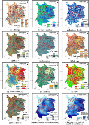
With regard to topographic factors, the two indicators chosen were slope and curvature. The slope is an important parameter in landslide susceptibility assessment. In areas with high and growing slope gradients, the landslide risk is elevated. Changes in slope gradient and deterioration of materials on slopes are the most important factors contributing to the occurrence of landslides (Sahin 2022). Slope gradient plays an important role in landslides and is thus frequently utilized for landslide susceptibility mapping (Huang et al. 2020; Lee et al. 2020; Orhan et al. 2022; Sahin 2022). In addition, curvature, which generally refers to the rate of change in slope or slope orientation, is believed to be one of the primary factors controlling the surface geometry of the terrain on which landslides occur (Sahin 2022). The curvature factor is a crucial parameter for the mapping of landslide susceptibility and gives information on topographic morphology (Orhan et al. 2022). The topographical data were derived from Shuttle Radar Topography Mission (SRTM) 90 m DEM (http://srtm.csi.odel.org). And the spatial resolution of the DEM was 90 m.

For the vegetation cover factor, the Normalized Difference Vegetation Index (NDVI) was chosen. NDVI is often thought to be a moderating factor in the modeling of landslide susceptibility as the root system of vegetation enhances slope stability and the extent of this consolidation determined by the particular features of the vegetation (Sahin 2022). Therefore, the effect of rainfall on hillsides can be alleviated through vegetation. NDVI is widely used to monitor the spatial distribution of physiological and biophysical characteristics of vegetation (Lee et al. 2020). In this study, NDVI data were obtained from RESDC.

Land use is a mixture of natural resources (e.g. soil, vegetation, water resources) and anthropogenic resources (e.g. places on the ground, roads, railways and buildings). The effects of land utilization change play a vital part in the research of environmental issues, particularly in evaluating the susceptibility of landslides (Orhan et al. 2022; Lin et al. 2021; Roccati et al. 2021; Sahin 2022). The land-use data used in this work were obtained from RESDC. The dataset was created using artificial visual interpretation of Landsat TM/ETM remote sensing photos from each epoch. The current land-use data from 2005 were chosen for this investigation due to the steady unfolding of geological disasters since 2005. Land use types can be divided into 5 categories in accordance with the first level, as illustrated in Figure 2h.

For the human activity, road density was chosen. Roads are usually the result of the action of human activity, and road density allows the impact of road works on the occurrence of landslides to be estimated (Chen et al. 2019). According to available studies, roads are a common location for landslides to occur, especially in mountainous areas (Shahabi and Hashim 2015). Furthermore, for the linear condition factors like roads, current researches primarily adopt the buffer analysis method in GIS to acquire discrete variables including road distance, which are stochastic and volatile and sensitive to the errors of the line or point elements, resulting in reduced accuracy in predicting landslide susceptibility, whereas the use of continuous conditioning factors such as road density can improve the applicability of linear factors as well as their clearer physical significance (Huang et al. 2022). In this study, road density data were obtained from RESDC.

For hydrological factors, the two indicators CN and drainage density were selected. CN is a comprehensive dimensionless parameter that characterizes the bottom ground surface prior to rainfall in a watershed and is used in hydrology to determine an approximation of the direct runoff volume for rainfall events in a given area. It is associated with pre-soil moisture, soil type, slope, land use, as well as other affecting factors, and is also extensively applied in the area of landslide susceptibility research (Hürlimann et al. 2022; Wang et al. 2022). Moreover, rivers can erode slopes or saturate the lower part of the material, thus negatively affecting stability until the water table rises (Orhan et al. 2022). The higher the drainage density, the greater the influence of river-cut slopes and the greater the likelihood of landslides occurring (Wang et al. 2022). Due to the large grid dimensions in this research, drainage density was utilized instead of the distance to the closest stream. In accordance with previous researches, the distance between slope and drainage line is an essential factor affecting slope stability, thus, drainage density is considered as an effective factor of landslide susceptibility by some researches (Zhao et al. 2018; Orhan et al. 2022; Wang et al. 2022). In this work, the data on drainage density were derived from the HydroSHEDS dataset (Linke et al. 2019), and the CN data were gathered from Zhao et al. (2018).

The source and basic information about all conditional factors are given in Table 1. The quantile classification method was adopted for all continuous variables including mean annual precipitation, frequency over empirical rainfall threshold, soil moisture, slope, curvature, NDVI, road density, CN, and drainage density. All the landslide conditional factors used in the study were resampled to 1 km spatial resolution.

Table 1. The sources of landslide conditional factors used in the study.

Category	Factors	Resolution	Data Type	Source
Climate data	Mean annual precipitation (1981–2010) (mm)	1km	GRID	National Meteorological Information Centre, China Meteorological Administration
	Frequency over empirical rainfall threshold (times/a)			Wang et al. (2021a)
Geological and soil data	Lithology	1km	GRID	Hartmann and Moosdorf (2012)
	Soil type			http://www.Resdc.cn
	Soil moisture (%)			Trabucco and Zomer (2010)
Topography data	Slope (°)	90 m	GRID	http://srtm.csi.odel.org
	Curvature
Vegetation cover data	NDVI	1km	GRID	http://www.Resdc.cn
Land cover and land use data	Land use	1km	GRID	http://www.resdc.cn
Human activity data	Road density	1km	GRID	http://www.resdc.cn
Hydrological data	Curve number	1km	GRID	Zhao et al. (2018)
	Drainage density			http://www.resdc.cn

3. Methods

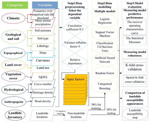
The methodological structure in this work is depicted schematically in Figure 3 and is divided into three key phases: data pre-processing, data modelling, and model evaluation. Firstly, 5281 non-landslide samples were randomly selected at a ratio of 1:1 in the non-landslide area based on the recommendations of previous studies. This was done because the result of the landslide susceptibility assessment is a binary classification problem, and both landslide and non-landslide samples should be used in order to better train the machine learning model (Orhan et al. 2022; Lin et al. 2021; Sahin 2022; Wang et al. 2022). In conjunction with the landslide samples, they constitute the dependent variable for the modelling of landslide susceptibility. In addition, several metrics were utilized to screen the influencing factor data, and the influences that were appropriate were employed as independent variables. We integrated the independent and dependent variables for the data modelling phase. Then 70% of the data were divided separately into the training set to train the model and 30% as the testing set to evaluate the model performance. In the stage of model assessment, many indicators were selected for the quantification and comparison of the model performance, and then the six models were employed in all of Southwest China to produce six landslide susceptibility maps. The geomorphological plausibility assessment was used to investigate the most reliable landslide susceptibility assessment model for Southwest China.

Figure 3. The main technical route performed in this study.

3.1. Selection of the dominate conditional factors

The selection of influencing variables as the final input for the data-driven landslide susceptibility model was on the basis of the spatial correlation, variance inflation factor (VIF) test and relative importance evaluation. To limit the problem of collinearity, all candidate variables were subjected to a Pearson correlation analysis to yield correlation coefficients, and variables with a strong correlation (correlation coefficient r > 0.7) were not selected for the model at the same time. Then, the spatial analysis function of ArcGIS was employed to construct a kernel density map of the historical landslides and a fishing net with a size of 1 × 1 km, and the mean kernel density, mean value of the continuous variables, and plurality of the categorical variables were tallied separately for each net. The VIF estimated by this multiple linear regression could distinguish the main influencing variables causing covariance, and it is generally considered that a VIF > 5 indicates a strong multifield covariance problem between independent variables, and such variables cannot be selected as input factors to the model at this time (O’brien 2007; Arabameri et al. 2021). The formula for calculating VIF is as follows: (1) $$\mathit{VIF}=\frac{1}{1-R_i^2}$$(1) where $R_i$ represents the negative correlation coefficient of the independent variable for the regression analysis of the remaining independent variables (O’brien 2007). Finally, the relative importance approach was utilized for filtering the relative correlation of the model’s input factors. The variable with the highest relative importance has the highest priority for each group of influencing factors.

3.2. Machine learning methods

3.2.1. Logistic regression (LR)

LR is based on dichotomous variables analysis (e.g. 0 and 1 or true and false) that are used to represent the outcome, which depends on one or more separated factors (Menard, 2002). Due to its principle simplicity and interpretability, the LR model has been extensively applied for exploring the mapping of landslide susceptibility (Lin et al. 2017; Lombardo and Mai 2018). The LR model is essentially a linear model. The principle can be given by the following formula: (2) $$P=\alpha +\sum _{k=1}^k{\beta }_k{x}_k\mathrm{ }$$(2) where P represents the dependent variable representing the absence (0) or presence (1), $\alpha$ is the model’ intercept, denotes the partial regression coefficients and represents the independent variables.

3.2.2. Support vector machine (SVM)

SVM is a multivariate nonlinear predictor with the benefits of global optimality and excellent generalization properties (Cortes and Vapnik 1995). SVM can be applied to linearly non-separable, high-dimensional data sets, and as such, it has been broadly and effectively employed in various regression and classification problems (Huang et al. 2020; Orhan et al. 2022). The properties of SVM are associated with its kernel functions, namely radial basis functions, polynomial and linear, sigmoid (Orhan et al. 2022). Among them, RBF is the most extensively adopted kernel. Therefore, in this study, RBF was used for modelling purposes.

3.2.3. Classification 5.0 decision trees (C5.0 DT)

In the family of decision trees, the Classification 4.5 decision tree (C4.5 DT) model is one of the most commonly utilized classification algorithms, while the classification 5.0 decision trees (C5.0 DT) is a modified version of C4.5 DT that which optimizes memory, simultaneously introduces the entropy concept (Saito et al. 2009). C5.0 DT can describe the structural patterns of relevant output and input variables efficiently with a tree architecture. In general, the construction of C5.0 DT involves the processes of tree growth, pruning of child nodes, facilitation of growth, and model closure. In comparison with other models, this model is easier to understand as the process of tree growth and removal can be well interpreted (Huang et al. 2020). In essence, C5.0 is an algorithm that evaluates the best partition according to the information gain ratio (IGR.) IGR is regarded as a probabilistic-based measure for computing the uncertainty reduction degree. Normally, the decision tree grows downward through the calculation of the partition with the largest IGR until the optimal solution is available. In this work, the C5.0 DT model parameters were set to default values.

3.2.4. Artificial neural network (ANN)

ANN model is a type of nonlinear classification technology. It is composed of a group of interconnected artificial neurons and possesses the ability to study the complex correlations between output and input variables (Fausett 2006). Artificial neural networks have a high degree of interpretability by simulating the process of data generation (Huang et al. 2020). In addition, characteristics in ANN have interdependent memory, self-learning, and independent statistical distributions (Phong et al. 2021).

The multilayer perceptron (MLP) neural network in ANN it is the most prevalent and extensively employed neural network architecture, composed of three layers: hidden layer, output layer and input layer. One of the hidden layers is designed to improve the networks ability to simulate complex functions (Paola and Schowengerdt 1995). Depending on the application, each layer in the net includes a sufficient amount of neurons. The input layer is a passive one, receiving only data (for example, data associated with a variety of causal factors). In contrast to the input layer, both the hidden layer and the output layer actively process the data. The output layer generates the outcome of the neural net. Backpropagation artificial neural nets are the most extensively utilized nets. The algorithm randomly chooses the initial weights of the inputs and employs the mean square error to conclude the difference between the expected and calculated values of all observation, iteratively repeating the BP algorithm until the network error reaches an acceptable value. Due to its high flexibility and adaptability in modelling, it is extensively employed in the researches of landslide susceptibility (Huang et al. 2020; Orhan et al. 2022). The ANN applied in this work composed of two output layers (landslide, non-landslide), a hidden layer (13 neurons) and an input layer (8 neurons), with all of other parameters (for instance learning rate set to default).

3.2.5. Random forest (RF)

An RF is a composition of tree predictions such that each tree is dependent on the value of a random vector that is individually sampled and has the identical distribution for all of the trees in the forest. As the tree population in the forest becomes larger, the forest generalization error converges to a limit RF is an aggregate machine learning technology that can build a large amount of decision trees to interpret the spatial relations of landslide occurrence (Kim et al. 2018). A forest of tree classifiers has a generalization error that is dependent on the intensity of the individual trees in the forest and the association between them (Breiman 2001). RF was first proposed in the literature as a useful tool for classification and regression problems as it combines decision trees with bagging and requires only a small number of parameters to be determined to obtain relatively good results (Naghibi et al. 2016; Orhan et al. 2022; Akinci and Zeybek 2021; Biçici and Zeybek 2021; Zeybek 2021; Aslam et al. 2022). For the construction of an RF model, the number of trees (ntree) and the input variables taken into account in each node partition must be specified (Orhan et al. 2022). In this study, the input variable by way of grid search was defined as 3 and ntree was defined as 550.

3.2.6. Categorical boosting (Catboost)

Categorical Boosting (Catboost) is a GBDT framework with fewer parameters, support for categorical variables and high accuracy based on a symmetric decision tree based learner, addressing the main pain point of efficient and rational processing of categorical features (Dorogush et al. 2018). In comparison to other machine learning models, the algorithm can deal with various data formats, like classification characteristics, and needs only a small amount of data for training. Moreover, Catboost solves the problem of Gradient Bias and Prediction shift, thus decreasing the occurrence of overfitting and thereby increasing the generality and precision of the algorithm (Sahin 2022).

Catboost has a total of 69 parameters, and due to its large number of parameters, it is quite difficult to find the optimal parameter team. Therefore, according to the foundation of previous researches, several important parameters in the model were mainly tuned in this study using random search, namely maximum tree depth for base learner (max_depth), depth of the tree (depth), boosting learning rate (learning rate), the frequency of iterations to calculate the values of objectives and metrics (metric_period) , the constant used to calculate the coefficient for multiplying the model on each iteration (model_shrink_rate rate) (Sahin 2022). In the end, max_depth, depth, learning rate, metric_period and model_shrink_rate were set to 5, 6, 0.03, 45 and 0.8, respectively, while all other parameters were set to default.

3.3. Model evaluation methods

In this work, eight quantitative metrics were applied to assess the predictive capability, reliability and operational efficiency of the model, namely AUC, ACC, F1, Kappa Index, RMSE, Heidke Skill Score (HSS), log loss and time to generate landslide susceptibility maps for the entire study area. The AUC derived using CV and SPCV was used to assess the robustness. The spatial distribution of landslide susceptibility maps was assessed qualitatively.

3.3.1. The receiver operating characteristics curve

The ROC curve is a technology extensively applied to determine the prediction ability and goodness of fit of probability models. The area under the curve (AUC) is utilized to assess the landslide model performance. AUC value ranging between 0 and 1, with values closer to 1 indicating better model performance, and values away from 1 suggesting worse performance. Based on previous researches, the model performance according to the AUC value can be classified as follows. 0.5-0.6 is poor, 0.6-0.7 is moderate, 0.7-0.8 is good, 0.8-0.9 is excellent, and 0.8-1 indicates almost perfect (Rahmati et al. 2017; Garosi et al. 2018).

3.3.2. Statistical measures

The statistical measures ACC, F1, and Kappa index are based on confusion matrices and are commonly employed in machine learning model evaluation. There are four quantities in the confusion matrix: TP, FP, TN, and FN. The description of these four quantities is given in detail in much of the literature (Huang et al. 2020; Orhan et al. 2022; Phong et al. 2021; Sahin 2022). The number of correct predictions as a percentage of the total is represented by ACC, and the ACC result is in the range of 0 to 1, where a value closer to 1 indicates higher accuracy. The formula for calculating ACC is as follows: (3) $$\mathit{ACC}=\frac{TN+TP}{TN+FN+FP+TP}$$(3)

F1 is the sum of accuracy and recall, and it has a range of 0 to 1, with a value closer to 1 indicating more accuracy and vice versa. The formula for calculating F1 is as follows: (4) $$F1=\frac{2\mathrm{*}TP}{2\mathrm{*}TP+FP+FN}$$(4)

Kappa index is a statistical measure of consistency. For classification problems, consistency is the agreement between the model predictions and the actual classification results. The kappa coefficient is calculated based on the confusion matrix and takes values between −1 and 1, with the closer to 1 the better the consistency. The formula for calculating Kappa index is as follows: (5) $$\mathit{Kappa}\mathrm{ }\mathit{inde}\mathrm{x}=\frac{\left(TP+TN\right)-\left[\right(TP+FN\left)\right(TP+FP)+(FP+FN\left)\right(FN+TN\left)\right]/(TP+FP+FN+TN)}{\left(TP+FP+FN+TN\right)-\left[\right(TP+FN\left)\right(TP+FP)+(FP+FN\left)\right(FN+TN\left)\right]/(TP+FP+FN+TN)}$$(5)

RMSE is a metric that measures the deviation between the observed and true values, and is one of the indicators of the outcome of the model predictions, with a smaller value indicating a positive fit of the model. The RMSE is calculated as follows: (6) $$\mathit{RMSE}=\sqrt{\sum _{i=1}^n\frac{{(zi-yi)}^2}{n}}\mathrm{ }$$(6) where $zi$ represents the actual value and $yi$ represents the predicted value.

HSS is also a statistical indicator whose practical significance is measured by the proportion of correct classifications after excluding those that are correct purely due to random chance, HSS is also named as Cohen’s kappa (Frattini et al. 2010). The formula for calculating the HSS is as follows: (7) $$\mathit{HSS}=\frac{2\mathrm{*}\left(TP\mathrm{*}TN\right)-\left(FP\mathrm{*}FN\right)}{\left(TP+FN\right)\mathrm{*}\left(FN+TN\right)+\left(TP+FP\right)\mathrm{*}(FP+TN)}\mathrm{ }$$(7)

Logarithmic loss (log loss) is another metric used for machine learning model performance evaluation and is formulated as follows: (8) $$\mathrm{Log}\mathrm{ }\mathit{loss}\mathrm{ }=\mathrm{ }-\frac{1}{M}\sum _{i=1}^M{y}_i\log \hspace{0.17em}\left(p\left(y_i=1\right)\right)+\left(1-y_i\right)\mathrm{l}\mathrm{og}(1-p(y_i=1\left)\right)$$(8) where $M$ represents the total sample number, $y_i$ represents the real label (1 or 0) of the ith sample, and $p\left(y_i=1\right)$ denotes the possibility that the predicted label of the ith sample is 1 (Wang et al. 2021b). The lower the log loss value is, the better the model performs in predicting landslide susceptibility (Wang et al. 2021b).

3.3.3. Robustness evaluation based on CV and SPCV

The model robustness can be confirmed through the CV and SPCV (Brenning 2012; Lin et al. 2021; Wang et al. 2022). Without respect to other parameters, the CV divides the original dataset into k sample sets at random, and the model is trained progressively by combining k-1 of them as the training dataset. The SPCV is a random division of the original dataset into k sample sets while accounting for spatial distribution. The k-1 combination was then applied as a training dataset for training the model.

All of the aforementioned experiments for the models were run on an I5-10300H 4-core processor running at 2.8 GHz with 16 GB of RAM, and all approaches were predominantly computed on the R language platform, which is an open-source statistical analysis software (version 4.1.1). The cor function and the corrplot package were used to generate the Pearson correlation coefficient, the carData package and the car package were used to implement stepwise regression, the relaimpo method in stepwise regression was used to implement relative importance ranking, and the VIF function was used to generate the VIF. In the data modelling phase of this study, LR was modelled mainly with the mgcv package, SVM was modelled mainly with the e1071 package, C5.0 DT was modelled mainly with the C50 package, ANN was modelled mainly with the nnet package, RF was modelled mainly with the Randomforest package, and Catboost was modelled using the Catboost package. The system.time() function was used to obtain the running time.

4 Results and discussion

4.1. Selection of candidate landslide influencing factors

Figure 4 and Table 2 present descriptive statistics for the candidate variables, including the Pearson correlation coefficient, VIF and relative importance of each candidate factor. As seen from the correlation coefficients in Figure 4 and the VIF in Table 2, there were no significant correlations (correlation coefficient < 0.7) or significant multicollinearity (VIF < 5) among the 12 candidate factors in this study (O’brien 2007). Further looking at the relative importance of the candidate variables in Table 2, four factors had a relative importance of less than 0.02, namely curvature, drainage density, mean annual precipitation and NDVI, thus these four factors were excluded. Eventually, the slope was selected as the topographic factor; the lithology, soil type and soil moisture were selected as the geological and soil factors; the land-use type was selected as the land cover factor; the CN was selected as the hydrological factor; the multiyear average frequency of precipitation exceeding the landslide sample threshold was selected as the meteorological and climatic factor; the road density was selected as the human activity factor, and all the above eight factors were included in the model as explanatory factors.

Figure 4. Pearson correlation coefficient among candidate affecting factors.

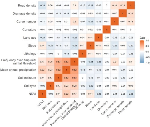
Table 2. The VIF and relative importance of candidate factors.

Candidate factor	VIF	Relative importance
Frequency over empirical rainfall threshold	2.857	0.139
Mean annual precipitation	2.576	0.016
Slope	1.934	0.368
Curve number	1.573	0.030
Land use	1.554	0.054
NDVI	1.549	0.009
Road density	1.387	0.035
Curvature	1.329	0.003
Soil moisture	1.309	0.157
Soil type	1.215	0.103
Drainage density	1.149	0.004
Lithology	1.084	0.083

4.2 Comparison of multiple machine learning models

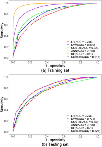
For predictive capability, the ROC curve is generally considered by the wise to be a relatively simple formula for assessing the accuracy of landslide susceptibility models, and the area under the ROC curve (AUC) is often used to assess the predictive performance of landslide susceptibility models (Rahmati et al. 2017; Garosi et al. 2018; Kim et al. 2018; Orhan et al. 2022; Arabameri et al. 2021). The ROC curves for each model on the training and testing sets are shown in Figure 5. Figure 5a reveals that in the training set, the AUC value of the RF model was the highest, and the curve was the steepest, followed by the Catboost model (AUC = 0.918). The other four models in descending order of AUC were the C5.0 DT model, SVM model, ANN model and LR model, with AUC values of 0.826, 0.809, 0.788, and 0.768, respectively. This result reveals that the Catboost model and RF model had outstanding predictive performance in the training set. This suggests that an ensemble model in the training set can fit the training set better, with nonlinear model having a moderate fit and linear model having a more limited fit. Nevertheless, the attributes of the training phase were not sufficient to assess the predictive power of the model, and the performance of the testing set was a better indicator of the generalisation performance of the model. According to Figure 5b, in the testing set, the optimum performer was the Catboost model (with AUC of 0.823), followed by the RF model (with AUC of 0.821), and the other four models in descending order of AUC were the SVM model, ANN model, LR model and C5.0 DT model, with AUC values of 0.775, 0.770, 0.756, and 0.751, respectively. The results in the testing set showed that all models showed varying degrees of decline in AUC values, but overall performance was consistent with the training set, with the ensemble model still far outperforming the linear and nonlinear models, followed by the nonlinear model and the single linear model with more limited performance. Based on the AUC, the linear model, the single nonlinear model, and the ensemble model all fit well (AUC > 0.7) in both the training and testing sets, with the ensemble model significantly outperforming the other models.

Figure 5. The ROC curves of the training and testing sets for different models.

It is not sufficient to validate the susceptibility map with a single ROC curve, as this may lead to inaccurate measurements if the samples are not evenly dispersed across the study area (Reichenbach et al. 2018; Arabameri et al. 2021). Therefore, in this study, various statistical indicators were used as alternative techniques to measure and compare the accuracy of the landslide susceptibility model as well as its reliability. Table 3 and Table 4 show the seven quantitative statistical metrics of the training and testing sets, namely, the ACC, F1, Kappa, RMSE, HSS, log loss and time taken to predict the whole study area. Of these, ACC, F1 based on confusion matrix and log loss based on loss function were used to further measure the predictive ability of the model; RMSE was used to measure the degree of model fit; Kappa and HSS were to measure the consistency of the model, and the time taken to predict the whole study area was to measure the operational efficiency of the model. Tables 3 and 4 give the statistical metrics for the training and testing sets, respectively.

Table 3. The statistical metrics in the training set of each model.

Model	ACC	F1	log loss	RMSE	Kappa	HSS
LR	0.698	0.694	0.576	0.443	0.501	0.441
SVM	0.731	0.734	0.537	0.423	0.558	0.499
C5.0 DT	0.762	0.764	0.508	0.409	0.622	0.553
ANN	0.709	0.722	0.566	0.441	0.505	0.463
RF	0.929	0.929	0.262	0.269	0.896	0.851
Catboost	0.837	0.839	0.393	0.351	0.753	0.687

Table 4 The statistical metrics in each model testing set and the running time.

Model	ACC	F1	log loss	RMSE	Kappa	HSS	Predict time (min)
LR	0.688	0.679	0.587	0.447	0.456	0.425	0.4
SVM	0.705	0.701	0.571	0.441	0.520	0.451	21.8
C5.0 DT	0.692	0.683	0.606	0.453	0.497	0.431	3.3
ANN	0.697	0.703	0.577	0.451	0.486	0.448	0.5
RF	0.740	0.738	0.517	0.418	0.582	0.516	1.6
Catboost	0.743	0.739	0.510	0.414	0.593	0.518	0.4

Table 3 shows that the model performances measured by the ACC, F1 and log loss metrics were relatively consistent in the training set, with the best performance from the RF model (ACC = 0.929; F1 = 0.929; log loss = 0.262), followed by the Catboost model (ACC = 0.837; F1 = 0.839; log loss = 0.393), and then the next four models were as follows: C5.0 DT model (ACC = 0.762; F1 = 0.764; log loss = 0.508), SVM model (ACC = 0.731; F1 = 0.734; log loss = 0.537), ANN model (ACC = 0.709; F1 = 0.722; log loss = 566), and LR model (ACC = 0.698; F1 = 0.694; log loss = 0.576). In contrast, the model performances of the ACC, F1 and log loss showed microscopic changes in the testing set. The models in bold in Table 4 were those that performed well. For the ACC, the optimum model was the Catboost model (ACC = 0.743), followed by the RF model, SVM model, ANN model, C5.0 DT model, and LR model, with ACC values of 0.740, 0.705, 0.697, 0.692, and 0.688, respectively. For F1, the best model was the Catboost model (F1 = 0.739), subsequently the RF model, SVM model, ANN model, C5.0 DT model, and LR model, with F1 values of 0.738, 0.701, 0.697, 0.683, and 0.679, respectively. In terms of log loss, the best was the Catboost model (log loss = 0.510), followed by the RF model (log loss = 0.517), the SVM model (log loss = 0.571), the ANN model (log loss = 0.577), the LR model (log loss = 0.587), and the C5.0 DT model (log loss = 0.606). Based on the aforementioned three statistical measures, it was demonstrated that the ensemble model’s overall sample was predicted more precisely than the other models in the training set and testing set, followed by the nonlinear model and then the linear model. The RMSE results also demonstrated that an ensemble model might obtain a higher goodness of fit.

Furthermore, the reliability of the landslide susceptibility models was assessed using Kappa and HSS, and the results showed that the RF model reaches much higher values in comparison with the other five models in the training set, with Kappa and HSS of 0.896 and 0.851, respectively, indicating that the RF model achieved almost high consistency; followed by the Catboost model with Kappa and HSS of 0.753 and 0.687, suggesting that the Catboost model achieves a high degree of consistency. The Kappa and HSS for the other four models were largely between 0.4 and 0.6, indicating a moderate degree of consistency between the linear and nonlinear models. In the testing set, the Kappa coefficients and HSS of all six models ranged between 0.4 and 0.6, with the highest values still being achieved by the two models using the tree as the baseline classifier.

Finally, the efficiency of the models was evaluated by calculating the time taken by each model for predicting the landslide susceptibility map for the entire study area, which in this study had a total of 2024088 pixels. The time taken to predict the entire study area was approximately the same and shortest for the LR model (predicted time = 0.4 min) and the Catboost model (predicted time = 0.4 min), followed by the ANN model (predicted time = 0.5 min), the RF model (predicted time = 1.6 min), the C5.0 DT model (predicted time = 3.3 min), and the longest time was for the SVM model (predicted time = 21.8 min). Since gradient boosting models with tree-based classifiers, like the Catboost model, also achieve faster run efficiencies, this result suggests that ensemble models are also superior in terms of run efficiency. The single linear model appears to have the fastest computational power, most likely as a result of its simpler principle.

Additionally, the AUC of each model was determined independently using the CV and SPCV methods on 30% different test sets in order to further evaluate the robustness of the prediction capacity of the models on non-spatial and spatial subsets. In the experiments, the CV and SPCV procedures were applied 250 times, fivefold 50 times for each model. Table 5 shows the median and upper and lower quartiles of the total 250 AUC values obtained in the testing set by CV and SPCV. In the CV results for each model, the median AUC for the six models ranged from 0.707 to 0.804, with the median for the Catboost and RF models being 0.804 and 0.803, respectively. This result indicates that all six models, especially the RF and Catboost models, distinguished well between non-landslide samples and landslide samples. While looking at the upper and lower quartile distances, the ANN model reached a place difference of 0.08, and none of the other five models except the ANN model had a place difference in CV greater than 0.02. This result indicates the poor robustness of the ANN model, while the other five models performed fairly consistently on the multiple random test datasets. The median AUC of each model in SPCV results ranged from 0.566 to 0.714, with varying degrees of decline compared to CV, with the RF and Catboost models, which performed better in general cross-validation, having median values of 0.688 and 0.653, respectively, and the LR model, which performed moderately well in general cross-validation, performing best. This result demonstrates that the six models performed well in SPCV, with the LR model outperforming the others. When comparing the upper and lower SPCV interquartile distances of the models, all models showed a tendency to widen their interquartile distances compared to CV, with the five models except the SVM model having interquartile distances between 0.1 and 0.2, while the SVM with the lowest median value performed more consistently in SPCV with an interquartile distance of less than 0.1. This result suggests that the ensemble model was the most robust without considering the spatial distribution of the landslide samples, while the linear model was able to show the highest robustness when the spatial distribution was considered.

Table 5. Performance of the cross-validations in the testing set.

Model	The AUC of CV	The AUC of SPCV
	Median (1st-3rd quantile)	Median (1st-3rd quantile)
LR	0.747 (0.740–0.757)	0.714 (0.630–0.766)
SVM	0.707 (0.701–0.708)	0.566 (0.541–0.612)
C5.0 DT	0.738 (0.723–0.732)	0.671 (0.549–0.724)
ANN	0.716 (0.673–0.754)	0.629 (0.579–0.688)
RF	0.803 (0.796–0.807)	0.688 (0.632–0.779)
Catboost	0.804 (0.795–0.814)	0.653 (0.595–0.785)

4.3. Comparison of the spatial appearances of landslide susceptibility maps

Each created landslide susceptibility model was used for the whole research area, and then a landslide susceptibility probability map was derived from each of the models. The probability values ranged from 0 and 1. The closer the value was to 1, the higher the landslide probability was, while values closer to zero indicated a landslide was less likely to occur. Because the model in this research was created utilizing non-landslide and landslide data with a 1:1 ratio, the probability value of landslide susceptibility predicted via the model should be relative. Namely, the landslide susceptibility should be relatively low and relatively high (Lin et al. 2021). In addition, if a natural break in data classification is proposed, a very high susceptibility category will dominate the entire map (Sahin 2022). As a result, in this work, the relative quantile approach was employed for classifying the landslide susceptibility values calculated by each model into five categories, which represented the susceptibility classes of landslide occurrence (Lin et al. 2021; Sahin 2022; Wang et al. 2022). The classification was based on the probability values corresponding to the 20th, 40%, 60% and 80% percentiles of the predicted landslide susceptibility values corresponding to the extremely low, low, medium, high and extremely high susceptibility levels, respectively (Sahin 2022; Lin et al. 2021; Wang et al. 2022).

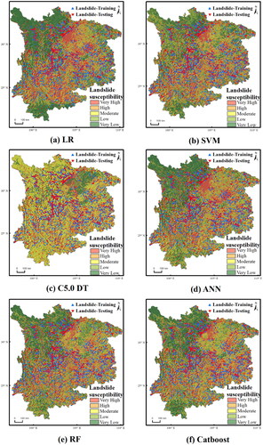
Figure 6(a–f) shows the spatial distribution of landslide susceptibility. When the susceptibility maps generated by all the models were visually analysed, the Sichuan Basin and high elevations were frequently where the research area’s extremely high and high susceptibility zones were found. Low and very low landslide susceptibility zones are primarily located in the north-western part of the research area and also correspond more closely in spatial distribution to the historical landslide sample sites, so it can be concluded that all the landslide susceptibility maps created from the model were successful. However, the geographic maps of landslide susceptibility generated by the various models still showed some regional heterogeneity and implausibility. The LR model (Figure 6a) depicted areas of extremely high susceptibility, primarily in mountainous areas, but they were also found in continuous patches in central Sichuan and central Guizhou and in isolated locations in Southeast China to a lesser extent. When the spatial distribution characteristics of road density in the southwest (Figure 2j) were combined with the historical landslide distribution characteristics, it was clear that the susceptibility probability maps drawn by the LR model contained some irrationalities, with urban areas with high road density also being classified as very highly susceptible areas. In comparison to the LR model, the SVM model (Figure 6b) depicted areas of very high susceptibility that were more discrete, with only a continuous block distribution in central Chengdu, but still with considerable implausibility. The C5.0 DT model (Figure 6c) mapped areas of very high susceptibility, primarily in mountainous areas and less in non-mountainous areas, which was somewhat inconsistent with the historical distribution of landslide samples. Furthermore, in the susceptibility probability map of this model, the probability of susceptibility was moderate in most regions. When the spatial distribution characteristics of the topographic slope in the southwest (Figure 2d) were combined with the spatial distribution of historical landslide samples, it was somewhat implausible that the northwest, which has a gentle slope and almost no historical landslide samples, was also classified as moderately probable. The ANN model (Figure 6d) depicted areas of extremely high susceptibility that were more similar to the LR model (Figure 6a) and had the same issues. The RF model landslide susceptibility map (Figure 6e) and the Catboost landslide susceptibility map (Figure 6f) had more consistent spatial distribution characteristics and thus better simulated the spatial distribution of landslides in historically high- and low-susceptibility areas and the RF model could better simulate the actual spatial distribution in central Sichuan than could the Catboost model. This result showed that, based on geomorphological knowledge, the ensemble model with a tree as the baseline classifier generated a more plausible map of landslide susceptibility than those generated by a single linear model and a single nonlinear model.

Figure 6. Spatial distribution of landslide susceptibility.

However, since the distribution of magnetization rates varies from region to region, it is highly arbitrary to rely judgments on geomorphological knowledge alone. Due to this, the resulting landslide susceptibility map’s percentage of historical landslide samples inside each susceptibility class was also calculated, as shown in Figure 7a. The findings demonstrate that none of the six models’ simulations of historical landslide samples in the very low susceptibility zone exceeded 2%. The Catboost model had a value of 73%, the RF model had an 81% percentage of very high susceptibility level, and the other four models had values of 50–60%. With the RF model producing the best results for the occupied areas of actual landslide sites, followed by the Catboost model, this result demonstrates that all three types of models had good practical simulations. This finding also suggests that the landslide susceptibility maps generated from the ensemble model more accurately model the distribution of historical landslide samples.

Figure 7. The percentage of landslide samples and non-landslide samples within each susceptibility level.

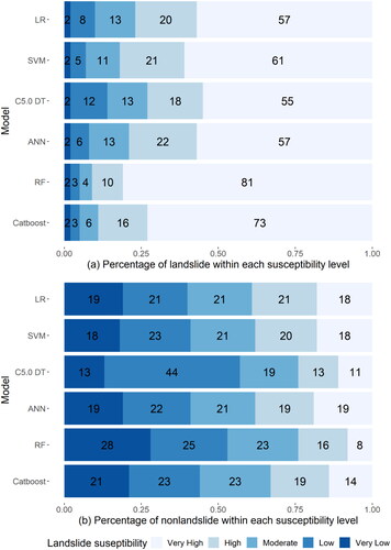
In addition, because the model developed in this paper was based on 1:1 ratio of landslide to non-landslide samples, i.e. the percentage of randomly produced non-landslide samples in each susceptibility class, as well as the percentage of historical landslide samples in each susceptibility level, were calculated, as shown in Figure 7b. For the non-landslide samples within the high and vary high levels of susceptibility, the RF and C5.0 DT models had superior performance to the other models, follow by the Catboost model, with the remaining three models reproducing comparable results. In contrast, at low and very low levels of susceptibility, the C5.0 DT model possessed the optimum simulation effect on non-landslide samples, followed by the RF model, with the other four models being more similar. This result suggests that the model with the best landslide sample simulation does not necessarily have the best non-landslide sample simulation; for example, the actual spatial distribution of the C5.0 DT model in the current work does not match the landscape, and its historical landslide sample simulation is average, but its effect on the non-landslide sample simulation is optimal, which may be related to its principle and data structure, so the model should be used with more caution in generating predictions (Steger et al. 2017; Lin et al. 2021). Overall, the ensemble model has better simulation results for both landslide and non-landslide samples created at a 1:1 ratio than the other two models, and thus the resulting landslide susceptibility maps have higher practical application value.

Machine learning models have recently received much attention in landslide susceptibility research as they are more accurate than other quantitative models used in the field, such as heuristic and traditional statistical models (Huang et al. 2020). However, there are numerous types of machine learning models, and it remains controversial which models have the most reliable prediction accuracy (Steger et al. 2017; Chen et al. 2019; Huang et al. 2020; Lin et al. 2021). In response, this paper selects linear, nonlinear and ensemble models widely used for landslide susceptibility modelling for a comparative study to further explore more reliable landslide susceptibility maps. The findings of this study demonstrate that ensemble models with tree classifiers outperform nonlinear and linear models in terms of predictive power, fit, reliability, and running efficiency on both the training and test sets, with the Caboost model outperforming the RF model. This is largely consistent with previous research, which showed that ensemble models typically perform better in terms of prediction than linear and nonlinear models (Akinci and Zeybek 2021; Youssef and Pourghasemi 2021; Hassangavyar et al. 2022; Hussain et al. 2022; Kavzoglu and Teke 2022; Orhan et al. 2022; Sahin 2022; Sarwar et al. 2022; Ye et al. 2022). The newer gradient ensemble approach does, though, appear to have a lot of value for the study of landslide susceptibility (Sahin 2022; Ye et al. 2022). Furthermore, the results of this paper show that the predictive performance of the three nonlinear models is relatively close, with the SVM slightly outperforming the ANN and C5.0 DT models, a performance similar to the former, but in another performance, the ANN and C5.0 DT achieved better results than the SVM (Naghibi et al. 2016; Xiong et al. 2020; Phong et al. 2021; Aslam et al. 2022; Orhan et al. 2022). There are also relevant studies that show that C5.0 DT has the highest predictive performance (Huang et al. 2020; Miao et al. 2022; Sheng et al. 2022). It may be related to their different data structures and the factors chosen to influence them. On the other hand, the single linear model may operate most efficiently due to its simple structure, but its corresponding predictive power is also more limited. On this basis, the robustness of the models were further assessed by applying CV and SPCV. The results of this study show that ensemble models with high predictive performance (i.e. tree-based classifiers) are also usually the most robust when spatial correlation is not considered, while single linear models achieve the highest robustness when spatial autocorrelation is considered (i.e. when the spatial distribution of landslide sample points is not homogeneous). This result suggests that no model is the best in every situation and for every metric. Each model has its strengths and limitations. In addition, further qualitative assessment of the generated landslide susceptibility maps produced results that were more similar to the quantitative test indicators, but there were some spatial differences; for example, the C5.0 DT and LR models in this study had fairly close indicator values in the testing set, but their actual geographical distribution was significantly different, even for models with relatively close predictive accuracy in the testing set. When conducting landslide susceptibility assessment studies, it is necessary to combine various elements and indicators to quantitatively assess the performance of the models, rather than relying on just one to quantify the model performance. In order to establish the best model, it is also necessary to carry out a qualitative analysis of landslide susceptibility mapping in order to validate the results of the quantitative assessment. This might be because, as mentioned in the review, models with high statistical values outperform those with low statistical values, but from a geomorphological standpoint, the second model might be more meaningful (reliable and useful) than the first because it might account for local conditions or pertinent geomorphological features (Reichenbach et al. 2018).

4.4. Ranking of the influencing factors

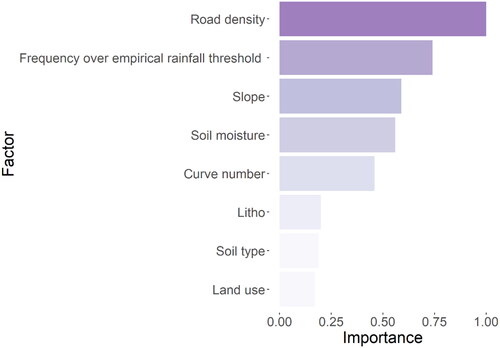
In this paper, the RF model was selected to explore the significance of input variables because it has higher prediction accuracy and simulation outcomes than the other models. The Gini index is an indicator that splits a given factor and gives the importance of the factor. When the average decline in the Gini index for a given split factor is greater, the split factor is more important (Xiong et al. 2020). The Gini index is frequently used to estimate the value of total variance in classification issues, and it is well suited for analysing the relevance of the input factors in this study; thus, this work also used the RF model and the Gini index to evaluate factor importance. Figure 8 displays the relative importance of each factor applied to the Gini index in the RF model, the outcomes of which are expressed relative to the maximum value, and overall, all eight factors were explanatory factors for landslide susceptibility. Of these eight factors, the larger average decreases in the Gini index were in road density, frequency over empirical rainfall threshold, slope, soil moisture and CN, with smaller decreases in lithology, soil type and land-use type. This result suggests that human-caused road density is the dominant factor in Southwest China and that topography, precipitation, and hydrology are all important triggers, which is consistent with previous research on the most important influencing factors (Wang et al. 2021c; Hassangavyar et al. 2022; Sahin 2022; Wang et al. 2022).

Figure 8. The relative significance of each factor in the Gini index-based RF model.

However, the model accuracy acquired in this paper is unsatisfactory, and there are numerous reasons for this, some of which may be related to the dataset utilized for the landslide influence factor’s poor resolution. The results of Arabameri et al. (2019) implied that different DEMs with different spatial resolution data sources might possess a considerable effect on the model’ accuracy. Furthermore, Reichenbach et al. (2014) observed that landslide susceptibility changed from 1954 to 2009 due to anthropogenically driven land-use change in northern Sicily, Italy. More importantly, within the time framework of modern climate projections (i.e. from decades to centuries), landslide sensitivity may vary as a result of meteorological and environmental variations constrained or driven through projected climate change (Reichenbach et al. 2018). In response, some academics have tried to consider potential future climatic scenarios and have performed susceptibility analyses in recent years (Kim et al. 2015). But it is unknown how various spatial and temporal scales of human activity and climate change may affect landslide susceptibility. As a result, further research is required to fully understand the results of models that use DEMs with different resolutions, account for more human activity, and incorporate future climate models.

5. Conclusion

The purpose of this research is to compare three machine learning models for the prediction of landslide susceptibility, i. e. a single linear model (represented by the LR model), a single nonlinear model (represented by the SVM model, C5.0 DT model and ANN model) and an ensemble model with the tree as the baseline classifier (represented by the RF model and Catboost model), to explore the common data-driven models for landslide susceptibility prediction performance and further generate more reasonable landslide susceptibility maps. Southwest China was selected as the study area with 5281 landslides causing significant impacts were recorded. Firstly, landslide impact factors in the region were screened based on three indicators: correlation coefficient, VIF and relative importance. The model was then constructed and ROC curves, and six quantitative statistical indicators (including ACC, F1, log loss, RMSE, Kappa and HSS) were applied for investigating the reliability and predictive power of the model. In addition, CV and SPCV were used to explore the robustness of the model on non-spatial and spatial subsets. For producing the landslide susceptibility maps, the model was ultimately applied to the full research region. With an aim of assessing the spatial distribution of the actual landslide susceptibility maps, a qualitative method on the basis of expert experience was applied. Finally, causal analysis was performed using the identified optimal model. These summaries can be acquired: (1) Ensemble models are more suitable for landslide susceptibility prediction as they have higher predictive performance and more reasonable spatial distribution than linear and nonlinear models. (2) For model robustness, the three types of models in CV performed relatively similarly in terms of predictive power, while in SPCV, the linear model LR (median AUC = 0.714) achieved better results than the ensemble and nonlinear models, a result that suggests that linear models may have the best robustness when the landslide sample point space is not homogeneous. It may not be sufficient to rely on one indicator alone for optimal model selection; it is best to consider multiple indicators from multiple sources, combined with appropriate knowledge of geomorphology. (3) Human activity factors, represented by road density, are the dominant factors in the frequency of landslides in Southwest China.

Disclosure statement

No potential conflict of interest was reported by the author(s)

Data availability statement

The data used in this work are available from the corresponding author on reasonable request.

References

- Ahmadlou M, Ebrahimian Ghajari Y, Karimi M. 2022. Enhanced classification and regression tree (CART) by genetic algorithm (GA) and grid search (GS) for flood susceptibility mapping and assessment. Geocarto Int. :1–20.
- Akinci H, Zeybek M. 2021. Comparing classical statistic and machine learning models in landslide susceptibility mapping in Ardanuc (Artvin). Nat Hazards. 108(2):1515–1543.
- Arab Amiri M, Conoscenti C. 2017. Landslide susceptibility mapping using precipitation data, Mazandaran Province, north of Iran. Nat Hazards. 89(1):255–273.
- Arabameri A, Chandra Pal S, Rezaie F, Chakrabortty R, Saha A, Blaschke T, Napoli D, Ghorbanzadeh O, Thi Ngo PT. 2021. Decision tree based ensemble machine learning approaches for landslide susceptibility mapping. Geocarto Int. 37(16):1–35.
- Arabameri A, Pradhan B, Lombardo L. 2019. Comparative assessment using boosted regression trees, binary logistic regression, frequency ratio and numerical risk factor for gully erosion susceptibility modelling. Catena. 183:104223.
- Aslam B, Zafar A, Khalil U. 2022. Comparison of multiple conventional and unconventional machine learning models for landslide susceptibility mapping of Northern part of Pakistan. Environ Dev Sustain. :1–28.
- Biçici S, Zeybek M. 2021. Effectiveness of training sample and features for random forest on road extraction from unmanned aerial vehicle-based point cloud. Transp Res Rec. 2675(12):401–418.
- Breiman L. 2001. Random forests. Machine Learning. 45(1):5–32.
- Brenning A. 2012. Spatial cross-validation and bootstrap for the assessment of prediction rules in remote sensing: the R package sperrorest. In 2012 IEEE International Geoscience and Remote Sensing Symposium. IEEE; p. 5372–5375..
- Centre for Research on the Epidemiology of Disasters–CRED. 2022. EM-DAT: the International Disaster Database [accessed 15 February 2022]. https://public.emdat.be/data/.
- Chen W, Panahi M, Tsangaratos P, Shahabi H, Ilia I, Panahi S, Li S, Jaafari A, Ahmad BB. 2019. Applying population-based evolutionary algorithms and a neuro-fuzzy system for modeling landslide susceptibility. Catena. 172:212–231.
- Cortes C, Vapnik V. 1995. Support-vector networks. Mach Learn. 20(3):273–297.
- Dietterich TG. 2000. Ensemble methods in machine learning. In International workshop on multiple classifier systems. Berlin: Springer; p. 1–15.
- Dorogush AV, Ershov V, Gulin A. 2018. CatBoost: gradient boosting with categorical features support. arXiv Preprint arXiv. doi:10.48550/arXiv.1810.11363.
- Fausett LV. 2006. Fundamentals of neural networks: architectures, algorithms and applications. India: Pearson Education India.
- Frattini P, Crosta G, Carrara A. 2010. Techniques for evaluating the performance of landslide susceptibility models. Eng Geol. 111(1-4):62–72.
- Froude MJ, Petley DN. 2018. Global fatal landslide occurrence from 2004 to 2016. Nat Hazards Earth Syst Sci. 18(8):2161–2181.
- Garosi Y, Sheklabadi M, Pourghasemi HR, Besalatpour AA, Conoscenti C, Van Oost K. 2018. Comparison of differences in resolution and sources of controlling factors for gully erosion susceptibility mapping. Geoderma. 330:65–78.
- Haque U, Da Silva PF, Devoli G, Pilz J, Zhao B, Khaloua A, Wilopo W, Andersen P, Lu P, Lee J, et al. 2019. The human cost of global warming: deadly landslides and their triggers (1995–2014). Sci Total Environ. 682:673–684.
- Hartmann J, Moosdorf N. 2012. The new global lithological map database GLiM: a representation of rock properties at the Earth surface. Geochem Geophys Geosyst. 13(12). doi:10.1029/2012GC004370
- Hassangavyar MB, Damaneh HE, Pham QB, Linh NTT, Tiefenbacher J, Bach QV. 2022. Evaluation of re-sampling methods on performance of machine learning models to predict landslide susceptibility. Geocarto Int. 37(10):2772–2794.
- Huang F, Cao Z, Guo J, Jiang SH, Li S, Guo Z. 2020. Comparisons of heuristic, general statistical and machine learning models for landslide susceptibility prediction and mapping. Catena. 191:104580.
- Huang CM, Lee CT, Jian LX, Wei LW, Chu WC, Lin HH. 2022. Using fuzzy neural networks to model landslide susceptibility at the Shihmen Reservoir catchment in Taiwan. Water. 14(8):1196.
- Hürlimann M, Guo Z, Puig-Polo C, Medina V. 2022. Impacts of future climate and land cover changes on landslide susceptibility: regional scale modelling in the Val d’Aran region (Pyrenees, Spain). Landslides. 19(1):99–118.
- Hussain MA, Chen Z, Kalsoom I, Asghar A, Shoaib M. 2022. Landslide susceptibility mapping using machine learning algorithm: a case study along Karakoram highway (KKH), Pakistan. J Indian Soc Remote Sens. 50(5):849–866.
- IPCC. 2022. Climate change 2022: impacts, adaptation, and vulnerability. Contribution of Working Group II to the Sixth Assessment Report of the Intergovernmental Panel on Climate Change [H.-O. Pörtner, D.C. Roberts, M. Tignor, E.S. Poloczanska, K. Mintenbeck, A. Alegría, M. Craig, S. Langsdorf, S. Löschke, V. Möller, A. Okem, B. Rama (eds.)]. UK: Cambridge University Press. In Press.
- Kaiser M, Günnemann S, Disse M. 2022. Regional-scale prediction of pluvial and flash flood susceptible areas using tree-based classifiers. J Hydrol. 612:128088.
- Kavzoglu T, Teke A. 2022. Predictive Performances of ensemble machine learning algorithms in landslide susceptibility mapping using random forest, extreme gradient boosting (XGBoost) and natural gradient boosting (NGBoost). Arab J Sci Eng. 47(6):7367–7385.
- Kim JC, Lee S, Jung HS, Lee S. 2018. Landslide susceptibility mapping using random forest and boosted tree models in Pyeong-Chang. Korea. Geocarto Int. 33(9):1000–1015.
- Kim HG, Lee DK, Park C, Kil S, Son Y, Park JH. 2015. Evaluating landslide hazards using RCP 4.5 and 8.5 scenarios. Environ Earth Sci. 73(3):1385–1400.
- Kotsiantis SB, Zaharakis I, Pintelas P. 2007. Supervised machine learning: a review of classification techniques. Emerging Artificial Intelligence Applications in Computer Engineering. 160(1):3–24.
- Lee S, Lee MJ, Jung HS, Lee S. 2020. Landslide susceptibility mapping using Naïve Bayes and Bayesian network models in Umyeonsan, Korea. Geocarto Int. 35(15):1665–1679.
- Linke S, Lehner B, Ouellet Dallaire C, Ariwi J, Grill G, Anand M, Beames P, Burchard-Levine V, Maxwell S, Moidu H, et al. 2019. Global hydro-environmental sub-basin and river reach characteristics at high spatial resolution. Sci Data. 6(1):1–15.
- Lin Q, Lima P, Steger S, Glade T, Jiang T, Zhang J, Liu TX, Wang Y. 2021. National-scale data-driven rainfall induced landslide susceptibility mapping for China by accounting for incomplete landslide data. Geosci Front. 12(6):101248.
- Lin Q, Steger S, Pittore M, Zhang J, Wang L, Jiang T, Wang Y. 2022. Evaluation of potential changes in landslide susceptibility and landslide occurrence frequency in China under climate change. Sci Total Environ. 850:158049.
- Lin Q, Wang Y. 2018. Spatial and temporal analysis of a fatal landslide inventory in China from 1950 to 2016. Landslides. 15(12):2357–2372.
- Lin Q, Wang Y, Liu T, Zhu Y, Sui Q. 2017. The vulnerability of people to landslides: a case study on the relationship between the casualties and volume of landslides in China. Int J Environ Res Public Health 14(2):212.
- Lombardo L, Mai PM. 2018. Presenting logistic regression-based landslide susceptibility results. Eng Geol. 244:14–24.
- Mehrabi M. 2022. Landslide susceptibility zonation using statistical and machine learning approaches in Northern Lecco, Italy. Nat Hazards. 111(1):901–937.
- Merghadi A, Yunus AP, Dou J, Whiteley J, ThaiPham B, Bui DT, Avtar R, Abderrahmane B. 2020. Machine learning methods for landslide susceptibility studies: a comparative overview of algorithm performance. Earth Sci Rev. 207:103225.
- Miao F, Zhao F, Wu Y, Li L, Török Á. 2022. Landslide susceptibility mapping in three gorges reservoir area based on GIS and boosting decision tree model. doi:10.21203/rs.3.rs-1838482/v1.
- Naghibi SA, Pourghasemi HR, Dixon B. 2016. GIS-based groundwater potential mapping using boosted regression tree, classification and regression tree, and random forest machine learning models in Iran. Environ Monit Assess. 188(1):1–27.
- National Bureau of Statistics of China. 2021. China statistical yearbook 2021. China: China Statistics Press.
- Nhu VH, Hoang ND, Nguyen H, Ngo PTT, Bui TT, Hoa PV, Samui P, Bui DT. 2020. Effectiveness assessment of Keras based deep learning with different robust optimization algorithms for shallow landslide susceptibility mapping at tropical area. Catena. 188:104458.
- O’brien RM. 2007. A caution regarding rules of thumb for variance inflation factors. Qual Quant. 41(5):673–690.
- Orhan O, Bilgilioglu SS, Kaya Z, Ozcan AK, Bilgilioglu H. 2020. Assessing and mapping landslide susceptibility using different machine learning methods. Geocarto Int. 37(10):2795–2820.
- Paola JD, Schowengerdt RA. 1995. A detailed comparison of backpropagation neural network and maximum-likelihood classifiers for urban land use classification. IEEE Trans Geosci Remote Sens. 33(4):981–996.
- Petley D. 2012. Global patterns of loss of life from landslides. Geology. 40(10):927–930.
- Phong TV, Phan TT, Prakash I, Singh SK, Shirzadi A, Chapi K, Ly H, Ho LS, Quoc NK, Pham BT. 2021. Landslide susceptibility modeling using different artificial intelligence methods: a case study at Muong Lay district, Vietnam. Geocarto Int. 36(15):1685–1708.
- Rahmati O, Tahmasebipour N, Haghizadeh A, Pourghasemi HR, Feizizadeh B. 2017. Evaluation of different machine learning models for predicting and mapping the susceptibility of gully erosion. Geomorphology. 298:118–137.
- Reichenbach P, Busca C, Mondini AC, Rossi M, 2014. The influence of land use change on landslide susceptibility zonation: the Briga catchment test site (Messina, Italy). Environ Manage. 54(6):1372–1384.
- Reichenbach P, Rossi M, Malamud BD, Mihir M, Guzzetti F. 2018. A review of statistically-based landslide susceptibility models. Earth Sci Rev. 180:60–91.
- Roccati A, Paliaga G, Luino F, Faccini F, Turconi L. 2021. GIS-based landslide susceptibility mapping for land use planning and risk assessment. Land. 10(2):162.
- Sadiki M, Aghad M, Batchi M, Al Karkouri J. 2022. Landslide susceptibility mapping using machine learning techniques and comparison of their performance at Ziz upper watershed, Southeastern Morocco. doi:10.21203/rs.3.rs-1534262/v1
- Sahin EK. 2022. Comparative analysis of gradient boosting algorithms for landslide susceptibility mapping. Geocarto Int. 37(9):2441–2465.
- Saito H, Nakayama D, Matsuyama H. 2009. Comparison of landslide susceptibility based on a decision-tree model and actual landslide occurrence: the Akaishi Mountains, Japan. Geomorphology. 109(3-4):108–121.
- Sarwar MS, Fatima SA, Aman M, Shoaib A, Aslam B, Zafar A. 2022. Landslide susceptibility mapping for Muzaffarabad region using machine learning algorithms. doi:10.21203/rs.3.rs-1504882/v1.
- Shahabi H, Hashim M. 2015. Landslide susceptibility mapping using GIS-based statistical models and Remote sensing data in tropical environment. Sci Rep. 5(1):1–15.
- Sheng M, Zhou J, Chen X, Teng Y, Hong A, Liu G. 2022. Landslide susceptibility prediction based on frequency ratio method and C5.0 decision tree model. Front Earth Sci. 10:918386.
- Steger S, Brenning A, Bell R, Glade T. 2017. The influence of systematically incomplete shallow landslide inventories on statistical susceptibility models and suggestions for improvements. Landslides. 14(5):1767–1781.
- Trabucco A, Zomer RJ. 2010. Global soil water balance geospatial database. CGIAR Consortium for Spatial Information. http://www.cgiar-csi.org
- Wang G, Chen X, Chen W. 2020a. Spatial prediction of landslide susceptibility based on GIS and discriminant functions. Int J Geoinf. 9(3):144.
- Wang N, Cheng W, Wang B, Liu Q, Zhou C. 2020b. Geomorphological regionalization theory system and division methodology of China. J Geogr Sci. 30(2):212–232.
- Wang D, Hao M, Chen S, Meng Z, Jiang D, Ding F. 2021c. Assessment of landslide susceptibility and risk factors in China. Nat Hazards. 108(3):3045–3059.
- Wang C, Lin Q, Wang L, Jiang T, Su B, Wang Y, Mondal S, Huang J, Wang Y. 2022. The influences of the spatial extent selection for non-landslide samples on statistical-based landslide susceptibility modelling: a case study of Anhui Province in China. Nat Hazards. 112(3):1967–1988.
- Wang N, Lombardo L, Gariano SL, Cheng W, Liu C, Xiong J, Wang R. 2021a. Using satellite rainfall products to assess the triggering conditions for hydro-morphological processes in different geomorphological settings in China. Int J Appl Earth Obs Geoinf. 102:102350.
- Wang H, Zhang L, Luo H, He J, Cheung RWM. 2021b. AI-powered landslide susceptibility assessment in Hong Kong. Eng Geol. 288:106103.
- Xiong K, Adhikari BR, Stamatopoulos CA, Zhan Y, Wu S, Dong Z, Di B. 2020. Comparison of different machine learning methods for debris flow susceptibility mapping: a case study in the Sichuan Province, China. Remote Sens. 12(2):295.
- Ye P, Yu B, Chen W, Liu K, Ye L. 2022. Rainfall-induced landslide susceptibility mapping using machine learning algorithms and comparison of their performance in Hilly area of Fujian Province, China. Nat Hazards. 113(2):965–995.
- Youssef AM, Pourghasemi HR. 2021. Landslide susceptibility mapping using machine learning algorithms and comparison of their performance at Abha Basin, Asir Region, Saudi Arabia. Geosci Front. 12(2):639–655.
- Zeybek M. 2021. Classification of UAV point clouds by random forest machine learning algorithm. Turk J Eng. 5(2):48–57.
- Zhang H, Song Y, Xu S, He Y, Li Z, Yu X, Liang Y, Wu W, Wang Y. 2022. Combining a class-weighted algorithm and machine learning models in landslide susceptibility mapping: a case study of Wanzhou section of the Three Gorges Reservoir, China. Comput. Geosci. 158:104966.
- Zhao G, Pang B, Xu Z, Yue J, Tu T. 2018. Mapping flood susceptibility in mountainous areas on a national scale in China. Sci Total Environ. 615:1133–1142.