A comparative assessment of the statistical methods based on urban population density estimation

Abstract

Population density is important spatial information for addressing the use and access to land resources in cities under the Sustainable Development Goals. This is because the spatial data support appropriate spatial policies at the spatial scale and predicts how much land will be consumed in the future. The study aims to compare and evaluate the regression tools in the context of estimating the population density difference. The three analysis tools used are Random Forest-Based Classification, Multiple Linear Regression, and Geographically Weighted Regression. The sampling area covers cities around Türkiye. Comparative results showed that the two most important descriptive variables in the Random Forest-Based Classification model are the density difference of the new developed area and the connectivity. The three main explanatory variables of the Multiple Linear Regression model are centrality, vehicle ownership, and accessibility. The results of the Multiple Linear Regression model (a non-spatial model) and the Geographically Weighted Regression model (a spatial model), were found to be quite similar. The importance of accessibility and connectivity is more evident in the Multiple Linear Regression model when the Random Forest-Based Classification model highlights the density values in the new development areas.

Keywords:

• Forest-based classification
• multiple linear regression
• geographically weighted regression
• estimation models
• population density
• density allocation

1. Introduction

Density can be defined on various scales by the number of people per hectare or per square kilometre, the number of residential units per hectare, and the ratio of ground area. Population density is associated with the population distribution and shape or volume of an urban area. It has always been at the centre of urban problems and the process of urbanisation (McFarlane 2016). Population density guides various land use policies (Hasse and Lathrop 2003; Jongman et al. 2012; Salvati 2013; Guastella et al. 2019; Angel et al. 2021). For example, a low-density spatial growth development policy can trigger urban sprawl (Pendall 1999; Robinson et al. 2005; Faour 2015; Tikoudis et al. 2022).

Most developed, developing and less developed countries are now adopting more compact urban form policies (OECD 2012, 2018). Population density scales vary, such as a single residential plot, a residential subdivision, or a neighbourhood, and there are different measurement methods (Churchman 1999; Galster et al. 2001; Frenkel and Ashkenazi 2008; Angel et al. 2020). Using different scales and different density metrics can make assessment difficult for spatial policymakers. However, density metrics by scale can offer the opportunity for evaluation under the same conditions, such as social, economic, political, cultural, geographic, and environmental. It is also important to note that the density is influenced by external variables rather than just being measured. Therefore, in addition to intensity definitions, more intensity literacy and assessment are needed, as highlighted in Dovey and Pafka (2014).

Some studies focus on the parameter of density in the relationship between spatial cross-sectional studies on urban planning (Camagni et al. 2002; Schwarz 2010; Magliocca et al. 2012; Lowry and Lowry 2014; Angel et al. 2021). These studies are related to mobility advantages or disadvantages of urban densities in terms of reducing the carbon footprint (Churchman 1999; Holden and Norland 2005), efficient transportation (Burton et al. 2003), public health, efficient land use (Williams et al. 2000; Alexander and Tomalty 2002; Burton et al. 2003), economic structure (Ewing 1997; Churchman 1999), and energy (Owens 1992; Anderson et al. 1996; Yang et al. 2012). Therefore, the anatomy of population density is involved in the whole process of urbanisation. It is necessary to evaluate how population density will affect urban relations and to develop planning policies according to density trends.

Population density is more than a unit of measurement; it is an influencing factor in social, economic and environmental issues within the urban environment, such as energy supply, land consumption, resource use, and decisions on new development areas (Cohen and Gutman 2007; Ng 2010; Boyko and Cooper 2011). Moreover, it is a substantial measurement parameter for various calculations such as efficient urban energy use (Rickwood et al. 2008), energy used in transportation (Yang et al. 2012), gasoline consumption (Gillham 2002), quality of life of residents (Güneralp et al. 2017), determination of land values (Tikoudis et al. 2022), and the development of local policies on urban growth management (Rodriguez et al. 2006). When population density is higher, it will occupy a smaller footprint and thus reduce the proportion of land that has transformed from rural to urban (Li et al. 2003). In cities with more compact development, many factors such as transportation, neighbourhood, and infrastructure costs can be used sustainably. Population density, therefore, is defined as a sustainability variable for urban areas. Relationships between urban expansion and transportation outcomes relate to density, land use mix, vehicle ownership, transportation modes, street accessibility, and centrality. Studies have shown that per capita vehicle use increases as density decreases in urban areas (Ewing et al. 2003; Yang et al. 2012). It is stated that density and vehicle use have a close relationship with each other (Gillham 2002). Malpezzi (2013) measured the population densities of some countries (Table 1). The number of people per hectare in the urban area is between 6 and 390 people per hectare (Malpezzi 2013). The extreme diversity in the average population density of cities is obvious, and the difference in their spatial growth varies with geography. Therefore, the population density distribution should be taken into account for planning policies, development policies, economic policies, and social policies (Ewing et al. 2003; Tikoudis et al. 2022). Additionally, it is essential to develop accurate models to predict the changes in population density.

Table 1. Population density in some countries.

Countries	Population density	Unit
Canada	30	people per hectare
Australia	40
Russia	12
India and Japan	6.3
Korea and the Netherlands	15.39
Bangladesh	18
Singapore and Hong Kong	117

The regulation of population density as a means of establishing and maintaining urban equality has been a standard implementation for urban planning (Dovey and Pafka 2014). This research is based on predicting density values by taking into account that macro (gross) population density trends from the past will change in the same direction because of the persistence of external factors (Pendall 1999; Fulton et al. 2001; Ewing et al. 2003; Schneider and Woodcock 2008; Bhatta 2010; Pereira et al. 2013; Silva et al. 2017; Sharifi 2019; Yılmaz and Terzi 2021) such as transportation alternatives, socio-economic development, and geographical location. In addition, upper-scale population density estimates do not support the disclosure of subscale densities such as building blocks, plot scale, and estimation from the floor area (Angel et al. 2020). Therefore, the methods used in the study have a viable structure on all urban scales. In other words, microscale (net) population density assessments are out of the scope of this research.

The aim of the study is to compare and evaluate regression tools in the context of estimating the population density difference. The study uses statistical measurement tools that use Random Forest Based Classification (RFC), Multiple Linear Regression (MLR) and Geographically Weighted Regression (GWR) methods (Sections 2.3 and 3). Various methods are available for predicting population growth through spatial and temporal data (Wu et al. 2005; Georganos et al. 2021; Credit 2022). However, recently, there has been growing interest in Ensemble Learning in machine learning. Random Forest is one of the different quantitative models among regression methods that is based on tree-based models to predict population density, which is a non-parametric ensemble-based prediction model. Based on the claim that these model results support more consistent results (Anderson et al. 2014), they are compared to the regression models used in this research. Multiple Linear Regression, one of these regression models, which is a traditional non-spatial regression analysis, is among the most common analysis tools (Shen 2009; Olive 2017; Tranmer et al. 2020). Furthermore, Geographically Weighted Regression, a traditional spatial regression analysis of statistically spatial measures, estimating the effects of explanatory variables on a dependent variable (Fotheringham et al. 2002), is also used. The novelty of this study is to expand the population estimation methods of urban population density estimation in terms of future density allocation decisions. The models have been used to analyse eighty-one cities in Türkiye. It is then discussed which statistical method will guide which spatial policies through the descriptive variables selected in the study. It is shown that population density estimates vary based on alternative evaluation methods and which variables are affected.

2. Materials and methods

2.1. Study area

Türkiye, as a developing country in the Middle East, has eighty-one administrative provinces of various sizes (Figure 1). The population was approximately 83million in 2019 and the area of Türkiye is 785,347 km². The world’s average population density was about 60 people per square kilometre in 2018, while Türkiye was 107 people per square kilometre (World Bank 2018). Urbanization rates are constantly increasing throughout the country, and following the 1980s approximately 50% of the population were living in cities (TURKSTAT 2019).

Figure 1. Location map of Türkiye (prepared by the author).

2.2. Data collection

Increasing population density has further reduced the transformation from rural to urban areas (Li et al. 2003). The urban expansion that occurs with the emergence of this transformation brings with it the decentralisation caused by transportation, land use diversity, vehicle ownership, transportation modes, accessibility and fragmented development. Changes in per capita vehicle use as a result of the relationships between urban expansion and transportation (Gillham 2002; Ewing et al. 2003; Yang et al. 2012), differentiation in infrastructure costs (Burchell et al. 2005; Yamagata and Seya 2013; Guastella et al. 2019; Angel et al. 2020; Tikoudis et al. 2022) reveal the consequences of increasing or decreasing the number of built-up patches (Ewing et al. 2003). The explanatory variables of this research are based on the literature background and created in the context of macroscale population density relations. The variables used, detailed in Table 2, are determined as the socio-economic development levels of the cities based on the economy, their location based on the topographic structure and the accessibility and connectivity based on built-up patches, and infrastructure costs. The data of the 1990s and the 2018s are used for all analyses.

Table 2. Description of variables using the study.

Code	Variables	Unit	Measures and data source	The rationality and description of the variable
(i) POP_D	population density in new developed area	people per hectare	It is measured by the number of people per hectare in new developed regions. (EEA 2019; TURKSTAT 2019)	Future population density will be influenced by the population density policy in new developed areas (Pendall 1999; Fulton et al. 2001; Tikoudis et al. 2022).
(ii) D_DIF	the density difference of the new developed area	people per hectare	It measures the difference between the population density in the new developed regions and the population density in the current settlement area. (EEA 2019; TURKSTAT 2019)	The population density policy in new developed areas refers to the density in new developed area differs from the population density in all build-up areas (Pendall 1999; Silva et al. 2017). It is a more compact or a lower density development compared to the built-up area.
(iii) CENTR	centrality	kilometres	It measures by the average distance of all built-up patches to the central business district in the centre of the province. (EEA 2019; OpenStreetMap 2017)	When the density increases, the distances between the settlements may decrease. Centrality is the average distance of the built-up patches in the province to the central of urban area (Ewing et al. 2003; Schneider and Woodcock 2008; Pereira et al. 2013).
(iv) V_OWN	vehicle ownership	number	It is the number of vehicles per thousand people. (TURKSTAT 2019)	Increased population density can lead to a significant reduction in travel by vehicle (Ewing et al. 2003).
(v) ACCESS	accessibility	kilometres	It is the road length in an urban area (footprint). (OpenStreetMap 2017)	The urban area is shaped by the road network (Bhatta et al. 2010; Sharifi 2019). Accessibility provides information about the relationship between vehicle ownership (the number of vehicles per thousand people) and road density in urban areas (Ewing et al. 2003; Al-Saaidy and Alobaydi 2021).
(vi) CONCT	connectivity	kilometres	It is the road length within province boundary. (KGM. 2019)	The closer the built-up patches are to each other, the less they can cause travel by vehicle (Ewing et al. 2003). The provinces are served by road network and thus, as investment in the road length increases, travel by vehicle increases. Spatial planning policies for urban expansion, therefore, trigger and influence the change in population density.
(vii) SOC_ECO	socio-economic development index	[-1, +1]	socio-economic development index (Dinçer et al. 2003; The Ministry of Development 2013)	Socio-economic development levels of cities can indicate different population density (Yılmaz and Terzi 2021).
(viii) LOC	location	coastal city or not	coastal city: 1 or not: 2	The population density of coastal and inner cities has different values that vary according to geography.
(ix) SD	standard deviation of patches in urban area	–	$=\sqrt{\frac{1}{N-1}{\sum }_{i=1}^N{(x_i-\overline{x})}^2}$ N : the number of urban built-up patches {xi, …, xn} are the sizes of distribution of the patches (EEA 2019)	Urban built-up patches have various sizes. The standard deviation values are derived from the patch sizes observed in the urban area.

The sample size of the study covers eighty-one provinces. In Figure 2, the population density difference observed between 1990 and 2018 in Türkiye is illustrated. The data of population density in this period are used as the dependent variable in the study. The missing value is not among the data. In the study, the explanatory variables of the model created to estimate population density are (i – POP_D) population density in new developed area, (ii – D_DIF) the difference density of new developed area, (iii – CENTR) centrality, (iv - V_OWN) vehicle ownership, (v – ACCESS) accessibility, (vi – CONCT) connectivity, (vii – SOC_ECO) socio-economic development index, (viii – LOC) location, and (ix – SD) standard deviation of patches in urban area. Table 3 shows the description values of the dependent and explanatory variables.

Figure 2. Descriptive analyses (prepared by the author based on the explanations in Table 2).

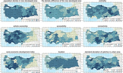
Table 3. Description statistics of observed values of the dependent and the explanatory variables.

	Dependent variable	POP_D	D_DIF	CENTR	V_OWN	ACCESS	CONCT	SOC_ECO	LOC	SD
Mean	−17.74	51.99	−28.85	1004.14	89.04	662.59	83.26	−.01	1.65	44.68
Median	−5.00	34.50	−26.34	668.11	101.01	282.00	48.00	.05	2.00	35.06
Std. Dev.	47.26	215.32	229.32	6103.88	42.73	1046.19	140.53	.33	.48	73.19
Variance	2233.75	46364.47	52588.19	37257374.81	1825.51	1094508.09	19749.19	.11	.23	5356.81
Range	314.00	2179.20	2154.29	47661.44	159.29	7109.00	880.00	1.51	1.00	558.75
Min.	−258.00	−468.60	−476.67	−26872.05	-.41	−50.00	−282.00	−.83	1.00	−259.13
Max.	56.00	1710.60	1677.62	20789.39	158.88	7059.00	598.00	.68	2.00	299.62
Sum	−1430.00	4211.10	−2336.73	81335.42	7212.05	53670.00	6744.00	−.08	134.00	3619.40

The analyses coloured using the Jenks natural breaks classification method are visualised in Figure 2. When the analysis of ‘population density in new developed area’ is examined, the western part of Türkiye has shown a largely homogeneous population density variation. The northern part and the eastern regions have the lowest and highest density changes. According to the analysis of ‘the density difference of the new developed area’, population densities in inhabited areas that were established from 1990 to 2018 show sprawl development or compact development. To put this into context, there are differences between the east and west of the country. While the eastern region is developing more widely, the western region has developed more compactly.

On centrality, a heterogeneous distribution is observed throughout the country. However, cluster regions are observed in the western part, in the central region and in the eastern part. In vehicle ownership, the highest vehicle ownership is seen in the south-west region and the north-central region, while the least ownership is largely in the south-east region. Accessibility values include the size of the urban area and the street connectivity effect. In this context, the spot areas with the lowest value are located in the eastern and central-northern regions of the country. Additionally, connectivity values show a heterogeneous distribution throughout the country. However, the socio-economic development index change based on the data of Dinçer et al. (2003) and The Ministry of Development (2013) has divided the country into three regions, namely the western, central and south-eastern regions. The regions where the decrease in index values is seen are the south-eastern region and the metropolitan cities of the country, Istanbul, Izmir, Ankara, Adana, and Gaziantep. The location variable classifies 28 coastal cities and the rest of cities as inland cities. The standard deviation of patches in urban areas shows the extent to which the built-up areas within the provincial boundaries differ. According to this variable, there is a distinctive difference in the southern and northern parts of the country. The northern part has smaller patches while the southern part has larger patches.

Estimation is an important part of spatial data science. ArcGIS and SPSS provide various estimation tools to support analyses. Therefore, the data of the study have been analysed using Forest-based Classification and Regression, Multiple Linear Regression, and Geographically Weighted Regression, which are developed by ArcGIS Pro software and IBM SPSS Statistics software.

2.3. Method

2.3.1. Random forest-based classification and regression (RFC)

The classification tree method (Dietterich 2000a, 2000b) is that they are boosting (Schapire et al. 1998) and bagging (Breiman 1996). A random forest was created by adding a layer of randomness to the bagging by Breiman (2001), which is compared to many other classifiers and is among the powerful algorithms available (Mitchell 1997; Genuer et al. 2010). The method is a bagged classification and regression tree (CART) method. It comes with various advantages such as the reduction in variance and the improvement of predictive accuracy of the methods, and disadvantages such as complex model structure and the importance of variable. Differences in variables to be predicted arise through the layouts of the trees (for the mathematical points, see by Breiman (1996, 2001), Smyth et al. (2015) and Grömping (2009)). Recently, the use of random forests has been considered in many scientific fields thanks to its contribution to the evaluation of variable effects (Breiman 2001; Rodriguez-Galiano et al. 2015; Georganos et al. 2021; Shang et al. 2021; Talebi et al. 2022). For example, these areas are remote sensing, geoscience, spatial cases, and estimating spatial data.

In the study, RFC method is used to create an estimation model with many variables. In the RFC model properties, the number of trees is 1000; the leaf size is 5; the tree depth range is 5-15; the mean tree depth is 9; the percentage of available per tree is 100; the number of randomly sampled variables is 3; the percentage of training data excluded for validation is 10. Model Out of Bag Errors are an indicator that will help validate the model. It also shows the performance gained by the number of trees in the model. The model dataset is randomly subdivided as 90% for the training set and 10% for the test set (Smyth et al. 2015).

2.3.2. Multiple linear regression (MLR)

Multiple linear regression is among the most common analysis tools used for estimation. The regression statistically measures and estimates the effects of explanatory variables on a dependent variable. Thus, MLR includes more than one explanatory variable. The equation of Multiple Linear Regression model is formulated (1) as in the following (Shen 2009; Olive 2017; Tranmer et al. 2020); (1) $$y_i={\beta }_0+{\beta }_1{x}_{i1}+{\beta }_2{x}_{i2}+\dots +{\beta }_n{x}_{in}+\mathrm{\varepsilon }\mathrm{ }$$(1) where x_i is the observed values; y_i is dependent variable; x_i is explanatory variables; βn represents slope coefficients of each explanatory variable; β₀ is y-intercept which is constant term; ɛ is the model’s error term, known as the residuals. The MLR is a non-spatial model.

2.3.3. Geographically weighted regression (GWR)

Geographically Weighted Regression (GWR) is one of the spatial methods and uses a linear regression (Fotheringham et al. 2002). The GWR model is the spatial relationships between the statistically significant variables. It generates statistical relationships between dependent and explanatory variables within the spatial bandwidth, which is one of the significant local parameters in the GWR model. It uses Variance Inflation Factor (VIF) to test collinearity among independent variables.

The GWR as a statistical model has a set of observations or locations {$x_{ij}$} for $i=1,\dots ,n$ cases and $j=1,\dots ,k$ explanatory variables, a set of dependent variables {$y_{ij}$}, and a set of location coordinates $\{(u_i,v_i)\}$ for each case. The equation of the Geographically Weighted Regression model is formulated (2) as in the following (Fotheringham et al. 2002; Brunsdon et al. 2010): (2) $$y_i={\beta }_0(u_i,v_i)+\sum _{j=1}^k{x_{ij}\mathrm{ }\beta }_j(u_i,v_i)+{\mathrm{↋}}_i\mathrm{ }$$(2) where β (coefficients) is computes by the regression tool, reflecting the relationship and the strength of each explanatory variable to the dependent variable; ↋ (residuals, residual errors) is the part of the dependent variable that is not explained by the method.

3. Results

This section provides the results of the RFC, the MLR, and the GWR models.

3.1. Random forest-based classification and regression (RFC) estimation model

In RFC method used with many variables, the percentage of variation explained indicates about 42% of the variability with 1000 trees in the population density. The variable of the density difference of the new developed area is of the highest importance at 33%, which means that it is the most useful in estimating the population density in the province. The importance of other variables is centrality at 16%, connectivity at 14%, population density in new developed area at 13%, number of vehicles per thousand people at 7%, socio-economic development index at 5%, location at 4%, accessibility at 4%, and the standard deviation of patches in urban area at 4%.

The value R² measures how well the model performs. The validation R² value is a better indicator of model performance than the training R². In the estimation model of this multivariate study estimating population density, the R² value in the training data (regression diagnosis) is 0.938 with an accuracy of approximately 94%. It is 0.802 with approximately 80% accuracy in the validation data (regression diagnostics). Explanatory Variables Range Diagnostics of training and validation using Forest-based Classification and Regression predict new population density. Values are reported based on 1000 trees within each forest (Table 4). The estimated explanatory variable range diagnostics lists the range of values covered by each explanatory variable in the datasets used to train and validate the model. For example, the number of vehicles per thousand people in the dataset used to train the model ranges from −0.41 to 158.88, and in the dataset used to validate the model, from 10.06 to 148.84% of the population density in the new developed area values used to train the model are used to validate the model. To minimise extrapolation, the validation values in Table 4 have been revised as density estimates.

Table 4. Range diagnostics of estimated explanatory variables.

	Training		Validation		Training share*	Validation share**
Variables	Minimum	Maximum	Minimum	Maximum
POP_D	−468.65	1710.61	−38.26	163.9	100	9
D_DIF	−476.67	1677.62	−219.62	77.67	100	14
CENTR	−11052.4	20789.39	−26872.1	10140.97	67	67
V_OWN	−0.41	158.88	10.06	148.84	100	87
ACCESS	−50.15	7058.66	148.44	3004.64	100	40
CONCT	−282	598	−111	338	100	51
SOC_ECO	−0.83	0.68	−0.45	0.66	100	74
LOC	1	2	1	2	100	100
SD	−259.13	198.63	−27.84	299.62	82	49

*Percent of overlap between the ranges of the training data and the input explanatory variable.

**Percent of overlap between the ranges of the validation data and the training data.

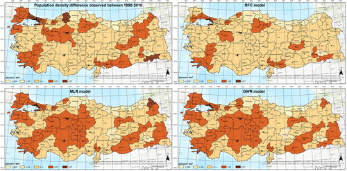
In terms of the estimated population density changes, the values of some provinces differ. A partial increase is observed in the estimated results of the observed density values. The estimated difference in population density is less than that observed in population density. However, while the urban area expands at the same rate and the population in the province increases at the same rate, the difference in population density is in the same range of values. Results show that for the population density difference excluding Istanbul, Bartın and Şırnak provinces, the estimated and observed values are almost equal in the provinces with values of 25 and below (Figure 3).

Figure 3. Population density difference observed between 1990-2018 (upper-left); estimated difference of population density in the RFC model (upper-right), the MLR model (bottom-left), and the GWR model (bottom-right) (people per square kilometre) (prepared by the author).

3.2. Multiple linear regression (MLR) estimation model

Table 5 shows that the most important explanatory variables in MLR model are centrality, vehicle ownership, and accessibility. The explanatory variables that are not statistically significant, indicated by a p-value greater than 0.05, are connectivity, socio-economic development index, location, and standard deviation of patches in urban area. However, VIF is used to test collinearity among the explanatory variables. The variables of population density in new developed area and the density difference of the new developed area have high values of VIF, which are 15.22 and 16.24, respectively. According to the results, since the VIF value is greater than about 10 (for redundancy among the explanatory variables), they are variables that are not fit for the MLR model. The results of the MLR model are visualised in Figure 3.

Table 5. Statistics of explanatory variables based on the MLR model.

Model	Unstandardized Coefficients		Standardized Coefficients	t	Sig.	Collinearity Statistics
	B	Std. Error	Beta			Tolerance	VIF
(Constant)	55.057	12.899		4.27	.000
POP_D*	−.66	.04	−2.98	−18.30	.000	.066	15.25
D_DIF	.66	.04	3.22	19.12	.000	.062	16.24
CENTR	.01	.00	.11	2.39	.020	.918	1.09
V_OWN	−.16	.07	−.14	−2.32	.023	.475	2.11
ACCESS	.01	.01	.16	3.26	.002	.698	1.43
CONCT	.01	.02	.01	.15	.879	.837	1.19
SOC_ECO	−.02	8.45	.00	−.01	.999	.497	2.01
LOC	−6.71	4.94	−.07	−1.36	.179	.698	1.43
SD	−.01	.03	−.02	−.37	.711	.917	1.09

*Dependent Variable: the difference in population density.

3.3. Geographically weighted regression (GWR) estimation model

GWR results are R² values 0.88 and R² adjusted values 0.86. The variables of population density in new developed area and the density difference of the new developed area indicate redundancy among explanatory variables, which are more than VIF value 7.5. Table 6 shows the results of the GWR model. The results are similar to the MLR model. The results of the GWR model are illustrated in Figure 3.

Table 6. Statistics of explanatory variables based on the GWR model.

Model	Coefficient	StdError	t-Statistic	Probability	Robust_SE	Robust_t	Robust_Pr	VIF
(Constant)	54.44	12.86	4.23	0.01*	11.31	4.81	0.01*
POP_D	−0.65	0.04	−18.32	0.00*	0.06	−10.96	0.00*	15.22
D_DIF	0.66	0.03	19.13	0.00*	0.06	11.25	0.00*	16.24
CENTR	0.00	0.00	2.40	0.02*	0.00	2.15	0.03*	1.09
V_OWN	−0.15	0.07	−2.29	0.02*	0.06	−2.59	0.01*	2.10
ACCESS	0.01	0.00	3.29	0.01*	0.00	3.45	0.01*	1.43
CONCT	0.00	0.02	0.13	0.89	0.01	0.15	0.88	1.19
SOC_ECO	−0.08	8.41	−0.01	0.99	6.64	−0.01	0.99	2.01
LOC	−6.53	4.93	−1.33	0.19	3.82	−1.71	0.09	1.43
SD	−0.01	0.03	−0.38	0.71	0.02	−0.43	0.67	1.09

*indicates a statistically significant p-value (p < 0.01)

4. Discussion

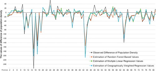
In this study, a comparative evaluation is made with the variables determined by referring to the importance of population density changes in terms of future spatial planning decisions through quantitative estimation methods. Figure 3 illustrates a spatial comparison of the results of all three models. The results of the study reveal that compared to the observed population density values, the estimation values of MLR and GWR models have higher values than the RFC model. Results of both models show regions where provinces with estimated density increases are clustered spatially (Figure 4).

Figure 4. Comparison of observed values and the performances of the RFC model, the MLR model, and the GWR model based on the difference in population density (people per square kilometre) (prepared by the author).

Current population density and the density in new developed area are influenced by the population density policy (Pendall 1999; Fulton et al. 2001). As population density increases, land consumption per person decreases (Pendall 1999; Ewing et al. 2003; Robinson et al. 2005; Yang et al. 2012; Faour 2015; Tikoudis et al. 2022). The results of this research support the idea that land consumption can be decreased if future ‘density allocation’ (Tikoudis et al. 2022) decisions are adapted to MLR results.

The important variables in the RFC model are seen as the density difference of the new developed area, centrality, and connectivity. Variables with significance relationships in MLR and GWR models are centrality, vehicle ownership, and accessibility. Ewing et al. (2003) states that the relationships between urban sprawl and transportation outcomes relate to density, land use mix, vehicle ownership, modes of transport, street accessibility, and centrality. This statement supports the results of this study. Although it is difficult to implement policies in the selection of vehicle ownership and modes of transport, the implementation of spatial policies on centrality, accessibility and population density allocation in new development areas may be among the possible decisions. The centrality variable is common to RFC, MLR, and GWR. The centrality identified in the study means that when the density increases, the distances between the settlements may decrease. The centrality variable is also supported by Pereira et al. (2013). Ewing et al. (2003) notes that vehicle ownership can be explained largely by population density; however, in the study, it is found that while vehicle ownership is significant in the MLR model, it is less important for the RFC model. The variables are seen as important for explaining population density.

Many urban density studies have been carried out in the planning literature, but limited resources have been found in the literature for estimating population density or urban density using new statistical tools and methods such as machine learning, deep learning, and spatial statistics (Wu et al. 2005; Georganos et al. 2021; Credit 2022), which can provide comparative forecast analyses with different methods. There is no one way to measure and estimate population density (Angel et al. 2020), thus the estimation methods used in this study are not the only way to measure.

In 2018, Türkiye’s population density was above the world average of 60 people per kilometre with a value of 107 people per kilometre (World Bank 2018). According to the results of this study, from 1990 to 2018, Türkiye’s average gross population density decreased by about 180 people per hectare, which means that a non-compact form of growth has been seen. This urban growth is one of the higher land consumption growth types (Pendall 1999; Robinson et al. 2005; Ng 2010; Faour 2015; Tikoudis et al. 2022). As Tikoudis et al. (2022) highlights, the strong correlation between density and urban growth provides a decisive role in the population density estimation comparisons and density allocations discussed in this research.

The density policy, therefore, refers to a more compact or a lower density development compared to the built-up area. For centrality, accessibility, and connectivity, the urban area is shaped by the road network (Bhatta et al. 2010); therefore, vehicle ownership, road density in urban area, and a significant increment in travel by vehicles, trigger spatial planning policies for urban expansion (Ewing et al. 2003; Pereira et al. 2013 ). Infrastructure investment or ownership is affected by socio-economic opportunities, which can change geographic locations (Yılmaz and Terzi 2021).

Population density is important spatial information for addressing the use and access to land resources in cities under the Sustainable Development Goals (Ehrlich et al. 2018). However, according to Tikoudis et al. (2022), urban population density estimation is among the important guides in making future ‘density allocation’ decisions on the macroscale.

5. Conclusions

This study examines RFC, MLR and GWR models and population density estimates both spatially and quantitatively, in which dependent and explanatory variables are included. Eighty-one city samples in Türkiye were examined to better understand how these models performed predictive values and whether the inclusion of spatial variables increased model performance. In the findings, it is observed that the confirmation rate increases as the number of trees increased for RFC, and for the MRL model different explanatory variables are needed. The two most important descriptive variables in the RFC model are the density difference of the new developed area and connectivity. On the other hand, the three main explanatory variables of MLR are centrality, vehicle ownership, and accessibility. While the RFC model is more consistent in density values in the new development areas, the importance of accessibility and connectivity is seen as more consistent in the MLR model.

Estimating population density and whether the urban area will be expanded or become more compact will guide the production of prevention strategies for future spatial planning policies. Thus, it can be used to estimate how much land will be consumed in the future. Therefore, in spatial planning policies, it is essential that decision-makers and policymakers obtain population estimates through various methods.

Ultimately, population density is a hierarchical and systematic structure. However, it is a useful tool to guide land use policy where the density value will be established from a holistic perspective. The introduction of new models to understand and predict density shows the importance of alternative methods. The models therefore support a new approach tool to explain the impact of population density on the planning process. Success in estimating population density will be possible by making population density measurement with more parameters.

Disclosure statement

The author declare that they have no conflicts of interest.

Data availability statement

The authors confirm that the data supporting the findings of this study are available within the article.

References

- Alexander D, Tomalty R. 2002. Smart growth and sustainable development: challenges, solutions and policy directions. Local Environ. 7(4):397–409.
- Al-Saaidy HJE, Alobaydi D. 2021. Studying street centrality and human density in different urban forms in Baghdad, Iraq. Ain Shams Eng J. 12(1):1111–1121.
- Anderson W, Guikema S, Zaitchik B, Pan W. 2014. Methods for estimating population density in data- limited areas: evaluating regression and tree-based models in Peru. PLOS. 9(7):1–15.
- Anderson WP, Kanaroglou PS, Miller EJ. 1996. Urban form, energy and the environment: a review of issues, evidence and policy. Urban Stud. 33(1):7–35.
- Angel S, Arango Franco S, Liu Y, Blei AM. 2020. The shape compactness of urban footprints. Prog Plann. 139:100429.
- Angel S, Lamson-Hall P, Blanco ZG. 2021. Anatomy of density: measurable factors that together constitute urban density. Buildings and Cities. 2(1):264–282.
- Bhatta B, Saraswati S, Bandyopadhyay D. 2010. Urban sprawl measurement from remote sensing data. Appl Geogr. 30(4):731–740.
- Boyko CT, Cooper R. 2011. Clarifying and re-conceptualising density. Prog Plann. 76(1):1–61.
- Breiman L. 1996. Bagging predictors. In: Quinlan R, editor, Machine learning. Vol. 24, Boston: kluwer Academic Publishers; p. 123–140.
- Breiman L. 2001. Random forests. In Schapire RE, editor. Machine learning. Vol. 45, The Netherlands: Kluwer Academic Publishers; p. 5–32.
- Brunsdon C, Fotheringham AS, Charlton ME. 2010. Geographically weighted regression: a method for exploring spatial nonstationarity. Geogr. Anal. 28(4):281–298.https://onlinelibrary.wiley.com/doi/10.1111/j.1538-4632.1996.tb00936.x
- Burchell RW, Downs A, McCann B, Mukherji S. 2005. Sprawl costs: economic impacts of unchecked development. Washington (DC): Island Press.
- Burton E, Jenks M, Williams K. 2003. The compact city: a sustainable urban form? London: Routledge.
- Camagni R, Gibelli MC, Rigamonti P. 2002. Urban mobility and urban form: the social and environmental costs of different patterns of urban expansion. Ecol Econ. 40(2):199–216.
- Churchman A. 1999. Disentangling the concept of density. J Plann Liter. 13(4):389–411.
- Cohen M, Gutman M. 2007. Density : an overview essay. Built Environ. 33(2):141–144.
- Credit K. 2022. Spatial models or random forest? Evaluating the use of spatially explicit machine learning methods to predict employment density around new transit stations in Los Angeles. Geog Anal. 54(1):58–83.
- Dietterich TG. 2000a. Ensemble methods in machine learning. In: Kittler J and Roli F, editors. Multiple classifier systems. Berlin: Springer; p. 1–15.
- Dietterich TG. 2000b. An experimental comparison of three methods for constructing ensembles of decision trees: bagging, boosting, and randomization. In: Fisher D, editor. Machine learning. Vol. 40. The Netherlands: Kluwer Academic Publishers; p. 139–157.
- Dinçer B, Özaslan M, Kavasoğlu T. 2003. İllerin sosyo-ekonomik gelişmişlik sıralaması araştırması. Ankara: T.C. Devlet Planlama Teşkilatı.
- Dovey K, Pafka E. 2014. The urban density assemblage: modelling multiple measures. Urban Des Int. 19(1):66–76.
- EEA. 2019. CORINE Land Cover. https://land.copernicus.eu/pan-european/corine-land-cover. [Accessed 18 December 2020].
- Ehrlich D, Kemper T, Pesaresi M, Corbane C. 2018. Built-up area and population density: two essential societal variables to address climate hazard impact. Environ Sci Policy. 90:73–82.
- Ewing R, Pendall R, Chen D. 2003. Measuring sprawl and its transportation impacts. Transp Res Rec. 1831(1):175–183.
- Ewing R. 1997. Is Los Angeles-style sprawl desirable? Am Plann Assoc. 63(1):107–126.
- Faour G. 2015. Evaluating urban expansion using remotely-sensed data in Lebanon. Leban. Sci. J. 16(1):23–32.
- Fotheringham AS, Brunsdon C, Charlton M. 2002. Geographically weighted regression: the analysis of spatially varying relationships. Hoboken, NJ: Wiley.
- Frenkel A, Ashkenazi M. 2008. Measuring urban sprawl: how can we deal with ıt? Environ Plann B Plann Des. 35(1):56–79.
- Fulton W, Pendall R, Nguyen M, Harrison A. 2001. Who sprawls most? how growth – patterns differ across the U.S. Washington, DC: Brookings Institution, Center on Urban and Metropolitan Policy; p. 1–23.
- Galster G, Hanson R, Ratcliffe MR, Wolman H, Coleman S, Freihage J. 2001. Wrestling sprawl to the ground: defining and measuring an elusive concept. Housing Policy Debate. 12(4):681–717.
- Genuer R, Poggi J-M, Tuleau-Malot C. 2010. Variable selection using random forests. Pattern Recog Lett. 31(14):2225–2236.
- Georganos S, Grippa T, Niang Gadiaga A, Linard C, Lennert M, Vanhuysse S, Mboga N, Wolff E, Kalogirou S. 2021. Geographical random forests: a spatial extension of the random forest algorithm to address spatial heterogeneity in remote sensing and population modelling. Geocarto International. 36(2):121–136.
- Gillham O. 2002. The limitless city : a primer on the urban sprawl debate. Washington (DC): Island Press.
- Grömping U. 2009. Variable importance assessment in regression: linear regression versus random forest. Am Stat. 63(4):308–319.
- Guastella G, Oueslati W, Pareglio S. 2019. Patterns of urban spatial expansion in European cities. Sustainability (Switzerland). 11(8):2247.
- Güneralp B, Zhou Y, Ürge-Vorsatz D, Gupta M, Yu S, Patel PL, Fragkias M, Li X, Seto KC. 2017. Global scenarios of urban density and its impacts on building energy use through 2050. Proc Natl Acad Sci U S A. 114(34):8945–8950.
- Hasse JE, Lathrop RG. 2003. Land resource impact indicators of urban sprawl. Appl Geogr. 23(2-3):159–175.
- Holden E, Norland IT. 2005. Three challenges for the compact city as a sustainable urban form: household consumption of energy and transport in eight residential areas in the Greater Oslo Region. Urban Stud. 42(12):2145–2166.
- Jongman B, Ward PJ, Aerts JCJH. 2012. Global exposure to river and coastal flooding: long term trends and changes. Global Environ Change. 22(4):823–835.
- KGM. 2019. Devlet ve İl Yolları Envanteri. Ankara: T.C. Ulaştırma ve Altyapı Bakanlığı. https://www.kgm.gov.tr/Sayfalar/KGM/SiteTr/Istatistikler/DevletveIlYolEnvanteri.aspx.
- Li L, Sato Y, Zhu H. 2003. Simulating spatial urban expansion based on a physical process. Landscape Urban Plann. 64(1–2):67–76.
- Lowry JH, Lowry MB. 2014. Comparing spatial metrics that quantify urban form. Comput Environ Urban Syst. 44:59–67.
- Magliocca N, McConnell V, Walls M, Safirova E. 2012. Explaining sprawl with an agent-based model of exurban land and housing markets. Resources for the Future. RFF DP 11:1–31.
- Malpezzi S. 2013. Population density: some facts and some predictions. Cityscape J of Policy Dev Res. 15(3):183–201.
- McFarlane C. 2016. The geographies of urban density: topology, politics and the city. Prog Human Geogr. 40(5):629–648.
- Mitchell TM. 1997. Machine learning. New York: McGraw-Hill.
- Ng E, editor. 2010. Designing high-density cities for social and environmental sustainability. London: Earthscan.
- OECD. 2012. Compact city policies: a comparative assessment. OECD Publishing.
- OECD. 2018. Rethinking Urban Sprawl: moving Towards Sustainable Cities. Paris: OECD Publishing.
- Olive DJ. 2017. Multiple linear regression. In: Linear regression. Cham: springer International Publishing; p. 17–83.
- OpenStreetMap 2017. www.openstreetmap.org.
- Owens SE. 1992. Land-use planning for energy efficiency. Appl Energy. 43(1-3):81–114.
- Pendall R. 1999. Do land-use controls cause sprawl? Environ Plann B. 26(4):555–571.
- Pereira RHM, Nadalin V, Monasterio L, Albuquerque PHM. 2013. Urban centrality: a simple index. Geogr Anal. 45(1):77–89.
- Rickwood P, Glazebrook G, Searle G. 2008. Urban structure and energy – a review. Urban Policy Res. 26(1):57–81.
- Robinson L, Newell JP, Marzluff JM. 2005. Twenty-five years of sprawl in the Seattle region: growth management responses and implications for conservation. Landscape Urban Plann. 71(1):51–72.
- Rodriguez DA, Targa F, Aytur SA. 2006. Transport implications of urban containment policies: a study of the largest twenty-five US metropolitan areas. Urban Studies. 43(10):1879–1897.
- Rodriguez-Galiano V, Sanchez-Castillo M, Chica-Olmo M, Chica-Rivas M. 2015. Machine learning predictive models for mineral prospectivity: an evaluation of neural networks, random forest, regression trees and support vector machines. Ore Geol Rev. 71:804–818.
- Salvati L. 2013. Urban containment in action? Long-term dynamics of self-contained urban growth in compact and dispersed regions of southern Europe. Land Use Policy. 35:213–225.
- Schapire RE, Freund Y, Bartlett P, Lee WS. 1998. Boosting the margin: a new explanation for the effectiveness of voting methods. Ann Statist. 26(5):1651–1686.
- Schneider A, Woodcock CE. 2008. Compact, dispersed, fragmented, extensive? A comparison of urban growth in twenty-five global cities using remotely sensed data, pattern metrics and census information. Urban Stud. 45(3):659–692.
- Schwarz N. 2010. Urban form revisited—selecting indicators for characterising European cities. Landscape Urban Plann. 96(1):29–47.
- Shang S, Du S, Du S, Zhu S. 2021. Estimating building-scale population using multi-source spatial data. Cities. 111:103002.
- Sharifi A. 2019. Resilient urban forms: a review of literature on streets and street networks. Build Environ. 147:171–187. Contents.
- Shen J. 2009. Linear regression.
- Silva M, Oliveira V, Leal V. 2017. Urban form and energy demand: a review of energy-relevant urban attributes. J Plann Liter. 32(4):346–365.
- Smyth D, Deverall E, Balm M, Nesdale A, Rosemergy I. 2015. Out-of-bag estimation. New Zealand Med J. 128(1425):97–100.
- Talebi H, Peeters LJM, Otto A, Tolosana-Delgado R. 2022. A truly spatial random forests algorithm for geoscience data analysis and modelling. Math Geosci. 54(1):1–22.
- The Ministry of Development. 2013. İllerin ve Bölgelerin Sosyo-Ekonomik Gelişmişlik Sıralaması Araştırması (SEGE-2011). Ankara: T.C. Kalkınma Bakanlığı.
- Tikoudis I, Farrow K, Mebiame RM, Oueslati W. 2022. Beyond average population density: measuring sprawl with density-allocation indicators. Land Use Policy. 112:105832.
- Tranmer M, Murphy J, Elliot M, Pampaka M. 2020. Multiple linear regression. 2nd ed. Manchester: Cathie Marsh Institute Working Paper.
- TURKSTAT. 2019. Turkish Statistical Institute. https://biruni.tuik.gov.tr/medas/?kn=95&locale=tr.
- Williams K, Burton E, Jenks M. 2000. Achieving sustainable urban form: an introduction. In Williams K, Burton E, Jenks M, editors. Achieving sustainable urban form. London: E & FN Spon.
- World Bank. 2018. Population density (people per sq. km of land area). https://databank.worldbank.org/source/world-development-indicators/Series/EN.POP.DNST.
- Wu S, Qiu X, Wang L. 2005. Population estimation methods in GIS and remote sensing: a review. GISci Remote Sens. 42(1):80–96.
- Yamagata Y, Seya H. 2013. Simulating a future smart city: an integrated land use-energy model. Appl Energy. 112:1466–1474.
- Yang J, Shen Q, Shen J, He C. 2012. Transport impacts of clustered development in Beijing: compact development versus overconcentration. Urban Stud. 49(6):1315–1331.
- Yılmaz M, Terzi F. 2021. Measuring the patterns of urban spatial growth of coastal cities in developing countries by geospatial metrics. Land Use Policy. 107:105487.