
 ?Mathematical formulae have been encoded as MathML and are displayed in this HTML version using MathJax in order to improve their display. Uncheck the box to turn MathJax off. This feature requires Javascript. Click on a formula to zoom.
Abstract
Airborne light detection and ranging (LiDAR) is a popular technology in remote sensing that can significantly improve the efficiency of digital elevation model (DEM) construction. However, it is challenging to identify the real terrain features in complex areas using LiDAR data. To solve this problem, this work proposes a multi-information fusion method based on PointNet++ to improve the accuracy of DEM construction. The RGB data and normalized coordinate information of the point cloud was added to increase the number of channels on the input side of the PointNet++ neural network, which can improve the accuracy of the classification during feature extraction. Low and high density point clouds obtained from the International Society for Photogrammetry and Remote Sensing (ISPRS) and the United States Geological Survey (USGS) were used to test this proposed method. The results suggest that the proposed method improves the Kappa coefficient by 8.81% compared to PointNet++. The type I error was reduced by 2.13%, the type II error was reduced by 8.29%, and the total error was reduced by 2.52% compared to the conventional algorithm. Therefore, it is possible to conclude that the proposed method can obtain DEMs with higher accuracy.
1. Introduction
The digital elevation model (DEM) plays an increasingly important role in disaster prevention and control, surveying and mapping resources and the environment, national defence, and other fields related to terrain analysis and the national economy. As LiDAR and airborne laser scanning (ALS) technologies continue to evolve, the acquisition of point cloud data has become increasingly fast and convenient. ALS can provide high precision and high density surface features and will also record point information regarding other surface (nonground) features, such as vegetation and buildings. The recorded information includes spatial coordinates, RGB colour, and reflection intensity (Yang et al. Citation2017). Considering that there is no obvious structural relationship between ground points and nonground points in ALS data, ALS point cloud filtering (Mongus and Žalik Citation2012; Wang and Zhang Citation2016) becomes difficult and troublesome during ALS data processing. However, the process of DEM production needs to distinguish ground points and nonground points in the point cloud data. ALS point cloud filtering comprises most of the ALS data processing workload, and the accuracy of DEM development is directly related to the results of ALS point cloud filtering.
Regardless of application, extracting DEM information from point clouds that contain ground points and nonground points is a fundamental step (Axelsson Citation1999; Wang et al. Citation2019). Conventional point cloud filtering methods can be classified into four categories according to their processing method, as follows:
Slope methods. This method maintains that the slope value of adjacent ground points is small, while the edges of nonground points can be identified by abrupt changes in slope values that continuously exceed the slope of the surrounding terrain (Vosselman Citation2000; Brzank and Heipke Citation2006). Therefore, the slope method can be implemented quickly without interpolation and retains the original topographic information well. However, the challenges with this method pertain to how to choose the appropriate threshold value for filtering different terrains.
Mathematical Morphology methods. The main principle of this method is that the nonground points undergo large changes to their elevation after morphological operations are applied, while ground points only undergo small elevation changes. The points with large elevation changes are judged as nonground points to be rejected by establishing an appropriate threshold (Zhang et al. Citation2003; Hui et al. Citation2016). There are two problems with this algorithm, however. The first problem involves the selection of the appropriate filter window. Second, this method makes it challenging to obtain good results over continuously undulating terrain. A morphological algorithm due to multilevel kriging interpolation was proposed by Hui et al. (Citation2016), which is an integration of a multilevel interpolation filtering algorithm and a progressive morphological filtering algorithm.
Surface methods. This method is based on the interpolation of ground surface points to build a rough surface model of the ground, and then the points that do not satisfy established conditions are gradually eliminated by setting certain filtering conditions (Chen et al. Citation2014). Continuous iterations are performed until the terrain accuracy requirements are satisfied (Kraus and Pfeifer Citation1998; Cai et al. Citation2019). A parameter-free multilayer progressive encryption filtering method was proposed (Mongus and Žalik Citation2014). This method first performs thin plate spline (TPS) interpolation at the topmost control point to obtain the topographic surface. Then, we calculate the distance from each control point in the lower layer to this surface and replace the control points with interpolated points if the distance is greater than an established threshold. This method performs gradual iterations until the distance to the bottom layer falls within the threshold, and filtering judgement are made for each point in the point cloud to obtain the result. Subsequently, Chen et al. (Citation2013) made improvements in the direction of seed point choices and filter judgements to improve the filtering accuracy. Hu et al. (Citation2014) also sampled TPS interpolation to achieve sufficient point cloud filtering, but while fitting the surface at each level, also calculated the curvature of the local area in each layer so that the filtering threshold could then be calculated automatically. The disadvantage is that the interpolation operation generally causes a loss of accuracy, the filtering results of each iteration are influenced by the results of the previous iteration, and the errors will be propagated and increased if the initial topographic surface is not accurate.
Progressive triangular irregular network methods. This method chooses the lowest point as the ground point and constructs a triangle from it, adding other points to the surface of the triangle within the limits of slope and distance. This algorithm can achieve a good effect in filtering; the disadvantage is that the process of creating the triangle network is complicated, consumes more memory, and takes a long time to filter. Additionally, this method is susceptible to negative outliers, which will draw the triangular surface downwards (Axelsson Citation2000; Wang et al. Citation2019). However, there are some newly proposed approaches, such as filtering based on expectation maximization and filtering using active learning strategies (Hui et al. Citation2019). Furthermore, deep learning methods have become more common and accessible as computer has improved and the increasing number of deep learning methods have been applied to point cloud data processing.
The PointNet neural network and its upgraded version, the PointNet++ neural network proposed by Qi et al. (Qi et al. Citation2017), can process 3D point clouds directly and achieve good results in point cloud classification (Yao et al. Citation2019; Briechle et al. Citation2020; Seo and Joo Citation2020; Chen et al. Citation2021). Klokov and Lempitsky (Citation2017) proposed a deep kd network that can take the colour, laser reflection intensity, and normal vector attributes of the data as input and structure the point cloud using the kd tree to learn and obtain the weights of each node in the tree. However, this network is sensitive to noise and rotation, and upsampling or subsampling operations are required for each point, which will additionally increase the computational complexity. Li et al. (Citation2018) proposed a simple and general point cloud feature learning framework, PointCNN, which uses a multilayer perceptron to learn and obtain a transformation matrix from the input to convert the disordered point cloud into an ordered one. However, the results of the transformation matrix are unexpected, and the ordering problem of point clouds is still difficult. Moreover, as this method is intended for classifying a single point cloud model, the classification of point clouds for complex scenes remains a problem that needs to be resolved. Wen et al. (Wen et al. Citation2020, Citation2021) proposed a neural network named D-FCN with directional constraints and a global-local graph attention convolution neural network (GACNN), which can take the intensity and raw three dimensional coordinates as input. Therefore, it can be directly applied to the semantic labelling of unstructured three dimensional point clouds. Li et al. (Citation2020) proposed a geometry-attentional network that consisted of geometric perceptron convolution, dense hierarchies, and elevation attention modules. These three features can be effectively embedded and trained in an end-to-end manner. Jin et al. (2021) proposed a point based fully convolutional neural network that extracted point features and block features to classify each point by its geometric information. Hu et al. (Citation2020) proposed a RandLA-Net that can directly infer the semantics of each point for large-scale point clouds with efficient and lightweight features.
Existing traditional methods have achieved good results in point cloud filtering. However, they still require complex parameter tuning when encountering various types of urban, mountains, and forested terrain. Parameter tuning is usually time consuming, and generating DEMs from filtered point cloud data incurs large manual editing costs. As a result, these algorithms are not easy to reproduce for inexperienced users. To solve this problem, this study proposes a deep learning algorithm based on a multi-information fusion PointNet++ neural network. The proposed algorithm is developed based on the semantic segmentation of point clouds. The improved PointNet++ neural network separates ground and nonground points from the point cloud and performs point cloud segmentation. The low density datasets provided by the International Society for Photogrammetry and Remote Sensing (ISPRS) and the high density datasets provided by the United States Geological Survey (USGS) were used to test the algorithm proposed in this article. Experimental results show that the proposed multi-information fusion PointNet++ method achieves good performance under a variety of terrain features with less human manipulation. Thus, the proposed method will be user friendly and thereby provide a good foundation for DEM development from airborne LiDAR.
2. Methodology
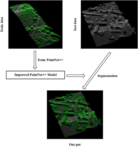
Airborne point cloud filtering means distinguishing ground points from nonground points in airborne point cloud data. Therefore, the point cloud filtering method can be treated as a binary classification problem. The experimental data were divided into ground points and nonground points and labelled accordingly. Eighty percent of the data were randomly selected as the training set, and the rest were selected as the test set. The deep learning model is trained from the training set and used to predict and classify the test set. The overall data processing flowchart of the ground segmentation method is shown in ().
Figure 1. Flowchart of the proposed approach.
2.1. PointNet++ neural network
PointNet is a neural network that can directly process point cloud data, and its segmentation method is shown in (). By using the symmetric max pooling function, the problem of unordered point sets can be effectively solved. The T-net convolutional network is used to generate the affine transformation matrix, which makes the translation and rotation operations of the point set more robust. The core layer of this network is max pooling, where the global features of the overall point cloud are extracted, and segmentation is achieved by stitching the local features with the global features and then classifying each point by a multilayer perceptron. Then, new features are extracted according to the combined point features. Finally, each point of the new features is attributed based on the local and global information.
Figure 2. PointNet segmentation network.
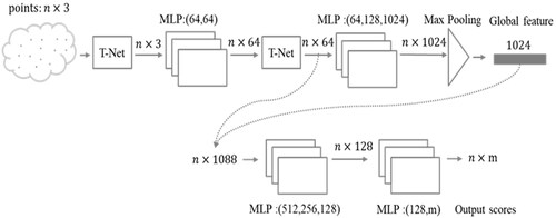
EquationEquation (1)(1)
(1) is expressed as a set of points mapped to a vector, as follows:
(1)
(1)
In the formula, is the point cloud data,
is the continuous set function,
represents max pooling, and
represents the multilayer perceptron (MLP) network.
The PointNet network poorly captures the local features in the study space since it focuses on the global features. Therefore, the PointNet++ network was proposed to process a set of points hierarchically sampled in a metric space. PointNet++ borrows the idea of a convolutional neural network (CNN), which is a multilayer perceptual field network, and designs a set of relationships to extract features from the point cloud so that layer features can eventually be extracted. As seen from (), the PointNet++ neural network structure is a combination of two abstraction modules (set abstraction, SA), which then uses PointNet to extract features. Finally, the point cloud is restored to the original quantity using the interpolation method and obtains scores for each point.
Figure 3. PointNet++ segmentation network.
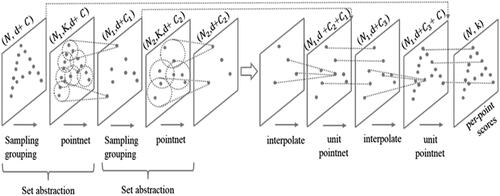
The core of the PointNet++ neural network is the SA level. Each SA level is divided into the sampling layer, the grouping layer, and the PointNet layer. The SA module takes an matrix as input. N refers to the number of points,
is the coordinate of the point dimension and
is the feature dimension of the point. It outputs an
matrix of
subsampled points.
The SA level plays a subsampling role. Iterative farthest point sampling (FPS) is used to choose a set of points in the sampling layer. The input of the grouping layer is the matrix and the coordinates of a set of centroids of size
is the number of points about centroid points. For example, in the grouping layer, if
neighbourhood points are selected in the local area of each sampling point and the aggregate input is
then the output is a group of point sets of size
Finally, the local feature results in the sampling area are extracted through PointNet, converted into the size of
and used as the input of the next SA layer. Point cloud segmentation needs to obtain the features of each point, and it needs to go through multiple upsampling operations until the original number of point clouds is restored. A full connection operation is performed on each point to obtain all classifications.
2.2. RGB and normalized coordinate information
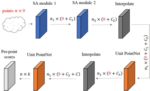
Airborne point cloud data usually contain coordinates, RGB data, and intensity information. However, both PointNet and PointNet++ neural networks only use the three dimensional coordinates of the point cloud as the input information. The information from the point cloud is not fully utilized. Therefore, apart from using the 3D coordinate information of the point cloud data, we also artificially add RGB data as well as the normalized coordinate information to each point. We render colours according to the category of each point. Each point has a corresponding label in the point cloud data, we perform a batch operation on the point cloud data by writing a Python script that assigns different colours to the labels identified. This enables the artificially add RGB information data. Then, the input channels are expanded by adding the RGB information and the normalized coordinate instead of only using geometric information to perform convolution operations.
The input of the raw SA level is where
represents the points number, and
represents the dimension (PointNet++ uses XYZ coordinates, then
is equal to 3). After adding RGB and normalized coordinate information, the input matrix is
Coordinate normalization converts the coordinates of all points into a unified coordinate system relative to the centre of mass, as follows:
(2)
(2)
(3)
(3)
(4)
(4)
In the formula,
and
is the centre of mass coordinate. Normalized coordinate information helps to capture the relationship between points in a local area. On the other hand, RGB describes the surface properties of different classes of objects. The surface properties of the same classes of objects are approximately the same, but the RGB data is not sensitive to changes in size and direction. Therefore, the RGB values are combined with the original coordinates and normalized coordinates can adequately capture the local features during feature extraction.
In this way, the convolutional networks can perform feature extraction not only by extracting the 3D coordinate information from the point cloud, but also by learning the RGB and the normalized coordinate information. Changing from the original matrix to the
matrix for increased multidimensional convolution can extract deeper features between the point relationships, which can partially improve the accuracy of the algorithm. The multi-information fusion PointNet++ is shown in ().
Figure 4. Improved PointNet++ segmentation network.
2.3. Experimental data
The low density data provided by the International Society for Photogrammetry and Remote Sensing (ISPRS) and the high density data provided by the United States Geological Survey (USGS) are used to validate the algorithm proposed by this study. As the raw experimental data do not contain RGB information, we render the point cloud colours based on their category. We choose Samp11 of the ISPRS data for demonstration, as shown in ().
Figure 5. ISPRS data without RGB information (left), ISPRS data with RGB information rendered by category (right). Red points: roofs of buildings, green points: ground points, blue points: nonground points.
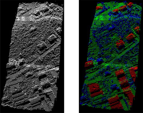
The ISPRS dataset can be accessed by the website http://www.itc.nl/isprswgIII-3/filtertest/. The average point spacing of the ISPRS dataset is 1–3.5 m, which is much lower than the point cloud density of approximately 15 points/m2 collected by the current equipment, so only the filtering performance of the low density point cloud dataset can be verified. An Optech ALTM scanner was used to collect the ISPRS dataset, which consisted of eight sites with different environments (sites 1–8). These samples were corrected by semiautomatic filtering and visual discrimination, and all points were accurately classified into ground points and nonground points. The dataset includes steeply sloping terrain, dense vegetation, buildings with vegetation, train stations, multistory buildings with courtyards, quarries (with fracture lines), and data gaps. To assess the precision of the method proposed in this article, we selected fifteen reference samples from sites 1–7 with different topographic features and land cover types. Because of the lack of reference data, site 8 was excluded. The urban point density is 0.4–1 point/m2 with a point spacing of 1–3.5 m, and the rural point density is 0.08–0.25 point/m2 with a point spacing of 2–3.5 m.
The USGS dataset can be accessed by the website: https://apps.nationalmap.gov/lidar-explorer/. The USGS dataset with a point spacing of approximately 0.5 m and an average point density of approximately 3–4 points/m2 is additionally selected to validate the filtering performance. The USGS benchmark dataset can verify the filtering performance of the high density point cloud dataset. The USGS dataset was collected by a linear mode LiDAR sensor, and all points were accurately labelled and classified as ground points and nonground points. Similarly, we manually rendered the point cloud colours based on their category. The selected region is the South St. Louis region of the United States. Forest areas were mainly selected, and the dataset included steep terrain, dense vegetation, and fractured terrain with mixed vegetation. The area of the selected region is approximately 47 square kilometres. We selected three reference samples from which to verify the accuracy of the method proposed in this work. It is also possible to verify how well deep learning methods perform in extracting DEMs in forested areas. All the samples and associated features are listed in ().
Table 1. Characteristics of sample.
2.4. Accuracy evaluation index
In this study, three accuracy metrics are used to analyze the accuracy of our proposed method, including type I error (ground points misclassified as nonground points), type II errors (nonground points misclassified as ground points), and the total error (the proportion of type I and II error points to total points). Type I error reflects the performance of the method in retaining ground points. Type II error reflects the performance of the method in removing nonground points, and the total error reflects the balance and practicality of the method.
Additionally, the Kappa coefficient is calculated. This coefficient can compare the consistency of reference data and experimental data, which is a more robust measure. The specific calculation formulas for each index can be found in () and (EquationEquations (5)–(8)).where a is the number of correctly classified ground points, b is the number of ground points incorrectly classified as nonground points, c is the number of nonground points misidentified as ground points, and d is the number of correctly classified nonground points.
Table 2. Calculation equations of error and Kappa coefficient.
3. Experimental results and analysis
3.1. Experimental results
To qualitatively evaluate the performance of the algorithm under different terrain conditions. All 15 samples provided from ISPRS are predicted in this work. Seven of the results are selected for presentation, as shown in ().
Figure 6. Results of each group. Columns (a): DSMs, (b): DEMs produced from the references, (c): DEMs produced by our method, (d): Type I and type II error spatial distributions.
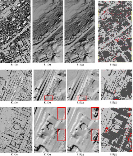
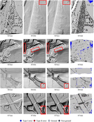
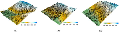
Figure 7. Digital surface models of the three samples.
The inverse distance weighting method is used to generate DEMs with a 1 m × 1 m resolution to analyze the accuracy of the method proposed here. The red rectangular regions indicate the difference between the predicted DEM and the original DEM.
The terrain of S11 in () is a hillside, and the nonground point objects contain vegetation and buildings that are mostly rectangular. From the comparison between the DEM S11(c) in obtained by the method presented in this paper and the DEM S11(a) in obtained by the reference data, we see that our proposed method can adequately filter out the buildings and the vegetation around the buildings. The agreement is good with the reference DEM in S11(b) in . The nonground point objects of S22 mainly contain irregularly shaped buildings, bridges, and other targets. The comparison between DEM image S22 (c) and the reference DEM image S11 (b) shows that our algorithm eliminates the bridge portion of S22, but there is some type II errors in the lower boundary of the image. The area of S23 mainly contains large irregular buildings. Type II errors occur on the image boundaries because the level surfaces of large buildings are similar to the planar surface features. The data in S51 are mainly vegetation on steep slopes. The comparison between DEM image S51(c) and the reference DEM image S51(b) shows that all vegetation on the slope is accurately filtered out by our method. However, there are some type I errors at the upper right boundary of the image that can be removed by subsequent manual editing. The area of S53 is mainly intermittent terrain, and the vegetation is distributed on the slope of the terraces. The results in S53(c) show that the buildings on the fault can be sufficiently filtered. However, there is a misclassification at the boundary resulting in type I errors. The data in S61 are characterized by discontinuous terrain and missing data. The error classification of S61(d) shows that type I errors mostly occur at the boundaries of the image. The area of S71 contains underground passages, bridges, etc. The comparison between the DEM image S71(c) obtained by this algorithm and the DEM image S71(b) obtained by the reference data shows that the bridges are accurately filtered out and the ground points can be correctly categorized and retained. The above analysis shows that our algorithm offers a good filtering effect for different types of areas.
shows that the type I errors occurred at an average rate of 1.24% for the 15 samples, and the type I error of the S42 and S54 samples is zero. All the ground points were classified correctly, and the Kappa coefficients also reach 94.46% and 99.02%, respectively. The average rate that type II error occurred was 1.91% from all samples. Among them, the type II errors of S51, S53, and S61 are zero, indicating that the nonground points are all classified correctly. This indicates that the method we proposed has a highly accurate filtering effect for both ground and nonground points. The average total error of all samples can reach 1.93%, and the lowest total error is only 0.43% in S12. The highest kappa coefficient is 99.12% in S12. The average kappa coefficient of all samples is 91.80%.
Table 3. Error and Kappa coefficient of the ISPRS & USGS test set.
From () and the comparison between the errors from of this new method and the traditional method in (), it can be seen that the method we propose has better filtering accuracy for both flat and steep terrain, which shows that the deep learning method has good applicability and reliability. The difference is that the traditional algorithm needs to set different parameters for different terrains to achieve sufficient filtering accuracy.
Table 4. Comparison of traditional filtering algorithms applied to the ISPRS dataset.
The reference DEM generated using the original ground points from the USGS data is shown in ( (b1) (c1)), and the predicted DEM produced from the ground points extracted by our proposed method is shown in ( (b2) (c2)). From the comparison between the reference DEM and the prediction DEM, it is obvious that the DEM obtained by the deep learning method shown in scene (a) is smooth, and the terrain details are preserved more completely without producing a surface that is too rough or that has excessive distortion. Scene (b) has good detail retention in the terrain breaks, but some terrain details are lost in the local area. The predicted DEM of Scene (c) is very similar to the reference DEM.
Figure 8. Reference data and interpolated DEMs of the proposed method.
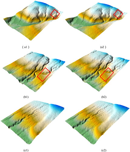
The ISPRS dataset, which had a low point cloud density, and the USGS dataset, which had a higher point cloud density, were used to verify the reliability of the method. This showed that the proposed method can be used for accurate point cloud filtering and DEM generation.
3.2. Quantitative analysis
shows each error index and Kappa coefficients, determined by the method presented in this paper, for 15 measurement areas. In addition, our method is compared with the original PointNet++ neural network as well as the algorithms proposed and tested by ISPRS scholars in recent years. The applicability and reliability of this new method are demonstrated by comparing it with traditional algorithms. Type I errors refer to the percentage of misclassified ground points, type II errors refer to the percentage of misclassified nonground points, and the total error is the total probability of points being misclassified. The specific data are shown in ( and ).
Figure 9. Comparison with other methods and our method using 15 samples from the ISPRS dataset. Error rates of PointNet++; error rates of Mongus (2012); error rates of Mongus (2014); error rates of Hu (Citation2014) error rates of Chen (Citation2013); error rates of Zhang et al. (Citation2016); error rates of Hui (Citation2016); error rates of Ours.
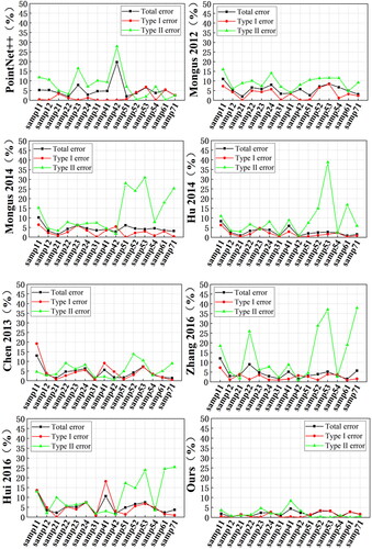
Table 5. Comparison of deep learning models applied the ISPRS dataset.
and show the results of comparing the method from this study with the original PointNet++ neural network and six other traditional filtering methods. From the table, the average value of the type I error for the six traditional filtering algorithms is 3.37%, and the minimum value is 1.84% for the method used by Hu et al. (Citation2014). The average value of the type II error is 10.2%, and the minimum value is 5.63% for the method proposed by Chen et al. (Citation2013). The average value of the total error is 4.45%, and the minimum value is 2.86% for Hu et al. (Citation2014).
The method used in this study produced a type I error of 1.24%, a type II error of 1.91%, and a total error of 1.93%. The type I error of the original PointNet++ neural network is 1.75%, the type II error is 8.06%, and the total error is 5.34%. Compared to the original PointNet++ neural network, the proposed method reduces the type I error, type II error, and total error by 0.51%, 6.15%, and 3.41%, respectively. Compared with the six traditional algorithms, the type I error, type II error, and total error are reduced by an average of 2.13%, 8.29%, and 2.52%, respectively. The method presented in this paper can generate high quality DEMs, especially those retaining subtle, minute, and steep terrain. Traditional algorithms may produce more type I errors. This result suggests that DEM production requires only simple manual postediting because it is usually easier to eliminate nonground points (type II errors) than to find erroneous ground points.
shows the results of data filtering according to the method we proposed, the method of the original PointNet++ neural network, and the other 6 traditional filters for 15 survey areas. The topography of measurement areas S12, S21, and S31 is relatively gentle, and the change in slope is small. Therefore, the filtering effect is more satisfactory. The total error for area S12 is 0.43% in this study, which is the lowest error among all filtering algorithms. With the gradual increase in slope, the error increases, and the total errors of S52 and S53 are 3.23% and 3.20%, respectively, which are much higher than that of the more gently sloped areas, but it is also the best among all the methods. This is probably due to the difficulty of capturing point feature information in places with large topographic relief and due to the influence of variable point cloud densities. From the line graph, we can see that our proposed method maintains good filtering accuracy for all kinds of terrain, and the lines are smoother than the other methods, which produce large fluctuations. However, no one filtering algorithm can obtain the best results across all terrains, and users need to choose the right method and set the relevant parameters according to the terrain. However, the deep learning method can obtain relatively reliable filtering results for different terrains without setting too many parameters.
4. Discussion
This method can be applied to point cloud data obtained from airborne LiDAR systems, and there is no restriction on the type, flight altitude, and PRF. The traditional point cloud filtering algorithm offers the benefits of simple principles and easy implementation. However, this type of algorithm is not without problems. Specifically, the algorithm used by the traditional methods is dependent on the threshold setting. If the threshold setting is not correct, it is difficult to obtain the ideal filtering results. Different algorithms, parameters, and thresholds are needed for different terrains to obtain the ideal filtering results. These traditional methods can achieve good point cloud filtering results but generating DEMs based on filtered point cloud data still requires considerable labour.
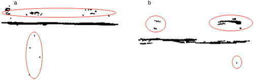
However, deep learning methods do not need to set as many parameters and thresholds when compared to traditional methods. Instead, a large amount of labelled data is needed for model training, and the filtering accuracy can be improved by adding samples with different terrain features. However, there are some cases that our method cannot handle well. As shown in (), this method produces some erroneous type II error classification results. These erroneous nonground points belong to very low or very high anomalies or the flat roofs of buildings. These errors arise mainly due to classifying point clouds with similar characteristics that do not belong to the same class as belonging to the same class during the feature extraction step. In samp31 and samp41, there are very low anomalies that are not removed and the roofs of buildings are misclassified as ground points. Such problems can be eliminated by the visual discrimination method, which is also an area that must be improved.
Figure 10. (a) The deep learning model accepts incorrect ground points in samp31. (b) The deep learning model accepts incorrect ground points in samp41.
5. Conclusion
In this study, a multi-information fusion PointNet++ neural network model was proposed to apply deep learning methodologies to point cloud filtering. This method offers improvements on the input side of the neural network. Using the point cloud 3 D coordinate information, additional RGB data and normalized coordinate information are added to enrich the input information dimension. Tests were conducted using the ISPRS benchmark dataset and USGS benchmark dataset with different terrains and different point cloud densities. Compared with the other traditional algorithms, the type I error, type II error, and total error were reduced by an average of 2.13%, 8.29%, and 2.52%, respectively. Compared with the original PointNet++ neural network, the type I error, type II error, and total error were reduced by 0.51%, 6.15%, and 3.14%, respectively. The results showed that the method presented in this paper has higher accuracy and outperforms the traditional algorithms. In the results of 15 samples selected from the ISPRS dataset, the type I error was 1.24%, the type II error was 1.91%, the total error was as high as 1.93%, and the kappa coefficient reached 91.80%. Once the type I and II errors had been sufficiently reduced by this method, better point cloud filtering accuracy and DEM construction accuracy could be obtained. This method offers wide applicability and good reliability, and it performs well over a variety of terrains, unlike the traditional method of filtering data over certain terrains.
Acknowledgements
We would also like to thank the data providers of the ISPRS and USGS. Supplementary data associated with this article can be found in the online version at http://www.itc.nl/isprswgIII-3/filtertest/and https://apps.nationalmap.gov/lidar-explorer/.
Disclosure statement
No potential conflict of interest was reported by the authors.
Correction Statement
This article has been corrected with minor changes. These changes do not impact the academic content of the article.
Additional information
Funding
7. References
- Axelsson P. 1999. Processing of laser scanner data—algorithms and applications. ISPRS J Photogramm Remote Sens. 54(2-3):138–147.
- Axelsson P. 2000. DEM generation from laser scanner data using adaptive TIN models. Int Arch Photogramm Remote Sens. 33(4):110–117.
- Briechle S, Krzystek P, Vosselman G. 2020. Classification of tree species and standing dead trees by fusing UAV-based lidar data and multispectral imagery in the 3D deep neural network PointNet++. ISPRS Ann Photogramm Remote Sens Spatial Inf Sci. V-2-2020:203–210.
- Brzank A, Heipke C. 2006. Classification of Lidar data into water and land points in coastal areas. Remote Sens Spatial Inform Sci. 36:197–202.
- Cai S, Zhang W, Liang X, Wan P, Qi J, Yu S, Yan G, Shao J. 2019. Filtering airborne LiDAR data through complementary cloth simulation and progressive TIN densification filters. Remote Sens. 11(9):1037.
- Chen C, Li Y, Li W, Dai H. 2013. A multiresolution hierarchical classification algorithm for filtering airborne LiDAR data. ISPRS J Photogramm Remote Sens. 82:1–9.
- Chen Y, Liu G, Xu Y, Pan P, Xing Y. 2021. PointNet++ network architecture with individual point level and global features on centroid for ALS point cloud classification. Remote Sens. 13(3):472.
- Chen YF, Hou YF, Xu Q, Xing S, Li J. 2014. LiDAR points cloud filtering method based on adaptive morphological. J Geomat Sci Technol. 31(6):603–607.
- Hui Z, Jin S, Cheng P, Ziggah YY, Wang L, Wang Y, Hu H, Hu Y. 2019. An active learning method for DEM extraction from airborne LiDAR point clouds. IEEE Access. 7:89366–89378.
- Hui Z, Li D, Jin S, Ziggah YY, Wang L, Hu Y. 2019. Automatic DTM extraction from airborne LiDAR based on expectation-maximization. Opt Laser Technol. 112:43–55.
- Hui Z, Hu Y, Yevenyo YZ, Yu X. 2016. An improved morphological algorithm for filtering airborne LiDAR point cloud based on multi-level kriging interpolation. Remote Sens. 8(1):35.
- Hu H, Ding Y, Zhu Q, Wu B, Lin H, Du Z, Zhang YT, Zhang YS. 2014. An adaptive surface filter for airborne laser scanning point clouds by means of regularization and bending energy. ISPRS J Photogramm Remote Sens. 92:98–111.
- Hu Q, Yang B, Xie L, Rosa S, Guo Y, Wang Z, Trigoni N, Markham A. 2020. Randla-net: efficient semantic segmentation of large-scale point clouds. In Proceedings of the IEEE/CVF Conference on Computer Vision and Pattern Recognition. p. 11108–11117.
- Huang R, Xu Y, Stilla U. 2021. GraNet: global relation-aware attentional network for semantic segmentation of ALS point clouds. ISPRS J Photogramm Remote Sens. 177:1–20.
- Kraus K, Pfeifer N. 1998. Determination of terrain models in wooded areas with airborne laser scanner data. ISPRS J Photogramm Remote Sens. 53(4):193–203.
- Klokov R, Lempitsky V. 2017. Escape from cells: deep kd-networks for the recognition of 3d point cloud models. In Proceedings of the IEEE International Conference on Computer Vision. p. 863–872.
- Li Y, Bu R, Sun M, Wu W, Di X, Chen B. 2018. PointCNN: convolution on X-Transformed points. In: Advances in Neural Information Processing Systems; p. 828–38.
- Li W, Wang FD, Xia GS. 2020. A geometry-attentional network for ALS point cloud classification. ISPRS J Photogramm Remote Sens. 164:26–40.
- Mongus D, Žalik B. 2012. Parameter-free ground filtering of LiDAR data for automatic DTM generation. ISPRS J Photogramm Remote Sens. 67:1–12.
- Mongus D, Žalik B. 2014. Computationally efficient method for the generation of a digital terrain model from airborne LiDAR data using connected operators. IEEE J Sel Top Appl Earth Observ Remote Sens. 7(1):340–351.
- Qi CR, Su H, Mo K, Guibas LJ. 2017. Pointnet: deep learning on point sets for 3d classification and segmentation. In Proceedings of the IEEE conference on computer vision and pattern recognition. p. 652–660.
- Qi CR, Su H, Mo K, Guibas LJ. 2017. Pointnet++: deep hierarchical feature learning on point sets in a metric space. Adv Neur Inform Process Syst. 30
- Seo H, Joo S. 2020. Influence of preprocessing and augmentation on 3D Point cloud classification based on a deep neural network: PointNet. In 2020 20th International Conference on Control, Automation and Systems (ICCAS). pp. 895–899
- Vosselman G. 2000. Slope based filtering of laser altimetry data. Int Arch Photogramm Remote Sens. 33(B3/2; PART 3):935–942.
- Wang L, Zhang Y. 2016. LiDAR ground filtering algorithm for urban areas using scan line based segmentation. arXiv preprint arXiv:1603.00912
- Wang J, Zhang X, Hong S, Chen Y. 2019. Aerial LiDAR point cloud filtering algorithm combining mathematical morphology and TIN. Sci Survey Mapp. 44(05):151–156.
- Wen C, Li X, Yao X, Peng L, Chi T. 2021. Airborne LiDAR point cloud classification with global-local graph attention convolution neural network. ISPRS J Photogramm Remote Sens. 173:181–194.
- Wen C, Yang L, Li X, Peng L, Chi T. 2020. Directionally constrained fully convolutional neural network for airborne LiDAR point cloud classification. ISPRS J Photogramm Remote Sens. 162:50–62.
- Yao X, Guo J, Hu J, Cao Q. 2019. Using deep learning in semantic classification for point cloud data. IEEE Access. 7:37121–37130.
- Yang B, Liang F, Huang R. 2017. Progress, challenges and perspectives of 3D LiDAR point cloud processing. Acta Geodaet Cartograph Sin. 46(10):1509–1516.
- Zhang K, Chen SC, Whitman D, Shyu ML, Yan J, Zhang C. 2003. A progressive morphological filter for removing nonground measurements from airborne LIDAR data. IEEE Trans Geosci Remote Sens. 41(4):872–882.
- Zhang W, Qi J, Wan P, Wang H, Xie D, Wang X, Yan G. 2016. An easy-to-use airborne LiDAR data filtering method based on cloth simulation. Remote Sens. 8(6):501.