Estimating forest aboveground biomass using temporal features extracted from multiple satellite data products and ensemble machine learning algorithm

Abstract

Many studies have attempted to estimate forest aboveground biomass (AGB) from satellite data accurately. Temporal information may be beneficial to AGB estimation but remains underexplored. Thus, this paper aims to investigate whether and how temporal features extracted from multiple satellite-derived data products can improve prediction accuracy. To this end, we develop four methods to exploit the temporal features of moderate resolution imaging spectroradiometer (MODIS) data products: the method that uses all annual features (AAF), the method that selects essential features based on the Spearman correlation coefficient (SCC) criterion, the method that employs the seasonal average and principal component analysis (PCA) components (SAP), and the method that includes phenological characteristic parameters (PCP) as the predictors of forest AGB. Lidar-derived forest AGB in California serves as the reference AGB data, and the XGBoost ensemble algorithm is utilized to model forest AGB with temporal features of MODIS data products. The results demonstrate that the AAF-based features lead to the most accurate AGB prediction, whereas using information extracted by SAP and PCP gives rise to less accurate results. Annual MODIS surface reflectance data combined with forest canopy height can provide the AGB estimates, with an average R-squared (R²) of 0.58 and root-mean-squared error (RMSE) of 147.58 Mg/ha. The results of this study highlight the necessity of utilizing annual time-series data, particularly the annual surface reflectance data, for AGB prediction.

Keywords:

• Time-series data
• forest aboveground biomass
• phenology
• MODIS data
• XGBoost

1. Introduction

Forest aboveground biomass (AGB) plays a vital role in the global carbon cycle and climate change mitigation and has been identified as an essential climate variable by the Global Climate Observing System (GCOS) (Le Toan et al. 2011; Dhillon and Von Wuehlisch 2013; Mitchard 2018). Many recent studies have focused on forest AGB estimation and mapping by combining optical imagery, synthetic aperture radar (SAR), and lidar (Amini and Sumantyo 2009; Song 2012; Ahmed et al. 2013; Sinha et al. 2015; Moradi et al. 2022; Nuthammachot et al. 2022). Some forest AGB maps have thus been generated on regional or global scales (Saatchi et al. 2011; Baccini et al. 2012; Zhang et al. 2019). However, evaluation and comparison results indicate significant uncertainties in these biomass maps. Various studies have provided different data on the magnitude and spatial distribution of forest AGB prediction (Mitchard et al. 2013; Zhang et al. 2019), hindering its further application and indicating the vital necessity for improving AGB estimation.

Some studies have extracted spatial information (e.g. texture metrics) from remote sensing images as predictors of forest AGB to improve prediction accuracy (Sarker et al. 2013; Li et al. 2020). However, the primary data sets have been acquired within specific time, and the saturation problem at lower AGB values and poor accuracy of AGB estimates leave much room to improve (Zhu and Liu 2015). Other studies have suggested that time-series data can provide more information on AGB prediction than single-temporal data and have enhanced the accuracy of forest AGB estimation (Le Maire et al. 2011; Kamir et al. 2020; Nguyen et al. 2020). For example, Zhu and Liu (2015) found that the Landsat normalized difference vegetation index (NDVI) in fall (e.g. September 24) had a stronger relationship with forest AGB than the commonly used peak season NDVI (e.g. June 20), with a correlation coefficient of 0.638 compared to 0.457. They also reported that using NDVI based on seasonal time series resulted in an accurate estimation of forest AGB. Zhang et al. (2014b) compared the performance of moderate resolution imaging spectroradiometer (MODIS) time-series data from May to October with monthly composite multiangle imaging spectroradiometer (MISR) data in mapping forest AGB. They showed that MODIS time-series data produced more accurate results than or comparable to the MISR data. Hayashi et al. (2019) found that using phased-array L-band SAR-2 (PALSAR-2) time-series data could improve the signal saturation issue in high-biomass regions, with an estimated AGB of 280 Mg/ha. In addition, some studies have included forest metrics extracted from remotely sensed time-series data as predictor variables (e.g. disturbance and recovery metrics and tree age), significantly improving the results (Liu et al. 2014; Pflugmacher et al. 2014; White et al. 2017; Nguyen et al. 2020).

Although the significance of utilizing temporal information has been noticed, published studies have mainly concentrated on the contribution of a few temporal features extracted from satellite data. Many land surface parameters, such as gross primary productivity (GPP), net primary production (NPP), and leaf area index (LAI), have been demonstrated to be correlated with forest AGB (Keeling and Phillips 2007; Malhi et al. 2011; Zhang et al. 2014a; Machwitz et al. 2015). However, the role of these time-series data in AGB estimation and how to use the temporal information provided by satellite data products to enhance AGB prediction accuracy remains underexplored. This study aims to explore whether and how forest biomass estimation can be advanced by exploiting temporal features from multiple satellite-derived data products. To this end, a variety of satellite-derived data products, such as MODIS LAI, GPP, and surface reflectance (SR), are employed. Four methods are developed to extract temporal features from each satellite-derived data product: the method that uses all annual features (AAF) without any transformation, the method that selects important features from annual data based on the Spearman correlation coefficient (SCC) criterion, the method that utilizes the seasonal average and principal component analysis (PCA) components (SAP), and the method that includes phenological characteristic parameters (PCP) as the predictors of forest AGB. The extreme gradient boosting (XGBoost) ensemble algorithm is utilized to model forest AGB with extracted temporal features based on the four methods. In addition, since the synthetic use of multiple remotely sensed data can improve AGB estimation (Yu et al. 2010; Sun et al. 2011), we combine temporal features extracted from different data products and examine their effects on the accuracy of forest AGB prediction.

2. Data and methods

2.1. Study area

The study area is located in California, one of the world’s five largest Mediterranean climate zones (Polade et al. 2017). The annual average precipitation in California is about 600 mm, with an uneven spatial distribution and evident annual variation (Allen and Luptowitz 2017; Gershunov et al. 2019). The surface temperature increased by about 2 °C from 1950 to 1999, and the most significant increase occurred after about 1990 (Duffy et al. 2007). The population quadrupled from 6.9 million in 1940 to over 30 million in 1990 and is projected to increase to 63.3 million in the next 50 years (Cramer 1998; Cramer and Cheney 2000). The main tree species include coast redwood (Sequoia sempervirens), Jeffrey pine (Pinus jeffreyi), Giant sequoia (Sequoiadendron giganteum), Monterey cypress (Cupressus macrocarpa), white fir (Abies concolor) and red fir (Abies magnifica) (Minnich et al. 2000; Mcbride and Laćan 2018).

Due to anthropogenic climate change, the risk of severe drought has increased (Mann and Gleick 2015), which further leads to an increase in forest mortality and high risks to large trees (Fettig et al. 2019; Stovall et al. 2019). Previous studies have reported that the density of large trees has decreased across California, and the decline has been severer in regions experiencing a significant increase in water deficit (Mcintyre et al. 2015). In addition, population growth combined with increased ethnic diversity and economic development in California has posed challenges to environmental management, urging the government to accelerate its efforts to reduce carbon dioxide emissions (Struglia and Winter 2002; Sanstad et al. 2011).

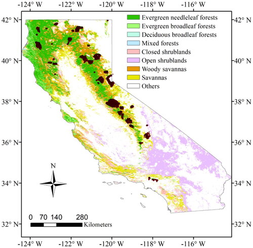
According to the MODIS land cover product, MCD12Q1, and International Geosphere–Biosphere Program (IGBP) classification scheme, evergreen needleleaf forests (ENF), woody savannas (WSA), and savannas (SAV) are the primary forest types across California. Figure 1 illustrates the spatial distribution of the forest types. The California boundary in the shapefile format was obtained from the website https://earthworks.stanford.edu/catalog/.

Figure 1. The forest types and forest AGB data across California; the dot points correspond to forest AGB at a 500 m spatial resolution obtained by aggregating the lidar-derived biomass at a 30 m spatial resolution.

2.2. Forest AGB data

Forest AGB data were initially derived from field measurements and airborne lidar data (Figure 1) and used to train the AGB model and validate the accuracy of the estimated AGB. They had accuracy as high as the field measurements and matched remotely sensed data better in spatial resolution than field plots (Zolkos et al. 2013). Thus, they were ideal for calibrating remotely sensed data and evaluating the estimated AGB.

Two lidar-derived data sets of forest AGB were collected. Xu and Greenberg (2018) generated forest AGB estimates at a 30 m spatial resolution from field measurements and airborne lidar surveys throughout California between 2005 and 2014. The field data used in their study included California-wide forest inventory and analysis (FIA) data and the data set collected by the United States Department of Agriculture (USDA) forest service. The AGB estimates at a 30 m resolution were obtained from the distributed active archive center website at https://doi.org/10.3334/ORNLDAAC/1537. Dubayah et al. (2017) provided AGB estimates at a 30 m spatial resolution for Parker Tract and Hubbard Brook Experimental Forest sites, California, for the nominal year 2013, by combining the field data and airborne lidar data collected by the Leica ALS70 sensor, which could be retrieved from https://doi.org/10.3334/ORNLDAAC/1523.

To be consistent with satellite-derived data in the following section, we aggregated both data sets at 30 m resolution to the 500 m by average (Figure 1). The aggregated AGB data were then randomly resampled with a geographic distance larger than 1 km from each other, generating 3671 reference AGB samples used for AGB modeling and accuracy evaluation (Liu et al. 2020). According to the statistics for the corresponding AGB values at a 500 m spatial resolution, generated reference samples ranged from 0.19 to 1616.32 Mg/ha, with an average and standard deviation of 285.70 and 229.71 Mg/ha respectively.

2.3. Satellite-derived data products

Due to their high quality and long time series, MODIS data products have been widely used in vegetation and environmental studies (Pastor-Guzman et al. 2018; Notarnicola 2020). We selected the MODIS data in this study because they have the eight-day temporal resolution and are dense in time series. Previous studies have proposed the correlations of the SR, LAI, the fraction of absorbed photosynthetically active radiation (FAPAR), GPP, and the canopy height (CH) with forest AGB (Muukkonen et al. 2006; Macdonald et al. 2012; Song et al. 2018; Pandey et al. 2019; Armstrong et al. 2020; Knapp et al. 2020). Hence, this study included the MODIS SR (MOD09A1), the LAI/FAPAR (MCD15A2), and GPP (MOD17A2) to estimate forest AGB.

All the MODIS data products were downloaded from NASA’s Land Processes Distributed Active Archive Center (https://lpdaac.usgs.gov/) and then reprojected from the sinusoidal projection to a geographic coordinate system using the nearest neighbor method. Table 1 tabulates the details about these MODIS products. Each product had an 8-day temporal resolution, and we extracted all 46 features within the year corresponding to the reference AGB samples collected.

Table 1. The data sets of the MODIS data products used for AGB estimation.

Product	Layers	Spatial resolution	Temporal resolution	Reference
MOD09A1	Surface reflectance bands 1–7	500 m	8 days	Vermote et al. (1997; 2002)
MCD15A2	LAI and FAPAR	500 m	8 days	Myneni et al. (2002; 2015)
MOD17A2	GPP	500 m	8 days	Running et al. (2015) and Zhao et al. (2005)

In addition to the MODIS data products, the forest canopy height was incorporated as a predictor due to its good correlations with forest AGB (Wang et al. 2013; Knapp et al. 2020). This work selected the global forest canopy height map produced by Simard et al. (Simard et al. 2011) from the Geoscience Laser Altimeter System (GLAS) data. We resampled the 1 km data to a 500 m spatial resolution using the nearest neighbor method to be consistent with other satellite-derived products.

2.4. Extracting temporal features from MODIS data products

To explore whether and how temporal information could enable accurate estimates of forest AGB, we developed four methods to extract temporal information from satellite-derived data products for modeling forest AGB. The AAF method included all annual features for the AGB estimation. The second method selected important features from annual time-series data based on the SCC criterion. Only features correlated with forest AGB larger than the mean correlation of features with forest AGB across the year were included. This method was independent of the AGB modeling algorithms used. The third approach utilized seasonal information for AGB estimation. The seasonal average and principal component analysis (PCA) components (SAP) of time-series data covering a specific season were employed for each season to estimate forest AGB. The PCA created new uncorrelated variables from the seasonal time-series features that might be highly correlated, which could enhance computational efficiency and minimize information loss (Li et al. 2008). The last method used phenological characteristic parameters (PCP) as the predictors of forest AGB. The Savitzky–Golay (S–G) method filtered annual MODIS data to extract phenological parameters from remotely sensed data. A dynamic threshold method proposed by Jonsson and Eklundh (Jonsson and Eklundh 2002) was then applied to the filtered annual time-series data for extracting the phenological parameters, including the start of the season (SOS), the end of the season (EOS), the length of the season (LOS), the peak of the season (POS), the minimum value of the left curve, the minimum value of the right curve, the slope of the SOS, the slope of the EOS, the amplitude of the season, and the cumulative value over the growing season (Zeng et al. 2011; Clement et al. 2013; Michele et al. 2014; Potapov et al. 2021). The SOS refers to the date when vegetation begins to grow, and the EOS refers to the date when vegetation photosynthesis begins to decline rapidly; the LOS refers to the period from the SOS to the EOS in days. We first conducted a pixel-by-pixel analysis and extracted the maximum value of the annual time series as the POS to determine these parameters. The SOS was defined as the point when the base level (the minimum value of the left curve) increased by 20% of the distance between the base level and the maximum value (Delbart et al. 2006; Van Leeuwen 2008; White et al. 2009; Michele et al. 2014). Similarly, the EOS was detected when the value of the curve dropped below the base level (the minimum value of the right curve) plus 20% of the amplitude (Meroni et al. 2014; Michele et al. 2014).

Among the above four methods, the SAP had four results corresponding to spring, summer, autumn, and winter. The optimal result that achieved the highest R-squared (R²) and lowest root-mean-squared error (RMSE) values was taken as the seasonal result compared to the three other methods. To investigate the potential of MODIS data products for forest AGB estimation, we applied the four methods to each of the 10 MODIS layers listed in Table 1: the 7 SR layers (bands 1–7), the LAI, the FAPAR, and the GPP. In addition, we examined the accuracy of AGB estimates by combining several satellite-derived data products and considered eight scenarios: (1) the combination of the LAI and the CH (LAI–CH); (2) the combination of the FAPAR and the CH (FAPAR–CH); (3) the combination of the GPP and the CH (GPP–CH); (4) the combination of MODIS SR bands 1, 4, and 6; (5) the combination of MODIS SR bands 1, 4, and 6, and the CH (SR–CH); (6) the combination of the LAI, FAPAR, and GPP (LFG); (7) the combination of the LAI, FAPAR, GPP, and CH (LFG–CH); (8) the combination of MODIS SR bands 1, 4, 6, and LFG–CH (Table 2). The surface reflectance data for bands 1, 4, and 6 were considered because the initial results indicated that these three SR bands resulted in the accurate estimation of forest AGB.

Table 2. The temporal features used for modeling AGB under 18 scenarios.

Scenarios	Name	Layers used
Individual layer	Band 1	MODIS SR band 1
	Band 2	MODIS SR band 2
	Band 3	MODIS SR band 3
	Band 4	MODIS SR band 4
	Band 5	MODIS SR band 5
	Band 6	MODIS SR band 6
	Band 7	MODIS SR band 7
	LAI	MODIS LAI
	FAPAR	MODIS FAPAR
	GPP	MODIS GPP
Combination of layers	LAI–CH	MODIS LAI and CH
	FAPAR–CH	MODIS FAPAR and CH
	GPP–CH	MODIS GPP and CH
	SR	MODIS SR bands 1, 4, and 6
	SR–CH	MODIS SR bands 1, 4, and 6 and CH
	LFG	MODIS LAI, FAPAR, and GPP
	LFG–CH	MODIS LAI, FAPAR, GPP, and CH
	All	MODIS SR bands 1, 4, and 6; LAI; FAPAR; GPP; and CH

2.5. AGB modeling algorithm

Ensemble machine learning algorithms are insensitive to outliers and achieve high accuracy in many fields (Zhang et al. 2022b). Random forest (RF) is the most extensively used tree-based ensemble algorithm (Breiman 2001). Some studies have suggested that boosting ensemble algorithms, such as gradient boosting machine (GBM) and CatBoost, can outperform RF and have a higher accuracy in predicting forest AGB than random forest (Zhang et al. 2020). Studies have recently reported that XGBoost is excellent at predicting PM2.5 concentrations, mapping plant species diversity, and estimating forest biomass (Zamani Joharestani et al. 2019; Li et al. 2020; Luo et al. 2021). Therefore, we selected the XGBoost algorithm for estimating forest aboveground biomass from satellite-derived time-series data in this study.

The XGBoost algorithm, proposed by Chen et al. (2016), is an improved version of the GBM algorithm. It is a scalable tree-boosting system that implements parallel preprocessing at the node level, making it faster than the GBM algorithm. It also includes regularization techniques to reduce overfitting. The primary hyperparameters of XGBoost included the maximum depth of the tree (max_depth), the minimum sample weight in leaf nodes (min_child_weight), the minimum value of the loss reduction required for the leaf nodes to the branch (gamma), the learning rate to prevent overfitting (learning_rate), the proportion of each tree randomly sampled (subsample), and the proportion of the number of columns randomly sampled per tree (colsample_bytree), which were optimized by the grid search method (Zhang et al. 2020; Zhang et al. 2022c) and implemented using python library xgboost.

2.6. Accuracy assessment

We used the five-fold cross-validation (CV) method to evaluate the accuracy of AGB estimates (Zhang et al. 2021). The 5-fold CV was repeated 10 times, generating 50 training and testing data sets. For each of the 50 data sets, the training data were used for AGB modeling, and the testing data were employed to assess the accuracy of AGB predictions. The evaluation metrics included R², RMSE, and bias (Zhang et al. 2020).

3. Results

3.1. Estimated forest AGB based on annual features extracted from different data products

We calculated the evaluation metrics achieved using the AAF method and the XGBoost algorithm under 18 scenarios (Figure 2). The most accurate estimation was provided by combining MODIS SR bands 1, 4, and 6 with the LAI, FAPAR, GPP, and CH, with an R² of 0.60 and an RMSE of 145.37 Mg/ha, followed by annual SR bands 1, 4, and 6 and the CH with an R² of 0.58 and an RMSE of 147.58 Mg/ha. In contrast, the estimated forest AGB had a lower degree of accuracy under the LAI (average R² of 0.44, RMSE of 172.01 Mg/ha, and bias of −0.32 Mg/ha), band 2 (average R² of 0.44, RMSE of 170.68 Mg/ha, and bias of −1.26 Mg/ha), and band 5 (average R² of 0.44, RMSE of 171.92 Mg/ha, and bias of −2.39 Mg/ha) scenarios. Comparing the results obtained based on the 10 individual layers revealed that MODIS band 4 outperformed the other scenarios, with an achieved average R² of 0.55, RMSE of 153.41 Mg/ha, and bias of −0.98 Mg/ha. Bands 1 and 6 also provided results comparable to MODIS band 4, with an R² higher than 0.50. The GPP, with an average R² of 0.49, RMSE of 163.65 Mg/ha, and bias of 0.28 Mg/ha, provided a more accurate AGB prediction than the LAI and FAPAR.

Figure 2. The accuracy of forest AGB estimated using the annual time-series data under the 18 scenarios; (a), (b), and (c) respectively represent the average R², RMSE, and bias values achieved by the AGB models developed under the 18 scenarios listed in Table 2.

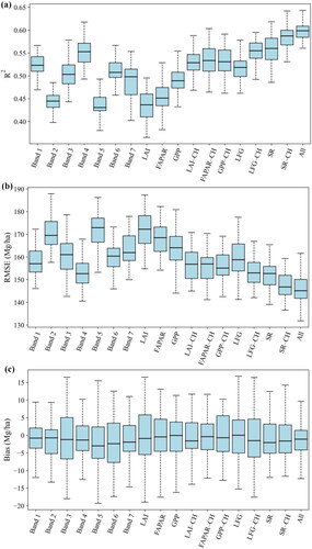
The LFG provided the least accurate estimation of forest AGB among the eight combination scenarios. Including the forest canopy height remarkably enhanced AGB prediction, as shown in Figure 2, which revealed the excellent correlation between the CH and biomass. The combination of the forest canopy height with the surface reflectance bands 1, 4, and 6 outweighed the prediction accuracy of the other combination scenarios. It also produced results comparable to those of the models built with all the data sets used in this study, indicating the potential of the SR–CH scenario to predict forest AGB. These results were also obtained when the SCC, PCP, and SAP methods were employed to extract time-series information (Figures 3 and 4).

Figure 3. The accuracy of forest AGB estimated using the seasonal time-series data under the 10 scenarios; (a), (b), and (c) respectively represent the seasonal R², RMSE, and bias values achieved by the AGB models developed under the 18 scenarios; the error bars show the 95% confidence intervals.

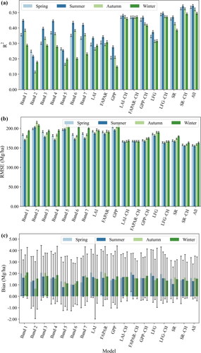
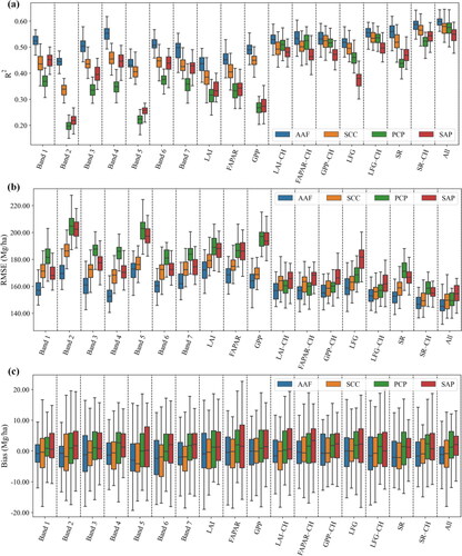
Figure 4. The accuracy of the forest AGB estimated using the temporal features selected by the AAF, SCC, PCP, and SAP methods; (a), (b), and (c) respectively represent R², RMSE, and bias values achieved under the 18 scenarios; the error bars show the 95% confidence intervals.

3.2. Contribution of seasonal time-series data to AGB estimation

According to Figure 3, the AGB predictions based on the summer data were more accurate than those based on the spring, autumn, and winter seasons, except for bands 2 and 5, with R² values ranging from 0.28 to 0.54 and RMSE values varying from 153.10 to 194.99 Mg/ha. The advantage of using the summer data for AGB estimation was more noticeable for bands 1, 4, and 6 than for the other bands. In contrast, the spring data provided more accurate estimates than the three other seasons for bands 2 and 5. Averaging the evaluation metrics obtained under 10 individual scenarios, we found that the summer data still provided more accurate AGB predictions, with an R² value of 0.36 and an RMSE of 183.28 Mg/ha. The average results of the eight combination scenarios showed that the summer data led to an average R² of 0.48, RMSE of 164.81 Mg/ha, and bias of 1.55 Mg/ha.

The AGB estimates based on the summer data were taken as the SAP results because of their high accuracy compared with the AAF, SCC, and PCP methods. Despite the higher degree of prediction accuracy obtained by the summer data, using MODIS data covering only one season could not provide reasonable estimates for forest AGB (Figures 3 and 4).

3.3. Impact of different methods and their extracted features on AGB estimation

The AAF provided the most accurate forest AGB estimates among the four methods used to extract temporal features from MODIS data (Figure 4). The SCC-based AGB estimates were close to the results obtained using the annual time-series data. The average R² value of the 10 individual scenarios using the SCC was 0.42, compared to an R² value of 0.49 achieved using the AAF method. Under the eight combination scenarios, the average R² value was 0.53 for the SCC method and 0.55 for the AAF, and the average RMSE was 157.54 Mg/ha for the SCC and 153.39 Mg/ha for the AAF method.

Furthermore, the results demonstrated that the predictions based on the PCP and SAP methods were worse than those determined by the AAF and SSC methods (Figure 4). The PCP approach led to a higher decrease in R² and an increase in the RMSE values relative to the results achieved by the AAF method than the SAP method under the 10 individual scenarios. These results indicated that the selected temporal features could be more effective in estimating forest AGB, and using seasonal or growing season features directly might not be an optimal choice for improving AGB estimation, as reported in previous studies. Under the LAI–CH, FAPAR–CH, GPP–CH, LFG, and LFG–CH scenarios, the PCP method provided more accurate results than the SAP approach, implying the capability of vegetation phenology for the retrieval of biomass (Duparc et al. 2013; Gwenzi et al. 2017).

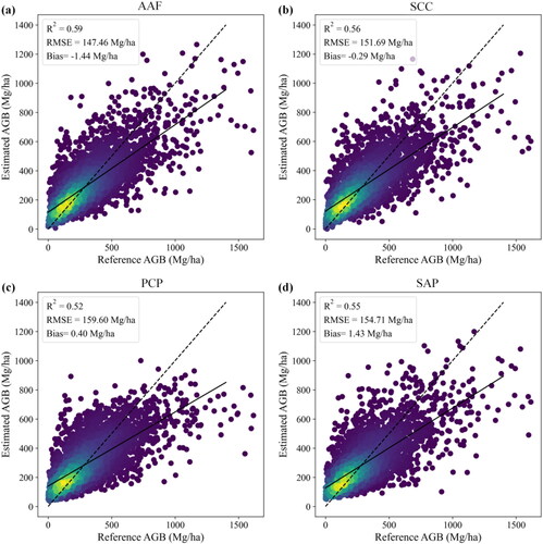
According to Figure 4, the PCP and SAP methods had overall positive biases, while the AAF and SSC methods had negative biases, indicating that the PCP and SAP methods generally underestimated forest AGB, but the AAF and SSC overestimated it to some degree. However, the scatter density plots of the reference AGB versus the estimated one indicated that forest AGB was overestimated at low values and underestimated at high values, independent of the methods employed to extract the temporal features from the MODIS data (see Figure 5). Among the four methods, the SCC estimated AGB with the least bias values, indicating that it could effectively identify essential predictor variables of forest AGB by performing feature selection, could avoid the curse dimensionality, and could remove unnecessary features from the one-year time-series data (Luo et al. 2021).

Figure 5. The density scatter plots of the reference AGB versus the AGB estimated by the AAF, SCC, PCP, and SAP methods and the five-fold cross-validation.

Despite the observed differences in the accuracy of the forest AGB estimates using features extracted by the four methods, a combination of the MODIS layers enhanced the accuracy of AGB estimation relative to the results achieved by using single indicators (see Figures 2 and 4).

3.4. Spatial distribution of estimated forest AGB in California

On the basis of the combined MODIS SR bands 1, 4, and 6 and the CH data, we mapped forest AGB using the AAF, SCC, PCP, and SAP methods and the XGBoost algorithm. Figure 6 shows the results. The forest AGB maps obtained using the AAF and SCC methods were basically consistent. The PCP and SAP methods led to higher AGB predictions in shrublands than the AAF and SCC methods. The AGB estimated based on the SAP was even higher than 200 Mg/ha in open shrublands, which indicated the severe overestimation of AGB in low biomass regions.

Figure 6. The spatial distribution of the forest AGB in 2013 estimated by the AAF, SCC, PCP, and SAP methods and the XGBoost algorithm based on the SR–CH data.

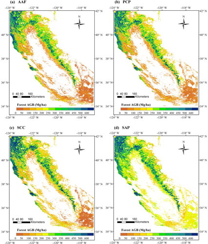
In contrast, the AGB values of evergreen needleleaf forests determined by the SAP and PCP methods were smaller than those predicted using the AAF and SCC methods (Figure 6). Roughly 14.73% of the forest pixels had an estimated AGB of less than 50 Mg/ha, while the proportions were 9.31% and 7.55% for the SCC and PCP methods. According to the SAP-based biomass map, all the forest pixels had an AGB value higher than 50 Mg/ha. Almost 44.32% of the forest pixels had estimated AGB values ranging from 50 to 200 Mg/ha, while 48.27% and 53.78% of the forest pixels were located in the ranges according to the results obtained by the SCC and PCP methods respectively. According to the results estimated by the SAP method, only 30.69% of the forest pixels had a forest AGB, and 28.77% had an estimated AGB of 200–250 Mg/ha.

4. Discussion

This study examined the performance of the different temporal features extracted from MODIS data products in estimating forest AGB. The results indicated that the green band, red band, and shortwave infrared were sensitive to forest AGB, agreeing with previous works (Muukkonen and Heiskanen 2005; Mutanga et al. 2012; Nandy et al. 2017; Dube et al. 2018). Band 4 provided the most abundant information for AGB prediction among the seven MODIS SR bands. Although some studies agreed that the green band reflectance was suitable for predicting biomass, more works found that the shortwave infrared reflectance was highly correlated with biomass (Molinier et al. 2016; Nandy et al. 2017). However, the results of this study showed that the green band reflectance was more useful than the shortwave infrared and near-infrared bands. Thus, green band reflectance is necessary for forest AGB estimation in future studies. Further investigation should be conducted to determine whether and under which conditions the findings are established or applied to different spatial resolutions.

Regarding the four analytical methods to extract the features of annual MODIS data, this study revealed that the AAF and SCC methods led to similar results and provided a more accurate estimation of forest AGB than the other methods. Employing seasonal data or growing season data (phenological information) always produced the worst results, implying the limitations of estimating forest AGB using the data of a specific season. Published studies exploring the contribution of seasonal or time-series data have commonly utilized summer or autumn data or only one image acquired in a specific season (Zhu and Liu 2015; Nguyen et al. 2020), mainly ignoring the contribution of information from the other seasons. Therefore, our results highlighted that spring or winter features extracted from indicators might play a dominant role in AGB estimation; moreover, a few features from the other seasons were also indispensable for accurately estimating forest AGB. Performing feature selection to extract critical features from annual time-series data rather than simply using seasonal or growing season data might be more effective in taking advantage of temporal features to enhance the accuracy of AGB prediction. In addition, we extracted quantile statistics of the MODIS SR, LAI, FAPAR, and GPP and combined these statistical predictors for AGB estimation, similar to most published studies. The experimental results were poorer than ours, which also confirmed the significance of this study.

Satellite-derived time-series data can suffer from cloud cover, atmospheric variability, and aerosol scattering. For this reason, some studies have utilized smoothing or reconstruction techniques to improve the temporal trajectories of various remotely sensed data and then used the smoothed data instead of the original time-series data to estimate forest AGB. Their results showed that the AGB models developed using the smoothed time-series data substantially outperformed those based on the original data (Urbazaev et al. 2016; Li et al. 2018). This study preprocessed the raw data utilizing an S–G filter (Pan et al. 2015) and used the smoothed data instead of the original data to predict forest AGB based on satellite-derived data products. Nevertheless, we found that the results under the four time-series scenarios were consistent with those determined using raw time-series data without preprocessing, which, to some extent, indicated the robustness of our analytical methods.

Although the AAF method produced the most accurate results, about 60% of variations were explained by combining annual time-series data, leaving much room to improve. This study obtained large RMSE values partly because some training samples had AGB values higher than 500 Mg/ha, which was far beyond the capability of optical imagery for estimation, and RMSE was quite sensitive to the data set distribution and outliers. The forest AGB estimated herein was higher than some published results (Zhang et al. 2014a; Gonzalez et al. 2015), which might be because we used lidar-derived forest AGB data to calibrate satellite data sets, and some training samples were located in dense forests and had higher AGB values (see Figure 1). Nevertheless, the results of this study confirmed that by exploiting temporal information from multiple satellite-derived data products, the accuracy of AGB prediction could be markedly improved. Future studies should consider more advanced algorithms, such as deep learning algorithms, to estimate forest AGB using time-series data to further enhance forest AGB estimation.

The main objective of this study was to improve the accuracy of AGB estimates by exploiting temporal information. To this end, we conducted experiments with MODIS data products at the 500 m spatial resolution because of their high temporal resolutions. Although ignored in this study, spatial information could improve the AGB predictions (Zhang et al. 2019). Some recent studies combined Landsat and MODIS data to generate time-series data with high spatial and temporal resolutions (Gevaert and García-Haro 2015; Zhang et al. 2022a). Using these generated data could improve the AGB prediction in theory and should be explored in future studies (Yang et al. 2022). In addition, the SAR data, topographical data, climatic factors, land surface temperature, and soil moisture should be included to further improve the prediction accuracy of forest AGB (Zhang et al. 2019; Jiang et al. 2021).

5. Conclusions

This study thoroughly investigated whether and how the temporal information of multiple satellite-derived data could be beneficial for forest AGB estimation. AAF, SCC, PCP, and SAP methods were developed to extract temporal features from the MODIS SR, LAI, FAPAR, and GPP data. The results of this study revealed that the AAF produced the most accurate estimation of forest AGB among the four analytical methods, followed by the SCC. The summer features of the reflectance data and biophysical variables, including the LAI, FAPAR, and GPP, played a more crucial role in biomass estimation than the other seasons. However, the seasonal results were less accurate than the SCC and AAF methods, indicating that the satellite data covering a specific season might not be enough to predict the forest AGB accurately. The SCC-based AGB estimation had the slightest bias, possibly due to removing redundant predictors within a year by performing feature selection.

In addition, the inclusion of the forest canopy height in the MODIS time-series data improved the accuracy of AGB estimation, so it was applied to the four methods. Combining the annual time-series SR data for bands 1, 4, and 6 with the CH could provide an accurate estimation of forest AGB, with an average R² of 0.58 and an RMSE of 147.58 Mg/ha, close to the results achieved by combining MODIS SR bands 1, 4, and 6 with the LAI, FAPAR, GPP, and CH with an R² of 0.60 and an RMSE of 145.37 Mg/ha. This highlights the necessity of utilizing annual SR time-series data in future studies. Last but not least, more advanced algorithms for modeling the forest AGB should be developed to further enhance the accuracy of estimated results.

Data availability

The data that support the findings of this study are available on request from the corresponding author.

Disclosure statement

The authors report that there are no competing interests to declare.

Additional information

Funding

National Natural Science Foundation of China (Grant No. 41801347).

References

- Ahmed R, Siqueira P, Hensley S. 2013. A study of forest biomass estimates from Lidar in the northern temperate forests of New England. Remote Sens Environ. 130:121–135.
- Allen RJ, Luptowitz R. 2017. El niño-like teleconnection increases California precipitation in response to warming. Nat Commun. 8(1):16055.
- Amini J, Sumantyo JTS. 2009. Employing a method on sar and optical images for forest biomass estimation. IEEE Trans Geosci Remote Sens. 47(12):4020–4026.
- Armstrong AH, Huth A, Osmanoglu B, Sun G, Ranson KJ, Fischer R. 2020. A multi-scaled analysis of forest structure using individual-based modeling in a Costa Rican rainforest. Ecol Modell. 433:109226.
- Baccini A, Goetz SJ, Walker WS, Laporte NT, Sun M, Sulla-Menashe D, Hackler J, Beck PSA, Dubayah R, Friedl MA, et al. 2012. Estimated carbon dioxide emissions from tropical deforestation improved by carbon-density maps. Nat Clim Change. 2(3):182–185.
- Breiman L. 2001. Random forests. Mach Learn. 45(1):5–32.
- Chen TQ, Guestrin C, Assoc Comp M. 2016. Xgboost: a scalable tree boosting system.
- Clement A, Anja K, Matteo M, Francesco V. 2013. Phenological metrics derived over the European continent from ndvi3g data and modis time series. Remote Sens. 6(1):257–257.
- Cramer JC. 1998. Population growth and air quality in California. Demography. 35(1):45–56.
- Cramer JC, Cheney RP. 2000. Lost in the ozone: population growth and ozone in California. Popul Environ. 21(3):315–338.
- Delbart N, Le Toan T, Kergoat L, Fedotova V. 2006. Remote sensing of spring phenology in boreal regions: a free of snow-effect method using noaa-avhrr and spot-vgt data (1982-2004). Remote Sens Environ. 101(1):52–62.
- Dhillon RS, Von Wuehlisch G. 2013. Mitigation of global warming through renewable biomass. Biomass Bioenergy. 48:75–89.
- Dubayah RO, Swatantran A, Huang W, Duncanson L, Tang H, Johnson K, Dunne JO, Hurtt GC. 2017. Cms: lidar-derived biomass, canopy height and cover, Sonoma County, California, 2013. ORNL Distributed Active Archive Center.
- Dube T, Gara TW, Mutanga O, Sibanda M, Shoko C, Murwira A, Masocha M, Ndaimani H, Hatendi CM. 2018. Estimating forest standing biomass in Savanna woodlands as an indicator of forest productivity using the new generation worldview-2 sensor. Geocarto Int. 33(2):178–188.
- Duffy PB, Bonfils C, Lobell D. 2007. Interpreting recent temperature trends in California. Eos Trans AGU. 88(41):409–410.
- Duparc A, Redjadj C, Viard-Cretat F, Lavorel S, Austrheim G, Loison A. 2013. Co-variation between plant above-ground biomass and phenology in sub-alpine grasslands. Appl Veg Sci. 16(2):305–316.
- Fettig CJ, Mortenson LA, Bulaon BM, Foulk PB. 2019. Tree mortality following drought in the central and southern Sierra Nevada, California, U.S. For Ecol Manage. 432:164–178.
- Gershunov A, Shulgina T, Clemesha RES, Guirguis K, Pierce DW, Dettinger MD, Lavers DA, Cayan DR, Polade SD, Kalansky J, et al. 2019. Precipitation regime change in western North America: the role of atmospheric rivers. Sci Rep. 9(1):9944.
- Gevaert CM, García-Haro FJ. 2015. A comparison of starfm and an unmixing-based algorithm for landsat and MODIS data fusion. Remote Sens Environ. 156:34–44.
- Gonzalez P, Battles JJ, Collins BM, Robards T, Saah DS. 2015. Aboveground live carbon stock changes of California Wildland ecosystems, 2001–2010. For Ecol Manage. 348:68–77.
- Gwenzi D, Helmer EH, Zhu X, Lefsky MA, Marcano-Vega H. 2017. Predictions of tropical forest biomass and biomass growth based on stand height or canopy area are improved by landsat-scale phenology across Puerto Rico and the US Virgin Islands. Remote Sens. 9(2):123.
- Hayashi M, Motohka T, Sawada Y. 2019. Aboveground biomass mapping using alos-2/palsar-2 time-series images for Borneo’s forest. IEEE J Sel Top Appl Earth Observ Remote Sens. 12(12):5167–5177.
- Jiang F, Kutia M, Ma K, Chen S, Long J, Sun H. 2021. Estimating the aboveground biomass of Coniferous Forest in Northeast China using spectral variables, land surface temperature and soil moisture. Sci Total Environ. 785:147335.
- Jonsson P, Eklundh L. 2002. Seasonality extraction by function fitting to time-series of satellite sensor data. IEEE Trans Geosci Remote Sens. 40(8):1824–1832.
- Kamir E, Waldner F, Hochman Z. 2020. Estimating wheat yields in Australia using climate records, satellite image time series and machine learning methods. ISPRS J Photogramm Remote Sens. 160:124–135.
- Keeling HC, Phillips OL. 2007. The global relationship between forest productivity and biomass. Glob Ecol Biogeogr. 16(5):618–631.
- Knapp N, Fischer R, Cazcarra-Bes V, Huth A. 2020. Structure metrics to generalize biomass estimation from lidar across forest types from different continents. Remote Sens Environ. 237:111597.
- Le Maire G, Marsden C, Nouvellon Y, Grinand C, Hakamada R, Stape J-L, Laclau J-P. 2011. Modis NDVI time-series allow the monitoring of eucalyptus plantation biomass. Remote Sens Environ. 115(10):2613–2625.
- Le Toan T, Quegan S, Davidson MWJ, Balzter H, Paillou P, Papathanassiou K, Plummer S, Rocca F, Saatchi S, Shugart H, et al. 2011. The biomass mission: mapping global forest biomass to better understand the terrestrial carbon cycle. Remote Sens Environ. 115(11):2850–2860.
- Li XJ, Du HQ, Mao FJ, Zhou GM, Chen L, Xing LQ, Fan WL, Xu XJ, Liu YL, Cui L, et al. 2018. Estimating bamboo forest aboveground biomass using ENKF-assimilated modis lai spatiotemporal data and machine learning algorithms. Agric For Meteorol. 256-257:445–457.
- Li Y, Andersen H-E, Mcgaughey R. 2008. A comparison of statistical methods for estimating forest biomass from light detection and ranging data. Western J Appl For. 23(4):223–231.
- Li Y, Li M, Li C, Liu Z. 2020. Forest aboveground biomass estimation using landsat 8 and sentinel-1a data with machine learning algorithms. Sci Rep. 10(1):9952.
- Liu H, Gong P, Wang J, Clinton N, Bai Y, Liang S. 2020. Annual dynamics of global land cover and its long-term changes from 1982 to 2015. Earth Syst Sci Data. 12(2):1217–1243.
- Liu L, Peng D, Wang Z, Hu Y. 2014. Improving artificial forest biomass estimates using afforestation age information from time series landsat stacks. Environ Monit Assess. 186(11):7293–7306.
- Luo M, Wang Y, Xie Y, Zhou L, Qiao J, Qiu S, Sun Y. 2021. Combination of feature selection and catboost for prediction: the first application to the estimation of aboveground biomass. Forests. 12(2):216.
- Macdonald RL, Burke JM, Chen HYH, Prepas EE. 2012. Relationship between aboveground biomass and percent cover of ground vegetation in Canadian boreal plain riparian forests. For Sci. 58(1):47–53.
- Machwitz M, Gessner U, Conrad C, Falk U, Richters J, Dech S. 2015. Modelling the gross primary productivity of West Africa with the regional biomass model rbm+, using optimized 250m modis fpar and fractional vegetation cover information. Int J Appl Earth Obs Geoinf. 43:177–194.
- Malhi Y, Doughty C, Galbraith D. 2011. The allocation of ecosystem net primary productivity in tropical forests. Phil Trans R Soc B. 366(1582):3225–3245.
- Mann ME, Gleick PH. 2015. Climate change and California drought in the 21st century. Proc Natl Acad Sci U S A. 112(13):3858–3859.
- Mcbride JR, Laćan I. 2018. The impact of climate-change induced temperature increases on the suitability of street tree species in California (USA) cities. Urban For Urban Green. 34:348–356.
- Mcintyre PJ, Thorne JH, Dolanc CR, Flint AL, Flint LE, Kelly M, Ackerly DD. 2015. Twentieth-century shifts in forest structure in California: denser forests, smaller trees, and increased dominance of oaks. Proc Natl Acad Sci U S A. 112(5):1458–1463.
- Meroni M, Verstraete MM, Rembold F, Urbano F, Kayitakire F. 2014. A phenology-based method to derive biomass production anomalies for food security monitoring in the horn of Africa. Int J Remote Sens. 35(7):2472–2492.
- Meroni M, Rembold F, Verstraete M, Gommes R, Schucknecht A, Beye G. 2014. Investigating the relationship between the inter-annual variability of satellite-derived vegetation phenology and a proxy of biomass production in the Sahel. Remote Sens. 6(6):5868–5884.
- Minnich RA, Barbour MG, Burk JH, Sosa-Ramírez J. 2000. Californian mixed-conifer forests under unmanaged fire regimes in the Sierra San Pedro Mártir, Baja California, Mexico. J Biogeogr. 27(1):105–129.
- Mitchard E, Saatchi S, Baccini A, Asner G, Goetz S, Harris N, Brown S. 2013. Uncertainty in the spatial distribution of tropical forest biomass: a comparison of pan-tropical maps. Carbon Balance Manag. 8(1):10.
- Mitchard ETA. 2018. The tropical forest carbon cycle and climate change. Nature. 559(7715):527–534.
- Molinier M, López-Sánchez CA, Toivanen T, Korpela I, Corral-Rivas JJ, Tergujeff R, Häme T. 2016. Relasphone—mobile and participative in situ forest biomass measurements supporting satellite image mapping. Remote Sens. 8(10):869.
- Moradi F, Sadeghi SMM, Heidarlou HB, Deljouei A, Boshkar E, Borz SA. 2022. Above-ground biomass estimation in a mediterranean sparse coppice oak forest using Sentinel-2 data.
- Mutanga O, Adam E, Cho MA. 2012. High density biomass estimation for wetland vegetation using worldview-2 imagery and random forest regression algorithm. Int J Appl Earth Obs Geoinf. 18:399–406.
- Muukkonen P, Heiskanen J. 2005. Estimating biomass for boreal forests using aster satellite data combined with standwise forest inventory data. Remote Sens Environ. 99(4):434–447.
- Muukkonen P, Makipaa R, Laiho R, Minkkinen K, Vasander H, Finer L. 2006. Relationship between biomass and percentage cover in understorey vegetation of boreal coniferous forests. Silva Fenn. 40(2):231–245.
- Nandy S, Singh R, Ghosh S, Watham T, Kushwaha SPS, Kumar AS, Dadhwal VK. 2017. Neural network-based modelling for forest biomass assessment. Carbon Manage. 8(4):305–317.
- Nguyen TH, Jones S, Soto-Berelov M, Haywood A, Hislop S. 2020. Landsat time-series for estimating forest aboveground biomass and its dynamics across space and time: a review. Remote Sens. 12(1):98.
- Notarnicola C. 2020. Hotspots of snow cover changes in global mountain regions over 2000-2018. Remote Sens Environ. 243:111781.
- Nuthammachot N, Askar A, Stratoulias D, Wicaksono P. 2022. Combined use of sentinel-1 and sentinel-2 data for improving above-ground biomass estimation. Geocarto Int. 37(2):366–376.
- Pan Z, Huang J, Zhou Q, Wang L, Cheng Y, Zhang H, Blackburn GA, Yan J, Liu J. 2015. Mapping crop phenology using ndvi time-series derived from hj-1 a/b data. Int J Appl Earth Obs Geoinf. 34:188–197.
- Pandey PC, Srivastava PK, Chetri T, Choudhary BK, Kumar P. 2019. Forest biomass estimation using remote sensing and field inventory: a case study of Tripura, India. Environ Monit Assess. 191(9):593.
- Pastor-Guzman J, Dash J, Atkinson PM. 2018. Remote sensing of mangrove forest phenology and its environmental drivers. Remote Sens Environ. 205:71–84.
- Pflugmacher D, Cohen WB, Kennedy RE, Yang Z. 2014. Using landsat-derived disturbance and recovery history and lidar to map forest biomass dynamics. Remote Sens Environ. 151:124–137.
- Polade SD, Gershunov A, Cayan DR, Dettinger MD, Pierce DW. 2017. Precipitation in a warming world: assessing projected hydro-climate changes in California and other mediterranean climate regions. Sci Rep. 7(1):10783.
- Potapov P, Li X, Hernandez-Serna A, Tyukavina A, Hansen MC, Kommareddy A, Pickens A, Turubanova S, Tang H, Silva CE, et al. 2021. Mapping global forest canopy height through integration of gedi and landsat data. Remote Sens Environ. 253:112165.
- Saatchi SS, Harris NL, Brown S, Lefsky M, Mitchard ETA, Salas W, Zutta BR, Buermann W, Lewis SL, Hagen S, et al. 2011. Benchmark map of forest carbon stocks in tropical regions across three continents. Proc Natl Acad Sci U S A. 108(24):9899–9904.
- Sanstad AH, Johnson H, Goldstein N, Franco G. 2011. Projecting long-run socioeconomic and demographic trends in California under the sres a2 and b1 scenarios. Clim Change. 109(S1):21–42.
- Sarker MLR, Nichol J, Iz HB, Ahmad BB, Rahman AA. 2013. Forest biomass estimation using texture measurements of high-resolution dual-polarization c-band sar data. IEEE Trans Geosci Remote Sens. 51(6):3371–3384.
- Simard M, Pinto N, Fisher JB, Baccini A. 2011. Mapping forest canopy height globally with spaceborne lidar. J Geophys Res. 116(G4):G04021.
- Sinha S, Jeganathan C, Sharma LK, Nathawat MS. 2015. A review of radar remote sensing for biomass estimation. Int J Environ Sci Technol. 12(5):1779–1792.
- Song C. 2012. Optical remote sensing of forest leaf area index and biomass. Prog Phys Geogr.
- Song X, Zeng X, Tian D. 2018. Allocation of forest net primary production varies by forest age and air temperature. Ecol Evol. 8(23):12163–12172.
- Stovall AEL, Shugart H, Yang X. 2019. Tree height explains mortality risk during an intense drought. Nat Commun. 10(1):4385.
- Struglia R, Winter PL. 2002. The role of population projections in environmental management. Environ Manage. 30(1):13–23.
- Sun G, Ranson KJ, Guo Z, Zhang Z, Montesano P, Kimes D. 2011. Forest biomass mapping from lidar and radar synergies. Remote Sens Environ. 115(11):2906–2916.
- Urbazaev M, Thiel C, Migliavacca M, Reichstein M, Rodriguez-Veiga P, Schmullius C. 2016. Improved multi-sensor satellite-based aboveground biomass estimation by selecting temporally stable forest inventory plots using ndvi time series. Forests. 7(12):169.
- Van Leeuwen WJD. 2008. Monitoring the effects of forest restoration treatments on post-fire vegetation recovery with modis multitemporal data. Sensors (Basel). 8(3):2017–2042.
- Wang X, Ouyang S, Sun OJ, Fang J. 2013. Forest biomass patterns across Northeast China are strongly shaped by forest height. For Ecol Manage. 293:149–160.
- White JC, Wulder MA, Hermosilla T, Coops NC, Hobart GW. 2017. A nationwide annual characterization of 25years of forest disturbance and recovery for Canada using landsat time series. Remote Sens Environ. 194:303–321.
- White MA, De Beurs KM, Didan K, Inouye DW, Richardson AD, Jensen OP, O'keefe J, Zhang G, Nemani RR, Van Leeuwen WJD, et al. 2009. Intercomparison, interpretation, and assessment of spring phenology in North America estimated from remote sensing for 1982-2006. Glob Change Biol. 15(10):2335–2359.
- Xu Q, Greenberg J. 2018. Lidar-derived aboveground biomass and uncertainty for California forests, 2005-2014. ORNL Distributed Active Archive Center.
- Yang B, Zhang Y, Mao X, Lv Y, Shi F, Li M. 2022. Mapping spatiotemporal changes in forest type and aboveground biomass from landsat long-term time-series analysis—a case study from Yaoluoping National Nature Reserve, Anhui province of Eastern China. Remote Sens. 14(12):2786.
- Yu Y, Saatchi S, Heath LS, Lapoint E, Myneni R, Knyazikhin Y. 2010. Regional distribution of forest height and biomass from multisensor data fusion. J Geophys Res. 115(G2):n/a–n/a.
- Zamani Joharestani M, Cao C, Ni X, Bashir B, Talebiesfandarani S. 2019. Pm2.5 prediction based on random forest, xgboost, and deep learning using multisource remote sensing data. Atmosphere. 10(7):373.
- Zeng H, Jia G, Epstein H. 2011. Recent changes in phenology over the northern high latitudes detected from multi-satellite data. Environ Res Lett. 6(4):045508–045518.
- Zhang G, Ganguly S, Nemani RR, White MA, Milesi C, Hashimoto H, Wang W, Saatchi S, Yu Y, Myneni RB. 2014a. Estimation of forest aboveground biomass in California using canopy height and leaf area index estimated from satellite data. Remote Sens Environ. 151(0):44–56.
- Zhang Y, Li W, Liang S. 2021. New metrics and the combinations for estimating forest biomass from glas data. IEEE J Sel Top Appl Earth Observ Remote Sens. 14:7830–7839.
- Zhang Y, Liang S, Sun G. 2014b. Forest biomass mapping of Northeastern China using glas and modis data. IEEE J Sel Top Appl Earth Observ Remote Sens. 7(1):140–152.
- Zhang Y, Liang S, Yang L. 2019. A review of regional and global gridded forest biomass datasets. Remote Sens. 11(23):2744.
- Zhang Y, Liu J, Liang S, Li M. 2022a. A new spatial–temporal depthwise separable convolutional fusion network for generating landsat 8-day surface reflectance time series over forest regions. Remote Sens. 14(9):2199.
- Zhang Y, Liu J, Shen W. 2022b. A review of ensemble learning algorithms used in remote sensing applications. Appl Sci. 12(17):8654.
- Zhang Y, Ma J, Liang S, Li X, Li M. 2020. An evaluation of eight machine learning regression algorithms for forest aboveground biomass estimation from multiple satellite data products. Remote Sens. 12(24):4015.
- Zhang Y, Ma J, Liang S, Li X, Liu J. 2022c. A stacking ensemble algorithm for improving the biases of forest aboveground biomass estimations from multiple remotely sensed datasets. GISci Remote Sens. 59(1):234–249.
- Zhu X, Liu D. 2015. Improving forest aboveground biomass estimation using seasonal landsat ndvi time-series. ISPRS J Photogramm Remote Sens. 102:222–231.
- Zolkos SG, Goetz SJ, Dubayah R. 2013. A meta-analysis of terrestrial aboveground biomass estimation using lidar remote sensing. Remote Sens Environ. 128:289–298.