Towards quantifying the relative tectonic activity in the Trans-Yamuna segment of NW Himalaya

Abstract

Owing to the increased availability of high-resolution satellite data and the rapid development of Geographic Information System (GIS) technology, the mapping of active faults and quantification of tectonic activity in inaccessible regions has exceedingly improved. We examined the tectonic activity in the Trans-Yamuna region of the NW Himalaya using geomorphic indices derived from a Digital Elevation Model (DEM). In addition, this study evaluates the sensitivity of four space-borne Digital Elevation Models (DEMs) with respect to TAN DEM-X (TerraSAR-X add-on for Digital Elevation Measurements). The Cartosat DEM, generated with a spatial resolution of 5 meters using state-of-the-art methods, demonstrated a reliable representation of topography. Geomorphic indices such as Asymmetry Factor (AF), Transverse Topography (TT), Hypsometric Integral (HI), Valley Floor width (Vf), Stream-length gradient index (SL), and Normalised steepness index (ksn) were computed for 41 sub-watersheds to determine the degree of tectonic activity. We infer that majority of the region is tectonically active, with upliftment continuing to occur in the north of the Main Boundary Thrust (MBT). Furthermore, the existence of mapped active faults north of the MBT further substantiates the fact that strain release is not only concentrated in the frontal Himalaya, but is distributed over a broader area above the decollement.

Keywords:

• Active faults
• earthquake hazard assessment
• geomorphic indices
• digital elevation model

1. Introduction

The Himalaya, which form the northern boundary of the Indian plate, is one of the most seismically active orogenic belt. It was formed during the Late Cretaceous-Early Paleogene by the collision-convergence of the Indian and Eurasian plates (Styron et al., 2010). This continued convergence over time has resulted in the formation of a large lateral zone of deformation extending 2500 kilometers, which has been accommodated by crustal shortening and has given rise to the major south-verging thrust systems (Gansser 1964; Seeber and Armbruster 1981; Tapponnier et al. 1982; Lyon-Caen and Molnar 1985; Taylor et al. 2003; Valdiya 2003). The principal thrusts are the Main Central Thrust (MCT), the Main Boundary Thrust (MBT) and the Himalayan Frontal Thrust (HFT). Each of these thrust systems further merge into the basal detachment fault, i.e. Main Himalayan Thrust (MHT) (Zhao et al. 1993; Pandey et al. 1995). According to geodetic measurements, the convergence rate across Nepal Himalaya ranges from 17.8 ± 0.5 to 20.5 ± 1 mm/yr (Bettinelli et al. 2006; Ader et al. 2012; Stevens and Avouac 2015) and across Northwest Himalaya ranges between 13.6 ± 1 to 14 ± 1 mm/yr (Banerjee and Bürgmann 2002; Kundu et al. 2014). For the Kumaon-Garhwal region of the Himalaya, the estimated plate convergence rate is 17.5 mm/yr (Banerjee and Bürgmann 2002; Jade et al. 2014; Yadav et al. 2019). The thrusting of the Eurasian plate over the Indian plate and locking along the MHT is the cause for heterogenous deformation rates that leads to the accumulation of high elastic energy along the plate boundary region. As a result, the HFT manifests into a zone of active deformation and associated uplift (Nakata 1989; Gautam et al. 2017). Consequently, the Himalayan Frontal zone with the maximum amount of tectonic activity has been extensively studied in India, Nepal and Bhutan (Wesnousky et al. 1999; Kumar et al. 2001; Lavé et al. 2005; Senthil et al. 2006; Kumar et al. 2010; Malik et al. 2010; Philip et al. 2012; Kumahara and Jayangondaperumal 2013; Sapkota et al. 2013; Bollinger et al. 2014; Le Roux-Mallouf et al. 2016; Hetényi et al. 2016; Jayangondaperumal et al. 2017).

However, we cannot eliminate the fact that several imbricate and out-of-sequence faults have developed in the hinterland as a result of the slip accommodation not reaching the frontal zone. Relatively, a minor amount of research has been undertaken in the hinterland regions. Therefore, the mapping and identification of active faults is significant not only in the frontal areas but also in the hinterland for determination of the earthquake potential of these zones (Oatney et al. 2001; Thakur et al. 2014; Philip et al. 2017; Arora et al. 2019). Several techniques, such as paleoseismic, geophysical, and morphotectonic studies using satellite image analysis, are employed worldwide to map and delineate the active faults. In mountain ranges, recent and active tectonics can be viewed as a major factor that contributes to rock uplifting; their present-day topography being the result of the interaction between tectonic and erosional processes (England and Molnar 1990; Valdiya 1993; Bishop 2007; Pérez-Peña et al. 2010; Rebai et al. 2013). Moreover, in tectonically active terrains, the landscape bears evidence of active faulting in the form of geomorphic markers (Burbank and Anderson 2011). Among the geomorphic markers, fluvial systems are the most sensitive features which have direct spatial and temporal relationship with changes in tectonic deformations (Holbrook and Schumm 1999; Snyder et al. 2000; Kirby and Whipple 2012). As a result, geomorphic indices and morphotectonic parameters can be used as reconnaissance tools to determine and quantify the amount of deformation in a tectonically active area. These parameters help in rapidly evaluating regional tectonic activity and can be easily extracted from topographic and aerial photographs (Hack 1973; Cox 1994; Pinter 2002).

Several studies involving morphotectonic indices have been successfully completed in various tectonically active areas around the world (Silva et al. 2003; El Hamdouni et al. 2008; Dehbozorgi et al. 2010; Gao et al. 2013; Hassen et al. 2014; Karabulut and Özdemir 2019; Zhang et al. 2019b; Khalifa et al. 2019; Buczek and Górnik 2020; Khalifa et al. 2021). Similarly, several researchers have utilized freely available global DEMs to conduct in-depth morphotectonic investigations on the Himalayan river systems (Singh and Jain 2009; Mahmood and Gloaguen 2012; Divyadarshini and Singh 2017; Kothyari et al. 2021; Luirei et al. 2022). For decades, researchers preferred topographic maps to generate high-resolution digital elevation models (DEMs) by digitization of contours, and relied on aerial photographs for mapping and delineation of geomorphic and tectonic features (Zevenbergen and Thorne 1987), which appeared time-exhaustive, labour intensive and expensive. In the last decade, the availability of high quality DEMs like the Shuttle Radar Topography Mission (SRTM with 90 m and 30 m), Advanced Spaceborne Thermal Emission and Refection Radiometer (ASTER) (version 3, 30 m), ALOS (Advanced Land Observing Satellite) PRISM (Panchromatic Remote-sensing Instrument for Stereo Mapping − 30 m and 12.5 m), and TanDEM-X (TerraSAR-X add-on for Digital Elevation Measurements) have opened up a new era in terrain mapping. On the other hand, state-of-the art instruments and methods in the form of Light Detection and Ranging (LiDAR), Unmanned Aerial Vehicles (UAV) using Structure from Motion (SFM) technologies and Synthetic Aperture Radar (SAR) data are extensively being utilized for fault mapping and high-resolution terrain mapping (Langridge et al. 2018; Guo et al. 2021; Liang et al. 2021). However, SAR, UAV and LiDAR comprises few limitations in generating high-resolution DEM over highly undulated terrain (Finley et al. 2021; Gao et al. 2021; Mukhamediev et al. 2021; Braun 2021). Given the foregoing, digital photogrammetry has emerged as a viable method for generating high-resolution DEMs from stereo pairs for terrain mapping.

Despite the fact that we have access to a large number of freely available DEMs, selecting the most appropriate DEM for a certain methodology remains a challenging task (De Vente et al. 2009). It is a well-known fact that DEM errors have a cumulative effect on the spatial indices obtained from them and have a detrimental impact on the accuracy of the model as a result of this (López 1997; Florinsky 1998; Vaze et al. 2010). The accuracy of a DEM is governed by factors such as the type and configuration of the equipment implemented for image retrieval, the methodology for DEM generation, and the topographic complexity of the landscape (Thompson et al. 2001; Fisher and Tate 2006; Nuth and Kääb 2011). According to Aguilar et al. (2005) topographic complexity is considered to be the most important factor for DEM accuracy. Thus, the Himalayan region, which is considered to be a highly rugged and complex terrain with dense vegetation and snow cover, demonstrates larger DEM errors. The incorporation of a DEM solely based on the global estimates of vertical accuracy for morphotectonic assessment, especially at catchment scale in a highly undulating terrain, will produce biased results. In this context, several researchers have resorted to digital photogrammetric techniques with or without the use of Ground Control Points (GCPs) to generate high resolution DEMs as per their requirements (Tateishi and Akutsu 1992; Toutin 2004; Zhou et al. 2018; Wang et al. 2019; Bhushan et al. 2021). This method is a robust one because of its larger coverage, ease of availability, and data continuity.

Few researchers (Ahmed et al. 2007; Singh et al. 2010; Giribabu et al. 2013a; Mukherjee et al. 2013) focused on the issues and challenges related to DEM generation and also the effect of slope on the vertical accuracy of the DEMs, while few researchers focused on the higher Himalayan terrain with respect to glaciers (Pandey and Venkataraman 2012; Rastogi et al. 2015; Pandey et al. 2017; Kumar et al. 2020). Limited studies have been conducted with regards to the accuracy, efficiency, and applicability of the best possible spaceborne DEM for use in catchment-scale morphotectonic analysis in this region of the world.

Hence, this study is an outcome of a comparative analysis between the vertical accuracy of 4 DEMs, namely, SRTM3, ASTER, ALOS PALSAR (12.5 m), and Cartosat-1 DEM (5 m) with respect to TAN DEM-X (90 m) in the Trans-Yamuna segment of the NW Himalaya. We further demonstrate a state-of-the-art method for the preparation of a very high-resolution Cartosat-1 DEM and its availability for morphotectonic analysis. The multi-DEM analysis evaluates the advantages and disadvantages of different DEMs for morphotectonic studies and further highlights the scope of photogrammetrically generated high-resolution DEMs for process-level geomorphological studies. Additionally, we suggest using our method over areas of different land covers, geomorphic units, lithology, and climatic zones elsewhere in the world. Finally, with the aid of calculated geomorphic indices, an Index of Relative Tectonic Activity (IRAT) is defined, with the most suitable DEM. Overall, the wealth of information available on multi-DEM validation and its subsequent application in morphotectonic analysis will be of significant value to researchers who are investigating the use and accuracy of satellite-derived DEMs for active tectonic applications.

2. Geological setting of the study area

The study area represents a transitional zone between the Nahan salient and the Dehradun reentrant, in the Trans-Yamuna Segment of the NW Himalaya (Figure 1). The area is governed by three major north-dipping-south-verging thrust faults, namely, Krol (MBT), Bilaspur, and Nahan Thrust, aligned from north to south (Oatney et al. 2001) as depicted in Figure 2.

Figure 1. (a) Satellite image (DEM) showing the regional location of the study area. (b) An outline of the tectonic map of Himalaya showing the principal thrusts and tectonic zones. HFT: Himalayan Frontal Thrust, MBT: Main Boundary Thrust, MCT: Main Central Thrust, STD: South Tibetan Detachment, ITSZ: Indus Tsangpo Suture Zone. Arrows indicate the convergence rate of India with respect to Tibet. Map modified after (Thakur et al. 2014); (c) Regional location map (SRTM image) showing major thrusts and faults in the NW Himalaya. The area within the red box is the TYAF region, shown inside the inset. Inset: A 5 m DEM generated using Cartosat-1 stereopairs showing the TYAF region of the NW Himalaya. The three active faults marked as 1: Sirmurital Fault; 2: Dhamaun Fault and 3: Bharli Fault can be explicitly observed in the high resolution DEM.

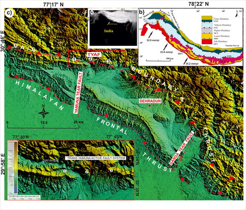
Figure 2. Geological map of the Trans-Yamuna area with faults, fluvial terraces and lithotectonic units. Terrace group assignments modeled after (Nossin 1971) and (Khan and Dubey 1981). Map modified after (Oatney et al. 2001).

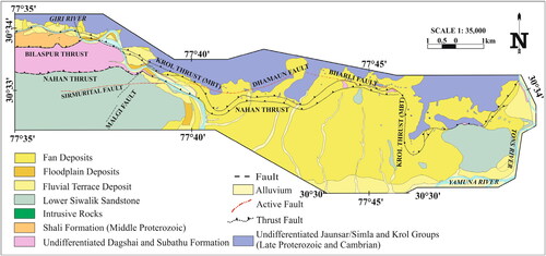
Broadly, the MBT separates the Lesser Himalayan Proterozoic rocks from the Early Tertiary sediments of the Sub Himalaya (Medlicott 1864). It brings the Pre-Tertiary rocks (Mandhali-Chandpur-Krol-Tal sequence; Damta Formation) over the Paleogene sedimentary sequence (Figure 2). The Mandhali formation, which can be found along the Giri River in the western part of the study area, is made up of pyritic slate with thin quartzite, chert, and limestone interbeds (Cp et al. 1976). Moreover, slate observed along the Tons River in the eastern part of the study area is also a part of the Mandhali formation (Sinvhal et al. 1973). In the western part of the Giri River, near Bhujon, the Krol Thrust brings rocks of the Jaunsar/Simla and Krol Groups over the older Precambrian rocks of the Shali Group. The Main Boundary Fault (MBF), locally known as the Bilaspur Thrust, brings the Paleogene rocks comprising the Subathu and Dagshai formations over the Lower and Middle Siwalik sequence (Virdi et al. 2006). Towards the east, we exclusively observe the Lower Siwalik rocks in between the Bilaspur thrust and the MBT. The Nahan Thrust brings the Lower Siwalik rocks, comprised of mudstones and siltstones, over the Upper Siwalik rocks (Figure 2). Its movement indicates a horizontal component of 0.902 cm/year in a 132 ^∘E direction and a strike slip component of 0.038 cm/year (Sinvhal et al. 1973). Although plate motion measurements in the Himachal Himalaya are very limited, a recent study by Mondal et al. (2022) reveals that the western part of NW Himalaya accumulates higher amount of strain rate than the eastern part of NW Himalaya. Low strain rate in the northwest Himalaya’s Himachal and Garhwal region is subject to strong crustal stress and is therefore expected to acquire more elastic energy than the Nepal and Kumaon region of the NW Himalaya. On the other hand, in NW Sub-Himalaya, shortening rates of 11 ± 5 mm/year across HFT were estimated over long term during the late Holocene (Powers et al. 1998; Wesnousky et al. 1999) for Dehradun in Garhwal Himalaya.

A number of cross and tear faults were observed crosscutting the Sub-Himalayan region in the N-S and NNE-SSW directions (Oatney et al. 2001). The Malgi Fault (Figure 2) is one such fault trending north-south, respectively which displaces the Nahan Thrust in the Trans-Yamuna region. As a result, structural deformation and landscape evolution in this region are mostly dominated by MBT and its splays, along with other faults and lineaments. It is worth noting that the Renuka lake, located in the NW part of the study area (refer Figure 1) is tectonically active and was formed as a result of block faulting along NNE-SSW trending lineaments (Virdi et al. 2006). Thus, the drainage in this region is observed to be structurally controlled as evidenced by its alignment along these structures or diversions due to the significant tectonic movement. The slopes pertaining to the Trans-Yamuna region are covered by Pleistocene to Holocene alluvial fan deposits, which are constituted of poorly sorted angular clasts in a light brown silt matrix derived from the pre-Tertiary sediments (Nossin 1971).

Furthermore, this region hosts the Trans-Yamuna Active Fault (TYAF), a left-stepping en echelon group of faults initially documented by Nossin (1971); Nakata (1972); Philip and Sah (1999). The TYAF is segmented into three parts, namely, Sirmurital, Dhamaun, and Bharli faults, as shown in (Figure 2), which is sub-parallel to and cuts across the MBT. Detailed satellite data analysis and fieldwork further reveal that these faults cut the Quaternary deposits of Late Holocene age (Oatney et al. 2001). The present study is focused on the Trans Yamuna region, with special emphasis on the TYAF and its activity.

3. Materials and methods

Sentinel-2 continues the Landsat and SPOT missions’ acquisition of providing high-resolution satellite data with a short revisit cycle (five days for Sentinel-2A and B) and has been perceived to be extremely significant for geological applications (Duputel et al. 2016). This product contains 13 spectral bands at various spatial resolutions, from 10 m–60 m (Van der Meer et al. 2014), which has been utilized for band-ratio technique in the present study. In addition, the False Colour Composite (FCC) of LANDSAT 7 ETM + satellite image was utilized for active fault mapping along with identification of geomorphic markers. The image was pan-sharpened with Cartosat-1 stereo-pair of 2.5 m spatial resolution. Details regarding the Cartosat-1 stereo-pairs is listed in Table 1.

Table 1. List of CartoSat-1 stereo pairs used for computing DEMs for the present study.

Date of acquisition	Stereo Pair Id	Path/Row
18-12-2011	163487671	526/257
29-12-2011	163487681	525/257
25-11-2014	163487691	524/257

DEMs collected from a number of public, commercial, and research agreement sources are listed in Supplementary Table 1. Four freely-available global DEM products were utilized for the study: (1) ASTER GDEM v2, (2) SRTM v3, (3) ALOS DEM (4) TanDEM-X, and (5) Carto-DEM prepared from commercially purchased stereopairs. For vertical accuracy assessment, TanDEM-X is considered as the reference DEM. Details pertaining to each dataset has been described in detail in the Supplementary file 1 (Section 1).

The methodology adopted is divided into three sections. Firstly, we present an analysis on the vertical accuracy of three freely available medium-resolution DEMs: ASTER GDEM2, SRTMv3.0 (hereafter called SRTM3), ALOS DEM, and a very high-resolution CARTO DEM (5 m) with respect to the highly accurate TanDEM-X for the study area. For co-registration, TanDEM-X is considered as the reference DEM due to its unprecedented horizontal and vertical (∼ 3.5 m absolute and < 2 m relative) accuracy (Rizzoli et al. 2017; Wessel 2018). Secondly, identification and mapping of active faults and associated geomorphic features were conducted utilizing Multispectral Sentinel 2 images and pan sharpened Landsat ETM + satellite image. Finally, the most appropriate digital elevation model (DEM) is used for morphotectonic analysis, which results in the presentation of an index of relative active tectonic activity (IRAT) for the TYAF region.

3.1. Active fault mapping using optical datasets

The present study utilized Google Earth Engine (GEE), a cloud-based platform, to analyze the Level-2A product of Sentinel-2, representing surface reflectance and ortho-rectified data. Although 13 spectral bands are available, the study considered the green (560 nm), vegetation red edge (VRE; 780 nm), near-infrared (NIR; 865 nm), and shortwave infrared (SWIR1 and SWIR2; 1610 nm and 2200 nm, respectively) bands. As the study focuses on geological features, a cloud-free composite imagery is generated from the image collection acquired during April and May, 2021 (summer season), to minimize the influence of vegetation in the analysis. To enhance the geological features of the study area, the current study used band ratio (BR) techniques, which involve dividing one spectral band by another, as proposed by Qureshi and Khan (2020). The first BR combination with SWIR2 upon VRE (as Red), SWIR2 upon Green (as Green) and SWIR2 upon SWR1 (as Blue) is used to differentiate younger wetter alluvial fans from older drier alluvial fans based on hydroxyl ion concentration (OH⁻). Whereas, the second BR combination with SWIR1 upon SWIR2 (as Red), SWIR2 upon VRE (as Green) and NIR upon SWR1 (as Blue), and the third BR combination with NIR upon SWIR1 (as Red), SWIR1 upon SWIR2 (as Green) and SWIR2 upon VRE (as Blue) were implemented. The second and third BR combinations enhance the different types of sedimentary rocks based on the clay content and surface texture. Figure 3 (a) (b) and (c) demonstrates a better overview of the above-mentioned band combinations. In addition, LANDSAT ETM + multispectral imagery was pansharpened with Cartosat-1 stereopair to identify geomorphic features and trace active faults in the region. PCI Geomatica 2015 software was utilized to process the images. The enhanced imagery after contrast stretching facilitated effortless identification and tracing of the fault scarps. Traditional visual interpretation techniques were used to confirm the results. Fieldwork was conducted prior to the onset of the monsoon season in the month of May, due to scanty rainfall and less vegetation during this time period. The field evidence further verified the geomorphic and tectonically active features in the field, as shown in Figure 4.

Figure 3. Sentinel-2B band ratios.

(a) 12/7-12/3-12/11 displayed as a RGB composite to discriminate lithology and structural elements. Inset 1 shows the enlarged view of that location with distinct view of the Giri river and associated landslides along its left banks. Inset 2 marks the numerous stream offsets observed across the MBT and active faults.

(b) 11/12-12/7-8/11; (c) 8/11-11/12-12/7 displayed as a RGB composite to discriminate lithology and structural elements. (d) Sentinel-2 true color composite (RGB: 432) is displayed to verify the same features as marked above. The inset 1 and 2 shows distinctly marked geomorphic features along with the active faults.

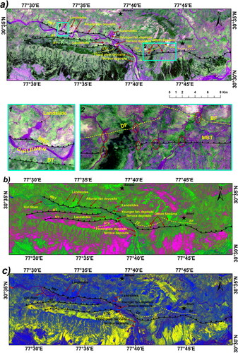
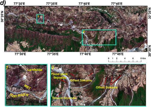
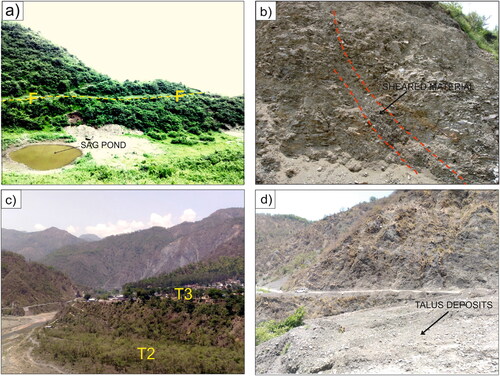
Figure 4. (a) Photograph showing the sag pond near the vicinity of the Bharli fault. Yellow line marks the Bharli fault. Location is marked as 1 in Figure 5. (b) Sheared Chandpur phyllite observed along the Bharli fault, at a road cut-section. Location is marked as 2 in Figure 5. (c) Photograph showing two levels of fluvial terraces (T2 and T3) in the Giri river flowing near Sataun region of NW Himalaya. Location is marked as 3 in Figure 5. (d) Landslide deposits observed along the left bank of the Giri river after crossing Sataun village. Location is marked as 4 in Figure 5.

3.2. DEM acquisition, processing and accuracy assessment

3.2.1. Stereo DEM generation

Stereo-DEM generation involves the reconstruction of surface topography with two or more overlapping optical images. The stereo-viewing capability of the Cartosat-1 satellite is exploited for three-dimensional point cloud determination, which further enables the generation of a DEM (Giribabu et al. 2013b). As reported in previous studies (Kocaman-Aksakal et al. 2008), the DEM generated from Cartosat-1 stereo imagery for undulating terrain contains a significant number of outliers due to the effect of shadow. Producing an accurate DEM requires post processing in the form of fill gap solutions, advanced filtering techniques, or manual editing, which are labour intensive and often error-prone (Toutin 2002; Reinartz et al. 2010). Keeping in mind the above listed issues, the present study is an attempt to derive high-quality terrain information for a highly undulating inaccessible Himalayan terrain falling in the MBT zone of NW Himalaya using an automated stereogrammetry software.

We used the open-source NASA Ames StereoPipeline (v.2.6.2) (Shean et al. 2016; Beyer et al. 2018; Beyer et al. 2019) to derive DEMs from two along-track CartoSat-1 stereo pairs as listed in Table 1. Prior to stereo correlation, the input RPC model parameters of each stereo pair were refined using ASP’s bundle adjust utility (Dehecq et al. 2020; Bhushan et al. 2021). This step minimises the triangulation error during subsequent stereo processing, resulting in more accurate and complete output point clouds. We employed ASP’s parallel_stereo algorithm individually on the three input stereo pairs and the corresponding refined RPC models to derive three sets of point clouds. The More Global Matching (MGM) correlation algorithm with a kernel size of 7 × 7 pixels, correlation tile size of 2048 pixels and the Bayes EM subpixel refinement algorithm were utilized, with all other correlation and triangulation parameters set to their default values. The output point clouds were gridded into DEMs at 5 m resolution with UTM 43 N (EPSG:32643) projection and heights relative to the WGS84 ellipsoid. We utilized point to plane Iterative Closest Point (ICP) routine (Pomerleau et al. 2013) implemented in ASP’s pc_align tool to co-register the output CartoSat-1 DEMs to publicly available 12.5 m ALOS DEM, further refining the absolute accuracy of our output DEMs.

3.2.2. Accuracy assessment

Prior to accuracy assessment, co-registration is mandatory, which basically determines and corrects the horizontal and vertical offsets between two DEMs after surface-to-surface matching. We aligned each candidate source DEM to TanDEM-X reference DEM using the (Nuth and Kääb 2011) method implemented in Shean et al. (2019). Thereafter, we analyzed the vertical accuracy of the candidate DEMs for our study by evaluating the residual median and normalized median absolute difference (NMAD) of elevation difference values with respect to the global 90 m TanDEM-X reference DEM (Rizzoli et al. 2017). The outline regarding the full co-registration workflow is listed in the dem_align.py script in the demcoreg package (Shean et al. 2019).

3.3. Geomorphic indices

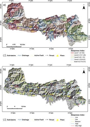
Geomorphic indices mirror the variations in the lithology and tectonic setting and one of the major objectives of the present study is to highlight the evidence of active tectonics and quantify it. The present study analyzes 41 sub-basins (714.6 km²), with their respective drainage either flowing parallel or across the strike of major faults, with the help of conventional geomorphic indices. The six indices include: Asymmetry factor (AF), Transverse Topographic Factor (TT), Hypsometric Integral (HI), Valley floor width ratio (Vf), Normalized Steepness Index (Ksn), and Stream Length Gradient Index (SL) (Bull and McFadden 2020; Keller and Pinter 1996; Kirby and Whipple 2001). Detailed information regarding each geomorphic indices is provided in Supplementary Table 2. To carry out the morphotectonic analysis we preferred very high resolution Cartosat DEM (5 m resolution) and utilized DEM processing tools in ArcGIS 10.5, CalHypso (Pérez-Peña et al. 2009), and TopoToolbox (Schwanghart and Kuhn 2010; Schwanghart and Scherler 2014). We analyzed different indices for each sub-basin and assigned them different tectonic classes based upon the range of values for individual respective geomorphic indices. Over the entire study region, these indices were summed, averaged, and classified into an index of relative active tectonics (IRAT) (El Hamdouni et al. 2008). We divided the geomorphic indices into 5 classes ranging from level 1 (Very high): 1.67-2.17, level 2 (High): 2.18-2.50, level 3 (Medium): 2.51-3.33, level 4 (Low): 3.34-3.67, and level 5 (very low): 3.68-4.20.

Table 2. Statistical vertical differences between the three global DEMs along with the high-resolution Cartosat DEM with respect to TanDEM-X expressed in terms of Median and NMAD in m.

	Before Alignment		After Alignment
Digital Elevation Model (DEM)	Median	NMAD	Median	NMAD
ALOS DEM	−2.00	5.93	0.00	5.93
ASTER DEM V3	1.02	9.06	0.07	8.04
SRTM V3	−2.24	6.74	−0.05	6.29
CARTO DEM	−2.27	9.35	0.04	6.15

4. Results

4.1. Active fault mapping and vertical error assessment of DEMs

The band ratio technique implemented on Sentinel-2 data enhanced the different lithological units, deflected streams, terrace deposits, alluvial fan deposits, and provided clarity on the different units developed in this tectonically active regime as observed in Figure 3 (a–d). Numerous active landslides are observed along both the banks of the Giri River along the major thrusts, which further corroborates the tectonic activity of the region (Figure 3 (a)–(c)). Deflected active streams along the major thrusts and faults validate the minor strike-slip component of the TYAF. Similarly, the development of different levels of fluvial terraces and alluvial fan deposits along the major streams, the formation of a sag pond near the Bharli fault, and the development of a pressure ridge explicitly verify the region’s tectonic activity. As observed in Figure 3 (a), the first BR combination clearly differentiates between the older and younger terrace deposits. Landslides are depicted in Figure 3(a) as dark purple and stands out against the green vegetated zones. The second and third BR combinations differentiate the units based on texture. Here, we can indubitably differentiate between the highly vegetated zone from the barren areas. Floodplain deposits can be easily differentiated from the terrace deposits in all the band combinations. The floodplain deposits appear light yellow in color whereas the terrace deposits appear light purple, as observed in BR 1 map (Figure 3(a)). The same is depicted as lighter and a darker shade of blue, respectively in BR 3 map (Figure 3(c)). Textural differences are more highlighted in BR 2 and 3. Finer sediments with a homogeneous texture appear in a lighter shade of blue in BR 3. Similarly, the light green colour on the BR 2 map represents loose silt and clay, which are mostly found in floodplain deposits along the river (Figure 3(b)). Vegetation is denoted by plum shade, which is observed mostly in the southern part of the study area. The True Color Composite (TCC) is provided to verify the results. The pan sharpened landsat ETM + image in (Figure 5) further demonstrates the presence of offset in streams across faults, the presence of a sag pond in the vicinity of the active fault, pressure ridge, and different levels of fluvial terraces, further confirming the trace of the active faults in the TYAF region of NW Himalayas. In addition, the major thrusts and faults are also explicitly observed in the satellite image.

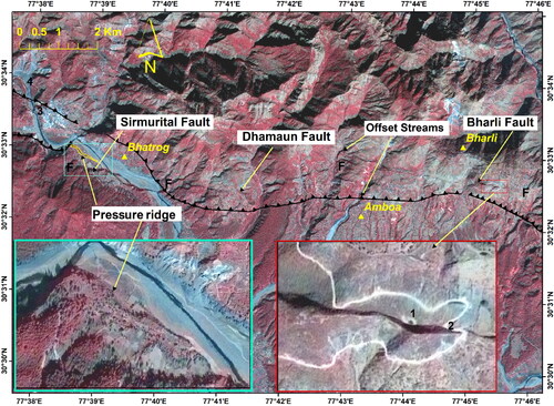
Figure 5. Landsat ETM + pan-sharpened image showing the three active faults. The oblique nature of the TYAF fault system can be easily demarcated in the satellite image. The numbers marked in black are the location of the field photographs displayed in figure 4. The inset (cyan rectangle) shows the enlarged view of a pressure ridge located at the vicinity of the Sirmurital fault. Similarly, the inset (red rectangle) is the enlarged view of the sag pond near the Bharli fault.

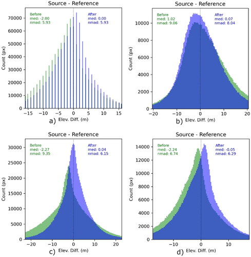
Furthermore, we tested the vertical accuracy of DEM data and observed that post geo-location correction, the vertical offsets between the input DEMs and the TanDEM-X reference DEM were minimised, as listed in Table 2. ALOS DEM and CartoSat-1 DEM demonstrated the lowest relative median bias and NMAD spread, followed by SRTM V3 and ASTER DEM V3 (Figure 6, Table 2). The histograms revealed a normal distribution, with deviation primarily in its symmetry.

Figure 6. It shows the final histograms of the elevation difference maps with respect to TanDEM-X DEM for (a) ALOS DEM, (b) ASTER DEM, (c) CARTO DEM, and (d) SRTM DEM. Median and NMAD values are shown before and after co-registration for each set of DEM.

4.2. Geomorphic indices and its spatial distribution

4.2.1. Asymmetry factor

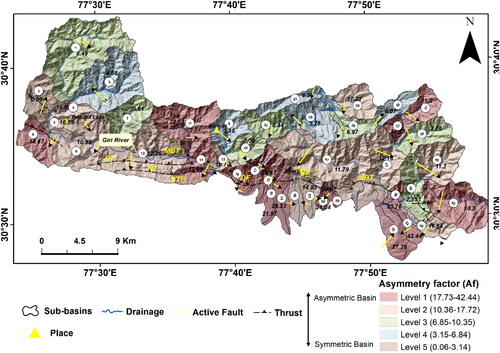
The present study expresses AF as an absolute value. It is the difference between the observed value of Af and 50. The value of AF substantially greater or smaller than 50 signifies the existence of active tectonics or lithological control (El Hamdouni et al. 2008; Mahmood and Gloaguen 2012). However, in tectonically active regions, the valley floor may move up or down relative to the surrounding slope or vice versa and may cause lateral river migration, eventually resulting in basin tilting. Figure 7 exhibits the thematic map of the AF values classified into five levels. 39% (i.e. 16 sub-basins) out of the total sub-basins fall under the level 1 category denoting highest asymmetry. However, 29% (12 sub-basins), 17% (7 sub-basins) and 12% (5 sub-basins) fall within the Level 2, Level 3 and Level 4 categories, respectively. The level 5 class consists of a single sub-basin with a negligible AF value of 0.06, which is considered to be stable.

Figure 7. Asymmetry factor map for the sub-basins showing widespread basin asymmetry factor and tilting direction related to relative active tectonics.

4.2.2. Transverse topography

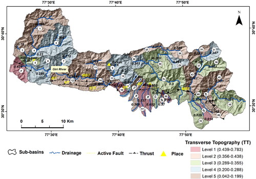
For each sub-basin, the TT values are calculated segment wise for the main stream at locations of considerable variability, and the mean value is computed to indicate the shifting of the main stream (Cox 1994). The TT values in the present study range from 0.042 to 0.685. As displayed in Figure 8, 14%, 17%, 21%, 24%, and 21% of the total basins fall under level 1, level 2, level 3, level 4 and level 5 categories, respectively. Almost 53% of the sub-basins indicate values of TT close to 1, exhibiting lateral migration of the trunk stream.

Figure 8. (a) Tranverse Topography (TT) map for the sub-basins showing four levels of active tectonic activity.

4.2.3. Hypsometric integral

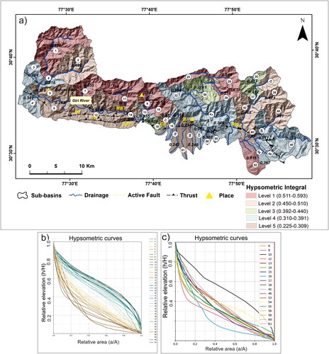
In tectonically active regions, the use of hypsometric curves can highlight the impact of tectonics on terrain (Delcaillau et al. 1998; Pérez-Peña et al. 2010). The values range from 0.22 to 0.56. However, sub-basins above MBT (sub-basins 7, 11, 09, and 10) demonstrate a higher HI value. As displayed in Figure 9a, 21% of the total basins fall under the Level 1 category. Similarly, 14%, 9%, 34%, and 19% fall under Level 2, Level 3, Level 4 and Level 5 categories, respectively. Figure 9(b) demonstrates the hypsometric curves for the entire study area.

Figure 9. (a) Hypsometric Integral map for the sub-basins showing five different classes from very high to low. (b) Graph showing the hypsometric curves for the entire study area, and (c) for the sub-basins associated with major thrusts and active faults.

4.2.4. Valley floor to valley height ratio

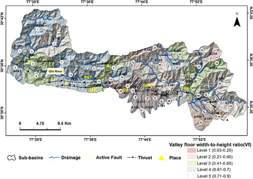
The value of Vf is calculated for valleys upstream from the mountain front at a particular distance (Silva et al. 2003). For the present study, the distance was set at 0.5 to 1 km upstream, depending on the size of the drainage basin. Vf values determined for 41 catchments range from 0.03 to 0.81 and demonstrate a scattered trend although maximum sub-basins formed V-shaped valleys. As displayed in Figure 10, 46% of the total basins fall under Level 1 and Level 2 category combined with very low Vf values.

Figure 10. Map showing different classes of Vf for the entire study area.

4.2.5. Stream length gradient index

Although high SL values on soft rocks suggest recent tectonic activity, anomalously low SL values can also imply tectonic activity when rivers and streams flow across strike-slip faults (Keller and Pinter 1996; Mahmood and Gloaguen 2012). The SL values in the present study range from 2.93 to 554. Almost 46% (i.e. 19 out of 41 sub-basins) from the present study display SL values above 100 as denoted in Figure 11(a). Basins 12 and 14, in spite of the presence of numerous thrusts and faults crossing them, exhibit low values of SL. This anomalous behavior has already been discussed previously and implies tectonic activity. For this reason, we have transposed basins 8 and 14 in the Level 1 category in order to avoid miscalculation in the final result. Furthermore, two cross profiles taken across the Giri River in sub-basins 1 and 14 display clear-cut evidence of the tectonically active features. Profile AA’ has been taken across Kandon ka Khala (refer Figure 11(a)). The knickpoints in the profile correspond to the Sirmurital Fault (STF), Bilaspur Thrust (BT), MBT, and the two levels of fluvial terraces (T1 and T2) (Figure 11(b)). Profile BB’ also depicts the lacustrine deposit in Sataun (ST), as well as the major thrusts and faults (Figure 11(c)).

Figure 11. (a) Map showing the Standardized SL-index values for all individual sub-basins. (b) and (c) are the cross profiles taken across the Sirmurital fault (STF). Location of the profiles (AA’ and BB’) is marked as yellow lines in Figure 11 (a). Figure (c) and (d) display the longitudinal Hack profile and SL index analysis of the Giri river flowing across sub-basin 15 and 17. The various structures encountered along the length of the rivers are shown on the river profiles.

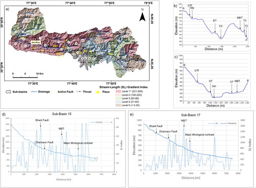
Profiles of sub-basins 15 and 17 as displayed in Figure 11(d) and (e) display prominent knickpoints with high SL values typical of a tectonic regime. Few basins exhibit very high SL values in the upstream reaches of the rivers due to high gradients and contrasting changes in lithology. However, most longitudinal profiles show a concave downward shape with prominent knickpoints, as displayed in Figure 11(d and e).

4.2.6. Steepness index

Generally, high and anomalous values of ksn have been associated with recent tectonic activity (Snyder et al. 2000; Pérez-Peña et al. 2010). For the present study, the ksn values range from 0.17 to 60.32 with considerable variations. Sub-basin 1 exhibited the highest steepness index due to its high gradient caused by lithological contrast as well as due to the presence of NE-SW trending lineaments above the MBT. Sub-basin 14 exhibits a very high value due to a change in its gradient as a consequence the presence of major thrusts and an anticline towards its south. The sub-basins in the vicinity of the active faults support the presence of both lithological and tectonic control. The lithology in this region consists of the Pre-tertiary sediments, the Tertiary Siwalik sediments, and the late Quaternary sediments. Figure 12(a) exhibits the average ksn values for each sub-basin. However, Figure 12(b) depicts a better picture of change in ksn values along the stream. As observed, in Figure 12(b) (note the white rectangle), a sharp increase in the values is observed at few locations as it crosses the active fault. Here, we correlate the change in values due to tectonic impulses post the generation of MBT.

Figure 12. (a) Map showing different classes of Steepness Index for the entire study area. (b) Map showing the Ksn variation across the major thrusts and faults in the TYAF region.

5. Discussion

5.1. Discussion on DEM accuracy

Preliminary identification and analysis of tectonic and geomorphic features in a drainage basin or fault zone has significantly progressed with the increasing availability of freely available satellite images (O'Callaghan and Mark 1984; Ozdemir and Bird 2009; Vincy et al. 2012). However, the resolution offered by the freely available DEMs is a constraint for catchment scale studies, which require detailed input data for the successful application of geomorphometry. In contrast to geomorphology, which relies on elevation derivatives, extensive study has been conducted on vertical accuracy with respect to glaciers, which primarily rely on absolute or relative height changes (Purinton and Bookhagen 2017). However, there has been a dearth of studies related to the vertical accuracy of DEMs for geomorphometry, especially the ones generated from stereo satellite images. It is a well-known fact that selecting a suitable DEM for morphotectonic studies in small river basins is still a conundrum. This is because the global estimate of root mean square error (RMSE) is the only information provided for every global DEM by the concerned agency, which varies as per different topography. For catchment scale studies, accuracy of the DEM at a specific location must be evaluated by the user.

The median and NMAD values are largest for the ASTER data post-alignment, indicating the importance of site-specific accuracy assessment for this dataset. Therefore, it is advisable to test the accuracy of the ASTER data prior to any analysis, especially in relation to morphotectonics. Similar results were documented globally by Suwandana et al. (2012); Zhang et al. (2019a); Liu et al. (2020), for the Himalayan region (Rawat et al. 2013; Mukherjee et al. 2013; Jain et al. 2018), and also for the present study. Purinton and Bookhagen (2017) observed relative inaccuracies in a variety of geomorphological terrains in the Central Andean Plate. They reported the largest vertical SD for ASTER, reassuring its inappropriateness for investigating morphological characteristics of a river or channel. Moreover, the orbital characteristics of the Terra satellite, according to Slater et al. (2011), may also have an influence on ASTER elevation data. Therefore, it is advisable to incorporate advanced smoothing and depression-filling algorithms. In general, SRTM is a preferbale dataset in terms of its good vertical accuracy in several studies conducted globally (De Vente et al. 2009; Thomas et al. 2014; Preety et al. 2022). Incorporating varied landcover classes into account, Hu et al. (2009) evaluated the accuracy of SRTM1, over China using a 1:50,000 scale TopoDEM and reported its preciseness in comparison to other global DEMs. These studies are in agreement with the observations of Kääb et al. (2005); Huggel et al. (2008) suggesting the efficiency of InSAR derived DEMs. However, in high relief areas, the SRTM DEM is subjected to foreshortening and shadowing, an inherent drawback of radar-based DEMs (Nelson et al. 2009). For the present study, the overall vertical accuracy of SRTM V3 data is preferably good as reported by its statistical values but must be verified prior to its usage for morphotectonic studies, especially for high-relief areas.

On the other hand, the ALOS DEM (12.5 m) outperformed all other DEMs in terms of its vertical accuracy. The pre and post alignment did not exhibit any changes in the NMAD values, and overall, the performance was best in terms of median and NMAD. Similar cases were observed in a few other studies conducted globally (Arabameri et al. 2019; Rabby et al. 2020; Ferreira and Cabral 2021).

Subsequently, the DEM generated by using the Cartosat-1 stereopairs seems to be an appropriate replacement for the ALOS DEM. As observed in Figure 6c, a significant reduction in error distribution is observed for the Cartosat-1 (5 m) DEM post alignment, with its median value nearly close to zero. However, for the present study, we require a DEM which has a combined advantage of good vertical accuracy and which identifies the minute details in the river channels. It is solely conceivable with a finer resolution DEM with good vertical accuracy. Cartosat-1 DEM exhibits explicit view of river channels cross cutting the faults in the TYAF region and its associated geomorphic features, in addition to being vertically accurate. In high relief areas where field survey is problematic, this study further emphasizes the development of a DEM without the use of GCPs. Despite the fact that the intrinsic inaccuracy in the rational function model accounts for the majority of the error in the absence of GCPs, procuring GCPs in a high-relief area is not always feasible (Aguilar et al. 2005; Wang et al. 2019). However, as a result of less vegetation in the current study area, the DEM errors were reduced. For morphotectonic research in the Himalayan region, the Cartosat-1 DEM, with its good vertical accuracy and very high resolution, can serve as a superior alternative to the ALOS DEM and SRTM DEMs, given the aforementioned benefits and drawbacks.

5.2. Geomorphometric validation and evaluation of IRAT

Substantial studies pertaining to relative tectonic activity based on geomorphic indices have been conducted globally but the sensitivity of DEMs was not taken into consideration, especially for catchment scale studies. As a result, the present study is an attempt to evaluate the tectonic activity in the TYAF zone of the Himalaya using a combination of multiple geomorphic indices by computing the averages of each parameter for a significant number of sub-basins and finally developing an index termed IRAT (Figure 13). The values of the index were classified into five classes to define the degree of active tectonics: Level 1 (Very high), Level 2 (High), Level 3 (Moderate), Level 4 (Low) and Level 5 (Very low). About 29% of the study area belongs to Level 1; 31% to Level 2; 21% to Level 3, 7% to Level 4, and 9% to Level 5.

Figure 13. Distribution of index of relative active tectonics (IRAT) in the Trans-Yamuna active fault region.

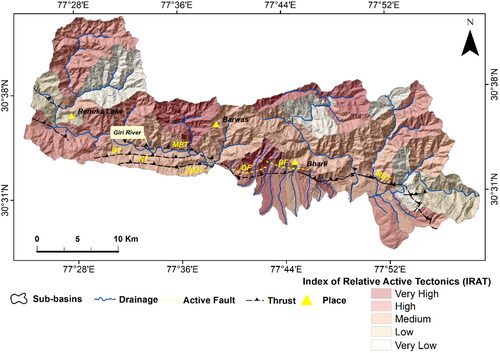
Our results are well corroborated with geomorphic features observed in satellite images in the form of fault scarp, terrace deposits and sag pond, with further verification in the field. As observed in Figure 13, the IRAT tends to be high along the TYAF zone and along the major thrusts pertaining to sub-basins 6, 8, and 16. The elongated nature of the sub-basins across the active faults further indicates a strong structural control. The AF values reveal that almost all the sub-basins are asymmetrically developed, except for six sub-basins which exhibit stable behavior, exhibiting minute lateral shifting of drainage. The sub-basins of the Giri river crossing the MBT exhibit high asymmetric values and are tilted towards the SW. The AF values of the sub-basins crossing the active faults indicate major tilt direction towards the east as displayed in Figure 7. In sub-basin 55 and 58, the influence of the active faults diminishes and, hence, the vertical uplift of the MBT plays a major role in this domain. Furthermore, sub-basin no. 52 and 54 exhibit high asymmetry factor values due to lithological contrast and a sudden change in gradient which influences the basin tilt. Similar is the case with sub-basin no’s 26, 30 and 31 located in the Pre-tertiary formation. Therefore, north of the MBT, no defined value of AF is observed. A synergistic use of both AF and TT values indicates the preferential direction of stream movement, thereby confirming lateral migration and asymmetric development of basins (Goswami and Kshetrimayum 2020). The TT values of sub-basins in the vicinity of the MBT crossing the Giri River are highly asymmetric, attributed to the presence of major thrusts in this region. To the north of the MBT, however, the TT values do not indicate a clear preferred direction and may be influenced by lithological variations and localized activity. We notice moderate and low values of HI for the sub-basins associated with the major thrusts and active faults (Figure 9c). This is due to the complex nature of compressional tectonics and the strike slip nature of faults at this junction. Furthermore, according to Mahmood and Gloaguen (2012) in their study on the Hindu-Kush Himalaya, if part of the HI curve is convex in the lower region despite low values, it could indicate fault uplift or recent thrusting. Figure 9(c) depicts a similar scenario observed in our analysis. High values of HI are observed in sub-basins 7, 9, 10, and 11 as shown in Figure 9(a). Furthermore, as shown in Figure 9(c), sub-basins 53, 55, and 58 demonstrate complex curves with a convex shape at the lower end. The effect of active faults dies out in this zone, with the sole influence of MBT. However, in case of Vf the possible reasons for very low values in the vicinity of the active faults is due to intense erosion in this zone and the presence of Quaternary sediments. However, the basins in the vicinity of the MBT are influenced by landslides and active alluvial plains, which transform them into wide river valleys with moderate values of Vf. Moreover, high SL indices above the MBT in the left bank of the Giri River can be broadly attributed to change in gradient due to uplift along with sharp change in lithology between the Pre-Tertiaries and the Tertiaries and also due to the presence of NW-SE trending lineaments as displayed in Figure 11(a).

Evidence of drainage offsets at a few locations along the TYAF suggests a minor strike-slip component along with normal faulting. Prominent knickpoints observed in the longitudinal profiles complemented with high SL values justify the inferences. The existence of high values of the SL index north of the MBT in the pre-Tertiary rocks highlights the domination of the tectonic processes over erosional processes. All the sub-basins underlying the Giri river demonstrate significant evidence of active tectonics. However, sub-basin 12, although traversed by several active tectonic features in the form of major thrusts and uplifted alluvial terraces, exhibits a moderate IRAT value due to very low values for the parameters TT and HI (Level 5). Overall, the quantitative parameters pertaining to IRAT suggest upliftment due to active tectonics in this part of the terrain.

Preliminary studies by Philip and Sah (1999) had observed tributary channels joining at right angles to the main stream (i.e. Giri River) indicating high terrain gradient, distinct elevation levels for alluvial fans on the left bank of the Giri river, suggesting the upliftment towards the north. Similar geomorphic features were observed by Valdiya et al. (1992); Philip et al. (2017); Luirei et al. (2021) in different segments of the Himalaya pertaining to the MBT. Furthermore, normal faulting with a minor strike-slip component as reported in the TYAF, as well as the formation of a sag pond, are classic examples of tectonically active terrain. Our study substantiates that elastic strain release within the hanging wall is not limited to the front, but is diffused over a larger region above the decollement, with 10-15% of the total Quaternary shortening accommodated within the interiors of the Himalaya in the hanging wall of the MBT or other structures (Deeken et al. 2011; Thiede et al. 2017; Dey et al. 2020). The Logar Fault in the northwestern Kumaon Sub Himalaya has vertically dismembered the Quaternary alluvial fan and subsequent paleoseismic investigations suggest multiple faulting events along this fault (Philip et al. 2017). Normal faulting north of the MBT is also observed in the Kosi river valley (Luirei et al. 2021), Nepal and Darjeeling foothills (Heim 1938; Hagen 1956), Kumaon Himalaya (Valdiya et al. 1992), and Arunachal Himalaya (Luirei et al. 2021).

6. Conclusions

This study is a first attempt towards quantifying the relative tectonic activity in the Trans-Yamuna region of the NW Himalaya using a very high-resolution DEM of 5 m derived from Cartosat-1 satellite data. The region falls within the central Himalayan seismic gap, which is 700 km long and lies between the 1905 Kangra earthquake and the 1934 Nepal-Bihar earthquake events (Khattri, 1987). Therefore, the identification and mapping of active faults along with a complex geological setup aids towards seismic hazard assessment towards the highly populated townships located in this region. We identified several Quaternary landforms in the form of uplifted alluvial fans, offset streams, pressure ridges, and sag ponds, in the high-resolution satellite image (Figures 3 and 5). They represent vulnerable zones that have accumulated strain from major earthquakes in the late Quaternary and Holocene and could rupture in the future. Therefore, to assess the spatial distribution of late Quaternary deformation, we established an index of relative tectonic activity for the region. On the basis of this study, the following conclusions have been drawn:

1. The results generate insights into differential tectonic uplift patterns in the TYAF region, with substantial vertical uplifting north of the MBT, being attributed to active tectonics.

2. Based on the vertical accuracy assessment of DEMs we infer that Cartosat-1 DEM due to its good vertical accuracy and high resolution can be the preferred DEM for geomorphic analysis in the Himalayan region.

3. The study further substantiates the fact that strain release is distributed over a broader area further north of the MBT.

In addition, our study adds a new dimension to morphotectonic studies by a combined analysis of geomorphic studies with field verification along with special emphasis on the input parameters, i.e. vertical accuracy of DEMs. It emphasized on the importance of assessing the vertical accuracy of DEMs for morphotectonic analysis in the Himalayan region and strongly suggests researchers to perform a site-specific assessment of DEMs before undertaking any morphotectonic studies, especially on a catchment scale for unbiased analysis. The current study highlights the need for further studies to constrain the rates of vertical deformation in the TYAF region of the NW Himalaya.   

Author credit statement

G.Philip: Conceptualization, Funding acquisition, Investigation, Project administration, Supervision and finalization of draft. S.Ghosh: Conceptualization, Methodology, Software, Formal analysis, Investigation, Data curation, Writing - Original draft. A. Prasad: Partial writing, Supervision and finalization of draft. T.H Syed: Conceptualization, Supervision and finalization of draft. S. Mohanty: Initial discussion and finalization of draft.

Acknowledgements

The authors are grateful to the Chairman, ISRO for sponsoring the study under the collaborative program between WIHG and ISRO-IIRS. We are also grateful to the Directors of the Indian Institute of Remote Sensing and the Wadia Institute of Himalayan Geology at Dehradun for their continuous support and encouragement to carry out the study. We thank Shashank Bhushan from the University of Washington for DEM analysis and technical assistance. The authors would like to thank Google (LLC) for Google Earth and Google Earth Engine Cloud Platform. We extend our heartfelt gratitude to Late Dr. Prashant K. Champati ray who left us forever during the second peak of Covid-19 pandemic and was an integral part of this project. The authors also extend their thanks to the anonymous reviewers for their thorough reviews and valuable suggestions, which were of great help in improving the manuscript.

Data availability statement

All the data-sets will be available from the authors upon reasonable request.

Disclosure statement

No potential conflict of interest was reported by the authors.

Additional information

Funding

This work was supported by Indian Space Research Organisation (ISRO) under the Earth Observation Application Mission (EOAM) project scheme.

References

- Ader T, Avouac JP, Liu-Zeng J, Lyon-Caen H, Bollinger L, Galetzka J, Genrich J, Thomas M, Chanard K, Sapkota SN, et al. 2012. Convergence rate across the Nepal Himalaya and interseismic coupling on the main himalayan thrust: implications for seismic hazard. J Geophys Res. 117(B4):n/a–n/a.
- Aguilar FJ, Agüera F, Aguilar MA, Carvajal F. 2005. Effects of terrain morphology, sampling density, and interpolation methods on grid dem accuracy. Photogramm Eng Remote Sensing. 71(7):805–816.
- Ahmed N, Mahtab A, Agrawal R, Jayaprasad P, Pathan SK, Singh DK, Singh, AK, Ajai. 2007. Extraction and validation of cartosat-1 DEM. J Indian Soc Remote Sens. 35(2):121–127.,
- Arabameri A, Pradhan B, Rezaei K, Lee CW. 2019. Assessment of landslide susceptibility using statistical-and artificial intelligence-based fr–rf integrated model and multiresolution DEMs. Remote Sens. 11(9):999.
- Arora S, Malik JN, Sahoo S. 2019. Paleoseismic evidence of a major earthquake event (s) along the hinterland faults: Pinjore garden fault (PGF) and Jhajra fault (JF) in Northwest Himalaya. India. Tectonophysics. 757:108–122.
- Banerjee P, Bürgmann R. 2002. Convergence across the northwest Himalaya from GPS measurement. Geophys Res Lett. 29:13.
- Bettinelli P, Avouac JP, Flouzat M, Jouanne F, Bollinger L, Willis P, Chitrakar GR. 2006. Plate motion of India and interseismic strain in the nepal himalaya from gps and doris measurements. J Geodesy. 80(8–11):567–589.
- Beyer R, Alexandrov O, McMichael S. 2019. Neogeographytoolkit/stereopipeline: Asp 2.6. 2 (version v2. 6.2). zenodo. https://doi.org/10.5281/zenodo.3247734
- Beyer RA, Alexandrov O, McMichael S. 2018. The AMES stereo pipeline: Nasa’s open source software for deriving and processing terrain data. Earth Space Sci. 5(9):537–548.
- Bhushan S, Shean D, Alexandrov O, Henderson S. 2021. Automated digital elevation model (DEM) generation from very-high-resolution planet skysat triplet stereo and video imagery. ISPRS J Photogramm Remote Sens. 173:151–165.
- Bishop P. 2007. Long-term landscape evolution: linking tectonics and surface processes. Earth Surf Process Landforms. 32(3):329–365.
- Bollinger L, Sapkota SN, Tapponnier P, Klinger Y, Rizza M, Van Der Woerd J, Tiwari D, Pandey R, Bitri A, Bes de Berc S. 2014. Estimating the return times of great himalayan earthquakes in Eastern Nepal: evidence from the Patu and Bardibas strands of the main frontal thrust. J Geophys Res Solid Earth. 119(9):7123–7163.
- Braun A. 2021. Retrieval of digital elevation models from sentinel-1 radar data–open applications, techniques, and limitations. Open Geosciences. 13(1):532–569.
- Buczek K, Górnik M. 2020. Evaluation of tectonic activity using morphometric indices: case study of the tatra mts.(western carpathians, poland). Environ Earth Sci. 79(8):1–13.
- Bull WB, McFadden LD. 2020. Tectonic geomorphology north and south of the Garlock Fault, California. Geomorphology in arid regions. Routledge; p. 115–138.
- Burbank DW, Anderson RS. 2011. Tectonic geomorphology. John Wiley & Sons, USA.
- Cox RT. 1994. Analysis of drainage-basin symmetry as a rapid technique to identify areas of possible quaternary tilt-block tectonics: an example from the Mississippi embayment. Geol Soc America Bull. 106(5):571–581.
- De Vente J, Poesen J, Govers G, Boix-Fayos C. 2009. The implications of data selection for regional erosion and sediment yield modelling. Earth Surf Process Landforms. 34(15):1994–2007.
- Deeken A, Thiede R, Sobel E, Hourigan J, Strecker M. 2011. Exhumational variability within the Himalaya of Northwest India. Earth Planet Sci Lett. 305(1-2):103–114.
- Dehbozorgi M, Pourkermani M, Arian M, Matkan A, Motamedi H, Hosseiniasl A. 2010. Quantitative analysis of relative tectonic activity in the Sarvestan Area, Central Zagros, Iran. Geomorphology. 121(3–4):329–341.
- Dehecq A, Gardner AS, Alexandrov O, McMichael S, Hugonnet R, Shean D, Marty M. 2020. Automated processing of declassified kh-9 hexagon satellite images for global elevation change analysis since the 1970s. Front Earth Sci. 8:566802.
- Delcaillau B, Deffontaines B, Floissac L, Angelier J, Deramond J, Souquet P, Chu HT, Lee J. 1998. Morphotectonic evidence from lateral propagation of an active frontal fold; pakuashan anticline, foothills of Taiwan. Geomorphology. 24(4):263–290.
- Dey S, Thiede R, Biswas A, Chakravarti P, Jain V, Dey S. 2020. Structural variations in basal decollement and internal deformation of the lesser Himalayan duplex trigger landscape morphology in NW Himalayan interiors. Earth Surf Dyn Discuss. 2020:1–40.
- Divyadarshini A, Singh V. 2017. Identifying active structures in the Chitwan Dun, Central Nepal, using longitudinal river profiles and sl index analysis. Quat Int. 462:176–193.
- Duputel Z, Vergne J, Rivera L, Wittlinger G, Farra V, Hetényi G. 2016. The 2015 Gorkha earthquake: a large event illuminating the main Himalayan thrust fault. Geophys Res Lett. 43(6):2517–2525.
- El Hamdouni R, Irigaray C, Fernández T, Chacón J, Keller E. 2008. Assessment of relative active tectonics, southwest border of the Sierra Nevada (Southern Spain). Geomorphology. 96(1–2):150–173.
- England P, Molnar P. 1990. Surface uplift, uplift of rocks, and exhumation of rocks. Geol. 18(12):1173–1177.
- Ferreira ZA, Cabral P. 2021. Vertical accuracy assessment of alos palsar, gmted2010, srtm and topodata digital elevation models. In: Proceedings of the 7th International Conference on Geographical Information Systems Theory, Applications and Management (GISTAM 2021). SciTePress-Science and Technology Publications; p. 116–124.
- Finley T, Salomon G, Nissen E, Stephen R, Cassidy J, Menounos B. 2021. Preliminary results and structural interpretations from drone lidar surveys over the eastern Denali fault. Yukon. Yukon Explor Geol. 2021:83–106.
- Fisher PF, Tate NJ. 2006. Causes and consequences of error in digital elevation models. Prog Phys Geogr. 30(4):467–489.
- Florinsky IV. 1998. Accuracy of local topographic variables derived from digital elevation models. Int J Geogr Information Sci. 12(1):47–62.
- Gansser A. 1964. Geology of the Himalayas. London: Wiley.
- Gao M, Hugenholtz CH, Fox TA, Kucharczyk M, Barchyn TE, Nesbit PR. 2021. Weather constraints on global drone flyability. Sci Rep. 11(1):1–13.
- Gao M, Zeilinger G, Xu X, Wang Q, Hao M. 2013. DEM and GIS analysis of geomorphic indices for evaluating recent uplift of the northeastern margin of the Tibetan Plateau, China. Geomorphology. 190:61–72.
- Gautam PK, Gahalaut V, Prajapati SK, Kumar N, Yadav RK, Rana N, Dabral CP. 2017. Continuous gps measurements of crustal deformation in Garhwal-Kumaun Himalaya. Quat Int. 462:124–129.
- Giribabu D, Kumar P, Mathew J, Sharma K, Murthy YK. 2013a. DEM generation using cartosat-1 stereo data: issues and complexities in Himalayan terrain. Eur J Remote Sens. 46(1):431–443.
- Giribabu D, Rao SS, Murthy YK. 2013b. Improving cartosat-1 DEM accuracy using synthetic stereo pair and triplet. ISPRS J Photogramm Remote Sens. 77:31–43.
- Goswami PK, Kshetrimayum AS. 2020. Pattern of active tectonic deformation across the Churachandpur-Mao thrust zone of Manipur hills, Indo-Myanmar range, NE India: inferences from geomorphic features and indices. Quat Int. 553:144–158.
- Guo P, Han Z, Dong S, Gao F, Li J. 2021. New constraints on slip behavior of the Jianshui strike-slip fault from faulted stream channel risers and airborne lidar data, SE Tibetan plateau, China. Remote Sensing. 13(10):2019.
- Hack JT. 1973. Stream-profile analysis and stream-gradient index. J Res US Geol Survey. 1(4):421–429.
- Hagen T. 1956. Über eine überschiebung der tertiären siwaliks über das rezente ganges alluvium in ostnepal. Geogr Helv. 11(1):217–219.
- Hassen MB, Deffontaines B, Turki MM. 2014. Recent tectonic activity of the gafsa fault through morphometric analysis: Southern Atlas of Tunisia. Quat Int. 338:99–112.
- Heim A. 1938. The Himalayan border compared with the alps. Rec Geol Surv India. 72(Part 4):413–421.
- Hetényi G, Le Roux-Mallouf R, Berthet T, Cattin R, Cauzzi C, Phuntsho K, Grolimund R. 2016. Joint approach combining damage and paleoseismology observations constrains the 1714 AD Bhutan earthquake at magnitude 8 ± 0.5. Geophys Res Lett. 43(20):10,695–10,702.
- Holbrook J, Schumm SA. 1999. Geomorphic and sedimentary response of rivers to tectonic deformation: a brief review and critique of a tool for recognizing subtle epeirogenic deformation in modern and ancient settings. Tectonophysics. 305(1–3):287–306.
- Hu P, Liu X, Hu H. 2009. Accuracy assessment of digital elevation models based on approximation theory. Photogramm Eng Remote Sensing. 75(1):49–56.
- Huggel C, Schneider D, Miranda PJ, Granados HD, Kääb A. 2008. Evaluation of aster and SRTM DEM data for Lahar modeling: a case study on Lahars from popocatépetl volcano, Mexico. J Volcanol Geotherm Res. 170(1–2):99–110.
- Jade S, Mukul M, Gaur V, Kumar K, Shrungeshwar T, Satyal G, Dumka RK, Jagannathan S, Ananda M, Kumar PD, et al. 2014. Contemporary deformation in the Kashmir–Himachal, Garhwal and Kumaon Himalaya: significant insights from 1995–2008 GPS time series. J Geod. 88(6):539–557.
- Jain AO, Thaker T, Chaurasia A, Patel P, Singh AK. 2018. Vertical accuracy evaluation of SRTM-gl1, GDEM-v2, aw3d30 and cartodem-v3. 1 of 30-m resolution with dual frequency GNSS for lower Tapi basin India. Geocarto Int. 33(11):1237–1256.
- Jayangondaperumal R, Daniels RL, Niemi TM. 2017. A paleoseismic age model for large-magnitude earthquakes on fault segments of the himalayan frontal thrust in the central seismic gap of Northern India. Quat Int. 462:130–137.
- Kääb A, Huggel C, Fischer L, Guex S, Paul F, Roer I, Salzmann N, Schlaefli S, Schmutz K, Schneider D, et al. 2005. Remote sensing of glacier-and permafrost-related hazards in high mountains: an overview. Nat Hazards Earth Syst Sci. 5(4):527–554.
- Karabulut MS, Özdemir H. 2019. Comparison of basin morphometry analyses derived from different DEMs on two drainage basins in Turkey. Environ Earth Sci. 78(18):574.
- Keller E, Pinter N. 1996. Active tectonics prentice hall. Upper Saddle River, NJ; p. 338.
- Khalifa A, Bashir B, Alsalman A, Öğretmen N. 2021. Morpho-tectonic assessment of the Abu-Dabbab area, Eastern Desert, Egypt: insights from remote sensing and geospatial analysis. IJGI. 10(11):784.
- Khalifa A, Çakir Z, Owen, L, Kaya Ş. 2019. Evaluation of the relative tectonic activity of the ad Iyaman fault within the Arabian-anatolian plate boundary (Eastern Turkey). Geol Acta. 17(1):1–17.
- Khan A, Dubey U. 1981. Study of river terrace in Ganga river complex in Garhwa L Himalaya. Man Environ ISPQUS. 4:6–12.
- Khattri KN. 1987. Great earthquakes, seismicity gaps and potential for earthquake disaster along the Himalaya plate boundary. Tectonophysics. 138(1):79–92.
- Kirby E, Whipple K. 2001. Quantifying differential rock-uplift rates via stream profile analysis. Geol. 29(5):415–418.
- Kirby E, Whipple KX. 2012. Expression of active tectonics in erosional landscapes. J Struct Geol. 44:54–75.
- Kocaman-Aksakal S, Wolff K, Gruen A, Baltsavias E. 2008. Geometric validation of cartosat-1 imagery. Int Archiv Photogrammetr Remote Sens Spatial Inform Sci. 37(B1):1363–1368.
- Kothyari GC, Joshi N, Thakur M, Taloor AK, Pathak V. 2021. Reanalyzing the geomorphic developments along tectonically active soan thrust, NW Himalaya, India. Quaternary Sci Adv. 3:100017.
- Kumahara Y, Jayangondaperumal R. 2013. Paleoseismic evidence of a surface rupture along the Northwestern Himalayan Frontal Thrust (hft). Geomorphology. 180–181:47–56.
- Kumar A, Negi H, Kumar K, Shekhar C. 2020. Accuracy validation and bias assessment for various multi-sensor open-source DEMs in part of the Karakoram region. Remote Sens Lett. 11(10):893–902.
- Kumar S, Wesnousky SG, Jayangondaperumal R, Nakata T, Kumahara Y, Singh V. 2010. Paleoseismological evidence of surface faulting along the Northeastern Himalayan Front, India: timing, size, and spatial extent of great earthquakes. J Geophys Res. 101(6):3060–3064.
- Kumar S, Wesnousky SG, Rockwell TK, Ragona D, Thakur VC, Seitz GG. 2001. Earthquake recurrence and rupture dynamics of Himalayan Frontal Thrust, India. Science. 294(5550):2328–2331.
- Kundu B, Yadav RK, Bali BS, Chowdhury S, Gahalaut V. 2014. Oblique convergence and slip partitioning in the NW Himalaya: implications from GPS measurements. Tectonics. 33(10):2013–2024.
- Langridge RM, Howarth JD, Cox SC, Palmer JG, Sutherland R. 2018. Frontal fault location and most recent earthquake timing for the alpine fault at Whataroa, Westland, New Zealand. New Zealand J Geol Geophys. 61(3):329–340.
- Lavé J, Yule D, Sapkota S, Basant K, Madden C, Attal M, Pandey R. 2005. Evidence for a great medieval earthquake (˜ 1100 AD) in the Central Himalayas. Science. 307(5713):1302–1305.
- Le Roux-Mallouf R, Ferry M, Ritz JF, Berthet T, Cattin R, Drukpa D. 2016. First paleoseismic evidence for great surface-rupturing earthquakes in the bhutan himalayas. J Geophys Res Solid Earth. 121(10):7271–7283.
- Liang Z, Wei Z, Sun W, Zhuang Q. 2021. Surface slip distribution and earthquake rupture model of the Fuyun Fault, China, based on high-resolution topographic data. Lithosphere. 2021(Special 2):7913554.
- Liu Z, Zhu J, Fu H, Zhou C, Zuo T. 2020. Evaluation of the vertical accuracy of open global DEMs over steep terrain regions using icesat data: a case study over Hunan Province, China. Sensors. 20(17):4865.
- López C. 1997. Locating some types of random errors in digital terrain models. Int J Geograph Inform Sci. 11(7):677–698.
- Luirei K, Ch Kothyari G, Mehta M. 2022. Active tectonics in the main boundary thrust zone, Garhwal Himalaya, as evident from palaeoseismic signatures, morphotectonic features and PSI base ground deformation. Geol J. 1–14. https://doi.org/10.1002/gj.4586
- Luirei K, Lokho K, Longkumer L, Kothyari GC, Rai R, Rawat IS, Nakhro D. 2021. Morphotectonic evolution of the quaternary landforms in the Yangui river basin in the Indo-Myanmar range. J Asian Earth Sci. 218:104877.
- Lyon-Caen H, Molnar P. 1985. Gravity anomalies, flexure of the Indian plate, and the structure, support and evolution of the Himalaya and Ganga basin. Tectonics. 4(6):513–538.
- Mahmood S, Gloaguen R. 2012. Appraisal of active tectonics in Hindu Kush: insights from DEM derived geomorphic indices and drainage analysis. Geosci Front. 3(4):407–428.
- Malik JN, Sahoo AK, Shah AA, Shinde DP, Juyal N, Singhvi AK. 2010. Paleoseismic evidence from trench investigation along hajipur fault, himalayan frontal thrust, NW Himalaya: implications of the faulting pattern on landscape evolution and seismic hazard. J Struct Geol. 32(3):350–361.
- Medlicott HB. 1864. On the geological structure and relations of the Himalayan ranges, between the rivers ganges and Ravee. Mem Geol Surv India. 3:102.
- Mondal SK, Yadav RK, Bansal AK, Catherine JK, Gahalaut VK. 2022. Geodetic strain rate, slip deficit and seismicity analysis in Central Seismic Gap of the Himalayan arc. Himalayan Geol. 43(1B):140–150.
- Mukhamediev RI, Symagulov A, Kuchin Y, Zaitseva E, Bekbotayeva A, Yakunin K, Assanov I, Levashenko V, Popova Y, Akzhalova A, et al. 2021. Review of some applications of unmanned aerial vehicles technology in the resource-rich country. Appl Sci. 11(21):10171.
- Mukherjee S, Joshi PK, Mukherjee S, Ghosh A, Garg R, Mukhopadhyay A. 2013. Evaluation of vertical accuracy of open source digital elevation model (dem). Int J Appl Earth Obs Geoinf. 21:205–217.
- Nakata T. 1972. Geomorphic history and crustal movement of the foot-hills of the Himalayas. Science Report Tohoku Univ 7th Series (Geography). 22:39–177.
- Nakata T. 1989. Active faults of the Himalaya of India and Nepal. In: Tectonics of the Western Himalayas. vol. 232. Geological Society of America. 232(1): 243–264.
- Nelson A, Reuter H, Gessler P. 2009. Dem production methods and sources. Developments in Soil Sci. 33:65–85.
- Nossin J. 1971. Outline of the geomorphology of the Doon valley, Northern UP, India. Zeitschrift Geomorphology NF. 12:18–50.
- Nuth C, Kääb A. 2011. Co-registration and bias corrections of satellite elevation data sets for quantifying glacier thickness change. The Cryosphere. 5(1):271–290.
- Oatney E, Virdi N, Yeats R. 2001. Contribution of trans-Yamuna active fault system towards hanging wall strain release above the décollement, Himalayan Foothills of Northwest India. Himalayan Geol. 22(2):9–27.
- O'Callaghan JF, Mark DM. 1984. The extraction of drainage networks from digital elevation data. Computer Vision, Graphics, and Image Processing. 28(3):323–344.
- Ozdemir H, Bird D. 2009. Evaluation of morphometric parameters of drainage networks derived from topographic maps and dem in point of floods. Environ Geol. 56(7):1405–1415.
- Pandey M, Tandukar R, Avouac J, Lave J, Massot J. 1995. Interseismic strain accumulation on the Himalayan crustal ramp (Nepal). Geophys Res Lett. 22(7):751–754.
- Pandey P, Manickam S, Bhattacharya A, Ramanathan A, Singh G, Venkataraman G. 2017. Qualitative and quantitative assessment of Tandem-X DEM over Western Himalayan glaciated terrain. Geocarto Int. 32(4):442–454.
- Pandey P, Venkataraman G. 2012. Generation and evaluation of cartosat- 1 DEM for Chhota Shigri Glacier, Himalaya. Int J Geomatics and Geosci. 2(3):704–711.
- Pérez-Peña JV, Azañón JM, Azor A. 2009. Calhypso: An arcgis extension to calculate hypsometric curves and their statistical moments. applications to drainage basin analysis in SE Spain. Comput Geosci. 35(6):1214–1223.
- Pérez-Peña JV, Azor A, Azañón JM, Keller EA. 2010. Active tectonics in the Sierra Nevada (Betic Cordillera, SE Spain): insights from geomorphic indexes and drainage pattern analysis. Geomorphology. 119(1–2):74–87.
- Philip G, Bhakuni S, Suresh N. 2012. Late pleistocene and holocene large magnitude earthquakes along Himalayan frontal thrust in the central seismic gap in NW Himalaya, Kala Amb, India. Tectonophysics. 580:162–177.
- Philip G, Sah MP. 1999. Geomorphic signatures of active tectonics in the trans-yamuna segment of the Western Doon Valley, Northwest Himalaya, India. Int J Appl Earth Obs Geoinf. 1(1):54–63.
- Philip G, Suresh NP, Jayangondaperumal R. 2017. Late pleistocene-holocene strain release by normal faulting along the main boundary thrust at logar in the Northwestern Kumaon Sub Himalaya, India. Quat Int. 462:50–64.
- Pinter A, Keller, EA. 2002. Active tectonics: earthquakes, uplift, and landscape. Prentice Hall, 362p.
- Pomerleau F, Colas F, Siegwart R, Magnenat S. 2013. Comparing ICP variants on real-world data sets. Auton Robot. 34(3):133–148.
- Powers PM, Lillie RJ, Yeats RS. 1998. Structure and shortening of the Kangra and Dehra Dun reentrants, sub-Himalaya, India. Geol Soc Am Bull. 110(8):1010–1027.
- Preety K, Prasad AK, Varma AK, El-Askary H. 2022. Accuracy assessment, comparative performance, and enhancement of public domain digital elevation models (aster 30 m, srtm 30 m, cartosat 30 m, srtm 90 m, merit 90 m, and tandem-x 90 m) using DGPS. Remote Sens. 14(6):1334.
- Purinton B, Bookhagen B. 2017. Validation of digital elevation models (DEMs) and comparison of geomorphic metrics on the Southern Central Andean Plateau. Earth Surf Dynam. 5(2):211–237.
- Qureshi KA, Khan SD. 2020. Active tectonics of the frontal Himalayas: An example from the manzai ranges in the recess setting, Western Pakistan. Remote Sens. 12(20):3362.
- Rabby YW, Ishtiaque A, Rahman M. 2020. Evaluating the effects of digital elevation models in landslide susceptibility mapping in Rangamati District, Bangladesh. Remote Sens. 12(17):2718.
- Rastogi G, Agrawal, R, Ajai. 2015. Bias corrections of cartodem using icesat-glas data in hilly regions. GIScience & Remote Sens. 52(5):571–585.
- Rawat KS, Mishra AK, Sehgal VK, Ahmed N, Tripathi VK. 2013. Comparative evaluation of horizontal accuracy of elevations of selected ground control points from aster and SRTM DEM with respect to cartosat-1 DEM: a case study of Shahjahanpur district, Uttar Pradesh, India. Geocarto Int. 28(5):439–452.
- Rebai N, Achour H, Chaabouni R, Kheir RB, Bouaziz S. 2013. DEM and GIS analysis of sub-watersheds to evaluate relative tectonic activity. a case study of the north–south axis (central Tunisia). Earth Sci Inform. 6(4):187–198.
- Reinartz P, d’Angelo P, Krauß T, Chaabouni-Chouayakh H. 2010. DSM generation and filtering from high resolution optical stereo satellite data. Remote Sens Sci Educ Nat Cultural Heritage:527–536.
- Rizzoli P, Martone M, Gonzalez C, Wecklich C, Borla Tridon D, Bräutigam B, Bachmann M, Schulze D, Fritz T, Huber M, et al. 2017. Generation and performance assessment of the global tandem-x digital elevation model. ISPRS J Photogramm Remote Sens. 132:119–139.
- Sapkota S, Bollinger L, Klinger Y, Tapponnier P, Gaudemer Y, Tiwari D. 2013. Primary surface ruptures of the great Himalayan earthquakes in 1934 and 1255. Nature Geosci. 6(1):71–76.
- Schwanghart W, Kuhn NJ. 2010. Topotoolbox: A set of matlab functions for topographic analysis. Environ Model Software. 25(6):770–781.
- Schwanghart W, Scherler D. 2014. Topotoolbox 2–matlab-based software for topographic analysis and modeling in earth surface sciences. Earth Surf Dynam. 2(1):1–7.
- Seeber L, Armbruster JG. 1981. Great detachment earthquakes along the Himalayan arc and long-term forecasting. Earthquake Prediction: An Int Rev. 4:259–277.
- Senthil K, Wesnousky S, Rockwell T, Briggs R, Thakur V, Jayangondaperumal R. 2006. Palaeoseismic evidence of great surface rupture earthquakes along the Indian Himalaya. J Geophys Res. 111(B3).
- Shean D, Bhushan S, Lilien D, Meyer J. 2019. dshean/demcoreg, zenodo doi release (version v1. 0.0). zenodo. https://doi.org/10.5281/zenodo.3243481
- Shean DE, Alexandrov O, Moratto ZM, Smith BE, Joughin IR, Porter C, Morin P. 2016. An automated, open-source pipeline for mass production of digital elevation models (DEMs) from very-high-resolution commercial stereo satellite imagery. ISPRS J Photogramm Remote Sens. 116:101–117.
- Silva PG, Goy J, Zazo C, Bardaj i T. 2003. Fault-generated mountain fronts in Southeast Spain: geomorphologic assessment of tectonic and seismic activity. Geomorphology. 50(1–3):203–225.
- Singh T, Jain V. 2009. Tectonic constraints on watershed development on frontal ridges: mohand ridge, NW Himalaya, India. Geomorphology. 106(3–4):231–241.
- Singh VK, Ray PKC, Jeyaseelan APT. 2010. Orthorectification and digital elevation model (DEM) generation using cartosat-1 satellite stereo pair in Himalayan terrain. JGIS. 2(2):85–92.
- Sinvhal H, Agrawal P, King G, Gaur V. 1973. Interpretation of measured movement at a Himalayan (Nahan) thrust. Geophys J R Astron Soc. 34(2):203–210.
- Slater JA, Heady B, Kroenung G, Curtis W, Haase J, Hoegemann D, Shockley C, Tracy K. 2011. Global assessment of the new aster global digital elevation model. Photogramm Eng Remote Sensing. 77(4):335–349.
- Snyder NP, Whipple KX, Tucker GE, Merritts DJ. 2000. Landscape response to tectonic forcing: digital elevation model analysis of stream profiles in the mendocino triple junction region, Northern California. Geol Soc Am Bull. 112(8):1250–1263.
- Stevens V, Avouac J. 2015. Interseismic coupling on the main Himalayan thrust. Geophys Res Lett. 42(14):5828–5837.
- Styron R, Taylor M, Okoronkwo K. 2010. Database of active structures from the Indo-Asian collision. Eos, Trans. Am. Geophys. Union. 91(20):181–182.
- Suwandana E, Kawamura K, Sakuno Y, Kustiyanto E, Raharjo B. 2012. Evaluation of aster GDEM2 in comparison with GDEM1, SRTM DEM and topographic-map-derived DEM using inundation area analysis and RTK-DGPS data. Remote Sens. 4(8):2419–2431.
- Tapponnier P, Peltzer G, Le Dain A, Armijo R, Cobbold P. 1982. Propagating extrusion tectonics in Asia: new insights from simple experiments with plasticine. Geol. 10(12):611–616.
- Tateishi R, Akutsu A. 1992. Relative dem production from spot data without GCP. Int J Remote Sens. 13(14):2517–2530.
- Taylor M, Yin A, Ryerson FJ, Kapp P, Ding L. 2003. Conjugate strike-slip faulting along the bangong-nujiang suture zone accommodates coeval east-west extension and north-south shortening in the interior of the Tibetan plateau. Tectonics. 22(4). https://doi.org/10.1029/2002TC001361.
- Thakur V, Joshi M, Sahoo D, Suresh N, Jayangondapermal R, Singh A. 2014. Partitioning of convergence in Northwest Sub-Himalaya: estimation of late quaternary uplift and convergence rates across the Kangra Reentrant, North India. Int J Earth Sci (Geol Rundsch). 103(4):1037–1056.
- Thiede R, Robert X, Stübner K, Dey S, Faruhn J. 2017. Sustained out-of-sequence shortening along a tectonically active segment of the main boundary thrust: the dhauladhar range in the Northwestern Himalaya. Lithosphere. 9(5):715–725.
- Thomas J, Joseph S, Thrivikramji K, Arunkumar K. 2014. Sensitivity of digital elevation models: the scenario from two tropical mountain river basins of the Western Ghats, India. Geosci Front. 5(6):893–909.
- Thompson JA, Bell JC, Butler CA. 2001. Digital elevation model resolution: effects on terrain attribute calculation and quantitative soil-landscape modeling. Geoderma. 100(1–2):67–89.
- Toutin T. 2002. Three-dimensional topographic mapping with aster stereo data in rugged topography. IEEE Trans Geosci Remote Sensing. 40(10):2241–2247.
- Toutin T. 2004. DTM generation from ikonos in-track stereo images using a 3D physical model. Photogramm Eng Remote Sensing. 70(6):695–702.
- Valdiya K, Rana R, Sharma P, Dey P. 1992. Active Himalayan frontal fault, main boundary thrust and Ramgarh thrust in Southern Kumaun. J Geol Soc India(Online archive from Vol 1 to Vol 78). 40(6):509–528.
- Valdiya K. 1992. The main boundary thrust zone of the Himalaya, India. Annales Tectonicae. 6:54–84.
- Valdiya K. 2003. Reactivation of Himalayan frontal fault: implications. Current Sci:1031–1040.
- Valdiya KS. 1993. Uplift and geomorphic rejuvenation of the Himalaya in the quaternary period. Current Sci:873–885.
- Van der Meer F, Van der Werff H, Van Ruitenbeek F. 2014. Potential of esa’s sentinel-2 for geological applications. Remote Sens Environ. 148:124–133.
- Vaze J, Teng J, Spencer G. 2010. Impact of DEM accuracy and resolution on topographic indices. Environ Model Soft. 25(10):1086–1098.
- Vincy M, Rajan B, Pradeepkumar A. 2012. Geographic information system–based morphometric characterization of sub-watersheds of Meenachil River Basin, Kottayam district, Kerala, India. Geocarto Int. 27(8):661–684.
- Virdi N, Philip G, Bhattacharya S. 2006. Neotectonic activity in the Markanda and Bata river basins, Himachal Pradesh, NW Himalaya: a morphotectonic approach. Int J Remote Sens. 27(10):2093–2099.
- Vohra CP, Raina AK, Dua KJS, Khanna PC. 1976. The outer Pre-Tertiary limestone belt between Tundapathar and Sataun. Memoirs of Geol Surv India. 106(1):17–30.
- Wang S, Ren Z, Wu C, Lei Q, Gong W, Ou Q, Zhang H, Ren G, Li C. 2019. DEM generation from worldview-2 stereo imagery and vertical accuracy assessment for its application in active tectonics. Geomorphology. 336:107–118.
- Wesnousky SG, Kumar S, Mohindra R, Thakur V. 1999. Uplift and convergence along the Himalayan frontal thrust of India. Tectonics. 18(6):967–976.
- Wessel B. 2018. Tandem-x ground segment–DEM products specification document. EOC, DLR, Oberpfaffenhofen, Germany, Public Document TD-GS-PS-0021, Issue 3.2.
- Yadav RK, Gahalaut VK, Bansal AK, Sati S, Catherine J, Gautam P, Kumar K, Rana N. 2019. Strong seismic coupling underneath Garhwal–Kumaun region, NW Himalaya, India. Earth Planet Sci Lett. 506:8–14.
- Zevenbergen LW, Thorne CR. 1987. Quantitative analysis of land surface topography. Earth Surf Process Landforms. 12(1):47–56.
- Zhang K, Gann D, Ross M, Robertson Q, Sarmiento J, Santana S, Rhome J, Fritz C. 2019a. Accuracy assessment of aster, srtm, alos, and TDX dems for Hispaniola and implications for mapping vulnerability to coastal flooding. Remote Sens Environ. 225:290–306.
- Zhang T, Fan S, Chen S, Li S, Lu Y. 2019b. Geomorphic evolution and neotectonics of the Qianhe river basin on the southwest margin of the ordos block, North China. J Asian Earth Sci. 176:184–195.
- Zhao W, Nelson KD, Che J, Quo J, Lu D, Wu C, Liu X. 1993. Deep seismic reflection evidence for continental underthrusting beneath southern Tibet. Nature. 366(6455):557–559.
- Zhou P, Tang X, Guo L, Wang X, Fan W. 2018. DEM generation using Ziyuan-3 mapping satellite imagery without ground control points. Int J Remote Sens. 39(19):6213–6233.