Estimation of emissions from crop residue burning in Türkiye using remotely sensed data and the Google Earth Engine platform

Abstract

This research aims to find crop-based residue burning (CRB) amounts for the Southeastern Anatolia Region of Türkiye, where versatile and diverse of agricultural fields are available. We used the time series of Sentinel-2 images to identify spatial distribution of different crop types and to determine the burned agricultural fields in 2019 using Google Earth Engine platform. We implemented Intergovernmental Panel on Climate Change standards to calculate the emissions from Greenhouse gases and Particulate Matter. We also analyzed Sentinel-5P images to generate Nitrogen Dioxide maps and compared them with crop-based emission calculations. Our analysis illustrated that 14,444.307 Gg of Greenhouse Gases and 117.809 Gg of Particulate Matters were released in 2019 due to CRB practices. Our results can potentially improve the national statistics by providing spatio-temporal field-based CRB emissions and supporting country-level agricultural decision-making processes. Researchers could implement our proposed data and methodology in other regions suffering from the CRB problem.

Keywords:

• Crop residue burning
• Sentinel-5P
• Sentinel-2
• air quality
• greenhouse gases

1. Introduction

Agricultural production provides an essential resource to the economies of the world countries. Countries examine farming practices and create annual evaluation reports to develop effective and sustainable agricultural policies. Various communities address agricultural activity problems yearly, and goals are set to tackle these problems. One of the leading agricultural problems also reported in Türkiye is crop residue burning (CRB). CRB is the burning of agricultural wastes on agricultural land after the harvest season. Farmers prefer CRB since it is fast, supports the timely sowing of the next crop, and increases yield by killing the pests and pathogens in the soil (Zhang et al. 2008; Cao et al. 2008; McCarty et al. 2012, 2017; Bahsi et al. 2019; Lin and Begho 2022; Shinde et al. 2022).

CRB has several adverse effects on the environment (McCarty 2011), soil (Çıtak et al. 2019), and human health (Chauhan and Johnston 2003, Chakrabarti et al. 2019). Applying CRB practice worsens air quality in the related and surrounding regions by increasing the density of greenhouse gases and particular matters (Jethva et al. 2019). CRB emissions include Carbon Dioxide (CO₂), Carbon Monoxide (CO), Sulphur Dioxide (SO₂), Methane (CH₄), Oxides of Nitrogen (NOx), Nitrogen Dioxide (NO₂) gases, Particulate Matter 2.5 mm or less in diameter (PM_2.5), and Particulate Matter 10 mm or less in diameter (PM₁₀) emissions from combustion reported by the EPA (EEA 2016). The decrease in air quality is critical since it also impacts global warming. It is essential to accurately determine the effects and levels of CRB on air quality to ensure that the policies to be implemented are effective and sustainable.

Consequently, many clean air policies are directed toward reducing emissions from agricultural sources. It is essential to obtain reliable information about the effects and levels of applications such as CRB on air quality to develop appropriate and sustainable strategies. In this sense, remote sensing provides researchers with high spatial and temporal resolution open source data that will provide input to such projects while offering practical methods. Unlike other countries, there is a limited number of studies examining the effects of CRB on human health and air quality with remote sensing data and processes in Türkiye. Therefore, in this study, we proposed to use different remote sensing data and methods for crop type-based emission estimation.

Remote sensing systems provide high-quality satellite images with various spatial, spectral, and temporal resolutions that offer valuable information for CRB mapping. The study by McCarty et al. (2007) was among the first studies using remote sensing data for CRB. They examined the effectiveness of MODIS data in CRB calculations. Their analysis showed that agricultural burning is widespread in the south-eastern United States and spatially dependent on crop types, mainly rice, winter wheat, sugarcane, soybean, and cotton crops. Management practices impacted the time of the agricultural burning, which primarily occurred in the spring after the harvest of rice and winter wheat and in the fall and winter after harvesting cotton, soybean, and sugarcane. In another study, McCarty et al. (2017) estimated crop type-based emission from CRB in 13 states in the South-eastern United States. This study revealed the effectiveness of remote sensing on crop type mapping and identifying burned area mapping. They used three different MODIS products; MODIS Active Fire Product (MOD 14), MODIS 1 km Land Cover Dataset (MOD 12), and MODIS Normalized Difference Vegetation Index. However, they emphasized the need to generate higher resolution products, such as 250 m. Singh et al. (2009) analysed burning areas in Punjab and suggested a multi-sensor approach for the accuracy of burning area estimation. Chen et al. (2017) compared remote sensing data and ground observation to estimate emissions from CRB. They used MODIS Thermal Anomalies/Fire products (MOD 14A1), 30 m land cover product and hourly air quality data for their analysis. They found some uncertainties in burned cropland areas they determined with MOD 14A1 data. They did not find a significant correlation between the total number of crop residue burning regions and variations of PM2.5 concentrations at the regional scale due to the other fire or haze effects on air pollution. Gao et al. (2017) estimated the emission from crop residue open burning in Shandong, China. They used local residue-to-production ratios, the fraction of straw burned in the field, and each crop’s emission factor to improve the emission inventory accuracy and decreasing the uncertainty of estimation. They compared their results with previous studies conducted in the same area and emphasized the impacts of different values used for the emissions calculations resulting in different weights. They underlined the importance of identifying local values. Bahsi et al. (2019) used Sentinel-2A images for a small pilot region of 15 × 15 km to generate crop maps and find out burned agricultural parcels to calculate total emissions of CO₂, CO, CH₄, NMHC, N₂O, NH₃, SO₂, and NO_X. McCarty (2011) reported emission factors of different crop types caused by CRB. Glushkov et al. (2021) used Sentinel-2A images obtained between 1 January and 15 May 2020 to map the burned areas in Russia accurately and generated a connection between fires and different land practices such as land abandonment, fires in natural areas, and burning of agricultural fields. They found that spring fires were mainly associated with grasslands and agricultural lands. Kalluri et al. (2020) used multiple satellite data and evaluated the effects of biomass burning on atmospheric aerosol loading. They calculated spatial and temporal atmospheric aerosols for the 2006–2017 period using Aerosol optical depth (AOD), fire pixel counts from MODIS, carbon monoxide (CO) from Measurements of Pollution in The Troposphere (MOPITT), aerosol index (AI) and tropospheric NO₂ from Ozone Monitoring Instrument (OMI), and aerosol layer depths from Cloud-Aerosol Lidar and Infrared Pathfinder Satellite Observation (CALIPSO). They concluded that agricultural activity was the main factor for the high AOD values with the support of multi-sensor satellite data Lee et al. (2021) investigated the impact of crop burning in northeastern China on the PM_2.5 concentration in South Korea. Saxena et al. (2021) assessed the effects of PM₁₀, PM_2.5, NO₂, and SO₂, emitted during CRB activities in Haryana, on the air quality of Delhi. Shen et al. (2021) estimated the field-level NOx emissions from crop residue burning using remote sensing data in Hubei, China. Singh et al. (2021) investigated the potential of Sentinel-2A imageries in the spatio-temporal assessment of rice residue burnt areas and generated pollutants in Kurukshetra, districts of Haryana, India. Zhang et al. (2022) compared the ability of burned area products (MCD64A1, FireCCI 5.1, and the Copernicus Burnt Area) to detect crop residue burning in China. It is crucial to accurately determine the spatio-temporal distribution of CRB due to its adverse impacts on humans and the environment, such as degradation in air quality, threats to human health and increased risk of traffic accidents. Different sensors provide different advantages in spatial, spectral and temporal resolution; therefore, in this research, we aim to benefit from additional satellite data and products and mapping approaches to identify CRB-affected fields accurately.

The scientific questions addressed in this research are: (1) Can we use current remote sensing data and methods to estimate crop-based CRB emissions? (2) Can we generate accurate crop type maps based on phenological cycles of different crops? (3) What would be the contributions of new Sentinel 5-P data for the traceability of CRB? (4) How can we benefit from the Google Earth Engine (GEE) platform to generate transferable results for CRB calculations from multi-sensor data?

2. Study area and data

2.1. Study area

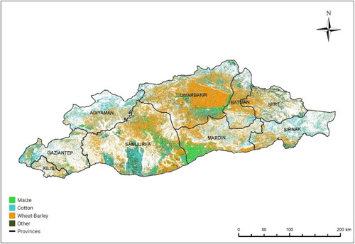
Our study area lies in the South-eastern Anatolia Region of Türkiye, consisting of Kilis, Gaziantep, Adiyaman, Sanliurfa, Mardin, Diyarbakır, Batman, Sirnak, and Siirt provinces (Figure 1). It covers the Euphrates-Tigris Basin and upper Mesopotamia plains, including the region of the Southeast Anatolia Project (with the Turkish acronym of GAP). The GAP region involves 22 dams, 19 hydroelectric power plants (HEPPs), and a total irrigation area of 1.8 million ha. The GAP project is vital with its extensive contributions to the economy, agricultural productivity, and new employment opportunities (URL 1, Sevinç et al. 2019). Approximately 4.5 million ha of land has been cultivated in the GAP region, which is 11.4% of the total cultivated area of Türkiye. Moreover, 55.12% of the total cotton and 32.48% of the whole wheat have been obtained from the GAP region (URL 2). The main crops grown in the region are wheat, wheat-barley, cotton, maize and others from national sources (Table 1, URL 3).

Figure 1. Location and mosaic image of the study area.

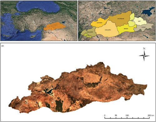
Table 1. The main crops grown in the study area.

	2005		2010		2020
Crop type	Cultivated area (da)	Production (ton)	Cultivated area (da)	Production (ton)	Cultivated area (da)	Production (ton)
Wheat	11,666,120	2,984,122	13,068,185	3,639,214	11,242,353	4,237,123
Wheat-Barley	6,432,070	1,765,814	4,496,170	1,057,188	3,639,418	1,044,877
Maize	1,018,340	585,057	1,396,143	1,344,038	2,477,532	3,434,537
Cotton	5,901,900	1,626,910	5,757,894	1,186,916	3,791,074	1,420,857

Source: URL 3.

Although the land cover mainly comprises agricultural lands, it also includes mountains, small urban areas, and wetlands. There are two main reasons for the selection of this region. The first is the increase in agricultural activities in the region with the GAP project implemented in 1989. Unfortunately, the increase in agricultural production triggers the application frequency of CRB. The second is that the agricultural diversity of the area is abundant. We believe that the emission results obtained in the study would provide an advantage in evaluating different crops of some national statistics (TSI 2020) and has the potential to support decision-making processes.

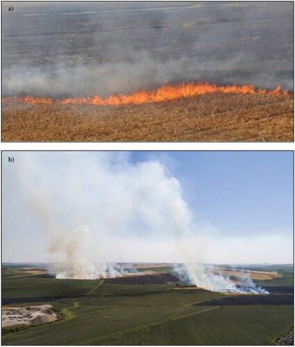
Crop Residue Burning (CRB) is one of the most common methods used worldwide, although it was forbidden officially. This practice has been employed not only in Türkiye (Figure 2) but also in other countries such as the United States (McCarty et al. 2007), China (Gao et al. 2017) and India (Singh et al. 2021). Farmers prefer CRB since it is fast and labour-free, and they also think it is an effective method to control pests and weeds and increase fertility. However, there are varying adverse effects of CRB locally and globally. Un-harvested land and healthy vegetation areas within CRB areas have been negatively affected, and traffic accidents occurred due to the smoke during the fire. Moreover, CRB results in the loss of organic matter on the topsoil, which is one of the main factors affecting the yield of agriculture, and it is essential to preserve a high amount of organic matter in the soil (Çıtak et al. 2006).

Figure 2. Some examples of CRB in the study area (Source: URL 4, URL 5).

2.2. Data

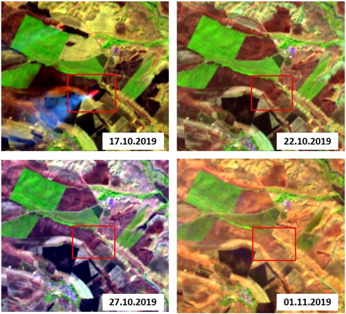
We used two different Sentinel satellites in this study, namely Sentinel-2 and Sentinel-5P belonging to Earth observation missions from the Copernicus Programme. Sentinel-2 satellites include two identical satellites, which are Sentinel-2A (launched on 23 June 2015) and Sentinel-2B (launched on 23 June 2015). These satellites provide 10 to 60 m spatial resolution data for 13 spectral bands within 5-day periods (ESA 2020). Most of the agricultural areas in Türkiye are fragmented and small; therefore, high spatial resolution is necessary to determine the boundaries of the agricultural parcels accurately. Another factor in the selection of the satellite is the temporal resolution since the burning effect of a field exposed to CRB disappears in different time periods. In our study area, for some of the agricultural parcels, CRB effect disappeared within 15 days; however, there are several cases in different parts of the world in which shorter time windows occurred even up to one day (Vadrevu et al. 2022). Therefore, frequent satellite images obtained from multi-sensor system are very important for CRB research. Afterwards, the related agricultural parcel seems like a traditional harvested area; therefore, satellites having a temporal resolution of one week or shorter would be desirable to find the CRB-affected regions precisely. We examined the spectral change of some agricultural parcels exposed to CRB during and after the practice using Sentinel-2A and 2B data (Figure 3). We observed that up to ten days after the residue burning, there are still indications of burning in the field represented by low spectral reflectance values. The image captured after the fifteenth day of CRB exhibits similar reflectance with an unburned field, making CRB detection impossible. Moreover, the cultivation and harvesting periods of crops vary for some regions and farmers, which affects the CRB application date. Therefore, frequent monitoring of agricultural areas is essential.

Figure 3. The temporal and spectral change of a field in Diyarbakır where CRB was applied.

The high spectral resolution of Sentinel-2 allows the opportunity to observe the crops’ phenological stages and use various remote sensing indices such as Normalized Difference Vegetation Index (NDVI), Normalized Difference Water Index (NDWI), Normalized Burned Ration Index (NBR), and difference of NBR (dNBR) (Table 2) (Bahsi et al. 2019; García-Llamas et al. 2019). We used Level 2 A products to minimize the geometric and atmospheric distortions (ESA 2020). Copernicus program has provided Level 2 A images globally since December 2018, in which atmospheric and radiometric corrections were implemented to eliminate or minimize the scattering, absorption, cloud, and haze effects. Level-2A products are also geometrically corrected and presented in a projection system (ESA 2020; Aksoy et al. 2022).

Table 2. Sentinel-2 bands used in various application parts of the study.

Section	Dates	Bands
Crop Type Mapping	Mid-July and Mid-September	RE-3 (B7), RE-1 (B5), Green (B3)
Burned Area Mapping	April-November period	NIR (B8), SWIR (B11)
Study Area Mosaic	August	Red (B4), Green (B3), Blue (B2)
Non-Agricultural Areas Masking	April-November period	NIR (B8), RED (B4)
Water Bodies Masking	April-November period	Green (B3), SWIR (B11)

We also used the Sentinel-5 Precursor (P) satellite data in this research. Sentinel-5P is the first Copernicus mission, developed to monitor the atmosphere with its TROPOspheric Monitoring Instrument (TROPOMI) instrument. TROPOMI measures the ultraviolet and visible (270–495 nm), near-infrared (675–775 nm) and shortwave infrared (2305–2385 nm) light with A temporal resolution of less than one day (URL 6). It was launched on 13 October 2017, and it became fully operational on 5 March 2019 after the commissioning phase ended (URL 7). The native spatial resolution of Sentinel-5P is 5.5*3.5 km. However, we used NO₂ productS of Sentinel-5P available in the GEE platform, and this product is resampled to approximately 1*1 km (URL 8). Sentinel-5P Level 2 products are streamed as the near-real-time (NRTI), the Non-Time Critical or Offline (OFFL) and the Reprocessing (RPRO). NRTI data becomes available within 3 h after data acquisition and is widely used for rapid operational processing (URL 9). We used Near Real-Time NO₂ Level 3 (NRTI/L3_NO₂) data available in the GEE platform, including gridded high-resolution imagery of NO₂ concentrations (URL 10). In this study, we generated Sentinel-5P NO₂ density maps, showing the total vertical column of NO₂ (ratio of the slant column density of NO₂ and the total air mass factor) (URL 11).

We visually analysed the active fire data from NASA’s Fire Information for Resource Management System (FIRMS), consisting of data from the NASA’s Moderate Resolution Imaging Spectroradiometer (MODIS) aboard the Aqua and Terra satellites and the Visible Infrared Imaging Radiometer Suite (VIIRS) aboard S-NPP and NOAA 20 (URL 14; Schroeder et al. 2014; Giglio et al. 2016). We evaluated the compliancy of FIRMS data with Sentinel-5P and burned agricultural fields that we identified from Sentinel-2 data.

3. Methods

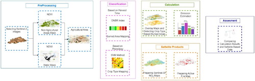
We conducted four steps in this study in the GEE platform: pre-possessing, classification, emission calculation, and satellite-based emission (Figure 4). First, we generated a complete mosaic image of the study area for August 2019. Then, we identified water and non-agricultural areas using various remote sensing indices and masked these regions from the mosaic image. After the masking, we used multi-temporal Sentinel-2 images selected based on the phenologic cycles of different crops and implemented the Support Vector Machines (SVM) classification (Vapnik et al. 1997). As a result, we created a crop type map consisting of maize, cotton, wheat-barley, and other classes. Besides, we used an extra set of Sentinel-2 satellite images, selected based on the harvest dates of different crop types to identify burned areas. Afterwards, we determined the burned agricultural lands in the region for 2019 using the dNBR index. Integrated usage of crop type maps and burned area maps let us conduct crop-specific emission calculations for the agricultural parcels exposed to residue burning. We employed the emission calculations following the Intergovernmental Panel on Climate Change (IPCC) standards. We estimated the emissions per crop and per province as spatial extent. Finally, to better analyse the emission calculation, we created maps of the NO₂ product of the Sentinel-5P satellite in the GEE platform and compared these maps with calculated values.

Figure 4. The flowchart of methodology.

3.1. Pre-processing

In the pre-processing, we first created the study area’s ortho-mosaic image covering 31 Sentinel-2A/B image frames for August 2019 (Figure 3). We then masked the non-agricultural areas using NDWI and NDVI indices to deal with only agricultural areas for the later stages and minimize uncertainties. First, we applied the NDVI index to all images for the April-November period and performed the visual analysis with different threshold values. As a result, we masked the non-agricultural areas based on a threshold value of 0.65, which was determined by evaluating the average NDVI value for well-known agricultural fields. Spectral reflectance values vary for different land categories; data acquisition conditions and diversity of geographical regions also impact the NDVI threshold. We employed the second masking process for water areas. We applied NDWI to images in a similar period and used the accepted value of 0.30 in the literature as the threshold value (Topaloğlu et al. 2021). Thus, we masked natural water bodies and waterways in the study area. We generated the crop type map after masking the water and non-agricultural areas.

3.2. Classification

Pixel-based (supervised and unsupervised) classification methods have been widely used to extract meaningful information from remote sensing data (such as crop type maps, yield maps, land cover and land use maps) (García-Llamas et al. 2019). Recently, machine learning methods have been used more frequently in the literature due to their ability to produce more accurate results than traditional methods (Demidova et al. 2019; Aksoy et al. 2022). We used the SVM method for the classification, which provides more accurate results than other pixel –based classification methods and requires very few samples (Mountrakis et al. 2011; Alganci et al. 2013). As with most machine learning methods, the SVM method uses unique training sets to adjust its parameters to solve the uncertainties in the classification. Thus, it learns how to classify unknown samples from the training data set. SVM is widely used in agricultural areas that are likely to show similar reflections since it makes classes separable (Mucherino et al. 2009; Alganci et al. 2013). Besides, SVM algorithms use mathematical parameters defined as kernels. The kernel takes the data as input and converts it into the required form. It uses different kernel types for different SVM algorithms. Linear, nonlinear, polynomial, sigmoid, and radial basis functions (RBF) are examples different kernel types. We used RBF in this study with gamma and a cost value of 128, and 64, respectively. After applying the grid search function in the GEE platform, we found these values, a hyperparameter optimization technique (Aksoy et al. 2022).

Cross-validation methods are such as Jack Knife Test, Boot-strapping, Monte Carlo Test, k-fold etc (Aksoy et al. 2022). We implemented the 5-fold cross-validation method to analyse the training and validation accuracy which divides the data set into two separate groups, training and validation, to quantify the accuracy of the classification (Saud et al. 2020).

3.2.1. Crop type mapping

The main crops grown in the region are maize, cotton, wheat, and barley (Bahsi et al. 2019). We carried out the classification considering the phenological stages of these crops. We specifically analyzed different phenological stages of maize and cotton while constructing our methodological steps and selecting the data acquisition times for satellite images. The first crucial phenological phase of the maize, tasselling stage, occurs before the flowering stage and maize exhibits higher spectral reflectance at this phase than other crops. As a result we used the satellite images of the tasselling stage for the classification. However, maize was planted in the region in two periods: the main and the second periods. Therefore, it is crucial to capture highly vegetated maize conditions for both periods, which also vary in different provinces of the region from north to south. We found appropriate times for each province in the literature for these two periods (Alganci et al. 2013; URL 12). In this context, we used July images to determine the main maize crop and mid-September images for the second maize crop. Besides, the tasselling phase is generally parallel to the pesticide phase that enables cotton to come out of the cones. Thus, cotton fields with pesticides can be easily distinguished from other crops due to the their whitish appearance on satellite images. Wheat-barley phenology is the opposite of the phenology of maize and cotton. Wheat and barley classes appear as empty fields when maize and cotton are cultivated. Finally, we classified the remaining pixels as the other class, those which do not exhibit any of the spectral characteristics mentioned above.

Considering the phenological characteristics, for each crop, we selected 25 samples from provinces with small areas and 50 from regions with larger provinces. Then, we produced a crop type map using the SVM method with a total of 1775 training data sets. We also conducted an independent accuracy assessment using test polygons for each class.

3.2.2. Burned area mapping

Determining the burn severity, defined as the magnitude of the ecological change caused by the fire (Petropoulos and Islam 2017), enables a more sensitive analysis of the burned area. Most satellite-based burn severity studies use methods based on remote sensing indices because they are easy to calculate and simple to implement. Spectral indices using the NIR and Short-Wave Infrared (SWIR) bands, such as Normalized Burn Ratio (NBR) and its bi-temporal version, the difference in Normalized Burn Ratio (dNBR), were used to detect the burned areas (Keeley 2009; García-Llamas et al. 2019). (1) $$\text{NBR = }\left(\text{NIR}-\text{SWIR}\right)\text{/}\left(\text{NIR+SWIR}\right)$$(1)

We generated NBR images for the selected periods and the formed dNBR images by taking the difference of May and November NBR images. We then spotted the burnt agricultural fields by taking the minimum NBR index value from the different days in May and created a complete pre-NBR mosaic image of the region. Then, we took the maximum NBR index value for each pixel from the different days in November and created a complete post-NBR mosaic image. Finally, we generated the dNBR index image by taking the difference between pre-NBR and post-NBR images to find the CRB exposed agricultural parcels and implemented threshold values widely accepted in the literature (Fang and Yang 2014). (2) $$\text{dNBR = }\left(\text{NBR}-\text{pre}\right)-\left(\text{NBR-post}\right)$$(2)

We performed an area-based accuracy assessment to evaluate the accuracy of the generated burned area map. First, we divided the burned area map into grids of 1 hectare (100 m × 100 m). Then, we randomly selected 200 grids, purely representing the related classes. We used the post-NBR image as a reference for visual comparison.

3.3. Emission calculation

We overlapped the burned area map and the crop type map to determine the crop type of burned agricultural fields. Then, we calculated crop-based emissions from CRB using Equations 1(1) $$\text{NBR = }\left(\text{NIR}-\text{SWIR}\right)\text{/}\left(\text{NIR+SWIR}\right)$$(1) and 2(2) $$\text{dNBR = }\left(\text{NBR}-\text{pre}\right)-\left(\text{NBR-post}\right)$$(2) proposed by the IPCC (IPCC 2020). (3) $$E=A*Mb*Cf*EF$$(3) (4) $$Mb=Y*s*d*pb$$(4)

Burned area (A) (decare) and Yield (Y) (kg/decare) information of each crop for 2019 were taken from the burned area map, and the national statistical report of the Turkish Statistical Institute (TSI 2020), respectively. The emission factors (EF) for NO₂, SO₂, CO, CO₂, CH₄ gases, and PM_2.5, PM₁₀ particles are taken from literature (Table 3). The EF of the wheat-barley class was calculated by taking the average of the values determined separately for both.

Table 3. Emission factors of greenhouse gases and PM from literature.

	CO	CO2	CH4	NO2	SO2	PM2.5	PM10
Maize	32.170^1	1363.000^6	1.930^3	0.140^5	0.440^5	4.950^1	5.170^1
Cotton	51.710^1	1375.000^3	3.270^3	0.220^7	1.570^8	6.890^1	7.220^1
Wheat-Barley	69.725^9	1189.500^9	1.970^9	0.045^9	0.594^9	5.425^9	5.650^9
Other	92.000^4	1515.000^4	2.700^4	2.800^8	1.170^8	3.900^4	8.500^2
Barley	83.360^1	1068.000^6	1.470^2	0.019^2	0.337^2	6.260^1	6.490^1
Wheat	56.090^1	1311.000^6	2.470^2	0.070^5	0.850^5	4.590^1	4.810^1

1. Jenkins et al. (1992). 2. Hayashi et al. (2014). 3. EPA (2014). 4. Santiago-De La Rosa et al. (2018). 5. Li et al. (2007). 6. Ni et al. (2015). 7. Cao et al. (2008). 8. McCarty et al. (2012). 9. Average wheat and barley values from the literature.

Also, the combustion factor (Cf), dry matter ratio (d), and the ratio between the mass of crop residues and the crop yield (s) values were obtained from the literature. These values were found for maize, cotton, and wheat-barley classes. However, when calculating the emission from the wheat – barley class, the values of wheat were used since the amounts determined for the two crops were similar. On the other hand, in the other class, these values could not be determined from past studies, and calculations were made by taking the average of the other three crop’s values (Table 4). Finally, since the proportion of burning residues (pb) value in the formula is about 1 (EEA 2016), it is not considered. Greenhouse gases and PMs emissions from CRB based on crop type were determined by calculation. Estimations were made for each province and values were collected to calculate the total emission in the study area.

Table 4. The values used for the parameters in the emission calculation.

	Maize	Cotton	Wheat Barley	Other
s	1.50^a	3.00^a	1.50^a	2.00^c
Cf	0.95^a	0.92^a	0.97^a	0.85^b
d	0.92^a	0.91^a	0.89^a	0.91^c

^aSantiago-De La Rosa et al. (2018). ^bMcCarty et al. (2012). ^cAverage of other crops.

3.4. Satellite based emission estimation

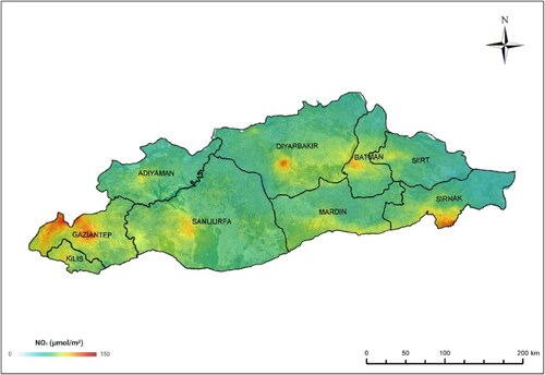
We created NO₂ density maps for June, July, and August when the harvesting is intense for different crop types. Besides, we produced a NO₂ density map for November following the local news on CRB applications in November. We generated monthly average values for NO₂ concentrations averaged over 30–31 days. After analysing minimum and maximum values of NO₂ concentrations for different months and operational NO maps provided by the Copernicus program (URL 13), we used the 0–150 micromole/m² range for our maps.

4. Results

4.1. Crop type mapping

We created a crop type map consisting of maize, cotton, wheat-barley, and other classes using the SVM method. Our results showed a total maize area of 2233.42 km², cotton of 10,378.85 km², 19,644.47 km² (wheat and barley), and 3090.82 km² other in the study area. Maize and cotton crops are mostly grown in the Sanliurfa province, and the wheat-barley class is grown in Diyarbakir (Figure 5).

Figure 5. Crop-type map of the study area.

We obtained the highest cross-validation result for the province of Sanliurfa (0.95) and the lowest values for Diyarbakır (0.81) (Table 5). We also conducted independent accuracy assessment using 25 test polygons for each class for the whole region. These polygons were different from the train and validation dataset used in cross-validation. We obtained high class-wise accuracy for different crops (Table 6).

Table 5. 5-fold cross validation results.

Province	Accuracy assessment results
Adiyaman	0.89
Gaziantep	0.93
Batman	0.86
Diyarbakır	0.81
Kilis	0.89
Mardin	0.92
Sanliurfa	0.95
Siirt	0.85
Sirnak	0.89

Table 6. Accuracy assessment of crop-type map.

Crop type	User’s accuracy	Producer’s accuracy
Maize	1	0.96
Cotton	0.98	0.83
Wheat	0.98	1
Other	0.84	0.99
Overall Accuracy: 0.95
Kappa Statistics: 0.93

4.2. Burned area mapping

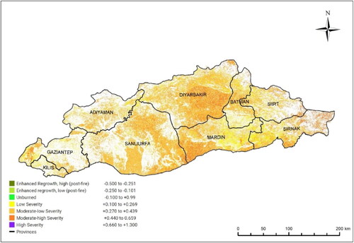
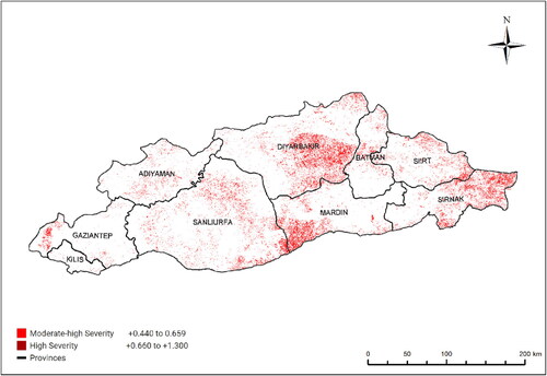
We used Sentinel-2A/B satellite images obtained before and after the harvest from May and November for the classification step. We used dNBR image to find out the spatial extent of burned agricultural parcels. dNBR values are generally suitable for the study area; but, we spotted some dark-coloured fields in the moderate low severity class. After carefully analysing each burnt severity class, we decided that Moderate-high severity (0.44–0.66) and High Severity (0.66-) classes successfully represented the burned areas (Figure 6). During our visual analyses, we used some agricultural parcels with burned smoke, easily seen in the Sentinel-2 images, and also benefitted from FIRMS active fire products. As a result of the study, we found 5063.52 km² of Moderate-high severity and 80.53 km² of high-severity burned area, and 31% of these were in Diyarbakır province, which was the highest. For Sanliurfa, Mardin, Sirnak, Siirt, Adiyaman, Batman, Gaziantep, and Kilis; the burnt area percentages were 19%, 15%, 10%, 5%, 4%, 3% and 1%, respectively. We found that burned areas spatially well matched with the agriculturally intensive areas in the crop-type map (Figure 6). We found some agricultural parcels for which simultaneous Sentinel-2 images acquired on the day of CRB practice were available. We concluded that high-severity burned areas represent these occasions based on these images. On the other hand, moderate-high severity areas were mostly for those agricultural parcels whose image was taken about a week after being burned. Since the possibility of having a simultaneous image with the CRB date is low, the area of the high severity class was less than the other class (Figure 6). The total emission caused by the maize residue burning was higher than that of other crops. The same result was also obtained by Dennis et al. (2002). According to the results, it was determined that the burned area map had 87% overall accuracy and 0.73 kappa value.

Figure 6. Burned area mapping of the study.

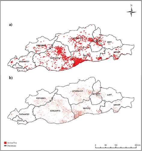
We downloaded FIRMS active fire data of the study region for 1 March − 30 November 2019 period and visually compared this map with the determined CRB-exposed areas (Figure 7). These two maps, in general, spatially matched and we observed that Sanliurfa, Diyarbakir and Mardin provinces had higher similarities in both maps. NASA’s Fire information for resource management systems (FIRMS) consists of satellite fire products from MODIS (Giglio et al. 2016) and Visible Infrared Imaging Radiometer Suite (VIIRS) (Schroeder et al. 2014) active fire detection products. The spatial resolutions of MODIS and VIIRS are 1000 m and 375 m, respectively.

Figure 7. FIRMS active fire data of the study region for 1 March–30 November 2019 period (a) Modis based active fire data (b) VIRS based active fire data (URL 14).

4.3. Emission estimation

In the study area, we found that 14,444.307 Gg greenhouse gas and 117.809 Gg PMs were released due to CRB in 2019. Our results showed that CO₂ and CO values were higher than other gases and PMs (Table 7). For the whole region, PM emissions were primarily due to maize and cotton burning. Most of the CH₄ emissions were caused by cotton burning. In addition, our crop-based total emission analysis illustrated that residue burning of maize caused the highest emission (5863.58 Gg), while wheat-barley caused the lowest emission (2129.40 Gg). The total emission from the cotton burning was 4437.98 Gg.

Table 7. Crop based emission amount of different gases and PMs in GAP region (Gg).

	CO	CO2	CH4	NO2	SO2	PM25	PM10	Total
Maize	133.99	5676.98	8.04	0.58	1.83	20.62	21.53	5863.58
Cotton	158.82	4223.05	10.04	0.64	4.55	19.96	20.92	4437.98
Wheat-Barley	116.64	1989.87	3.30	0.07	0.99	9.08	9.45	2129.40
Other	120.58	1985.70	3.54	3.55	1.53	5.11	11.14	2131.16
Total	530.03	13,875.61	24.92	4.84	8.91	54.77	63.04	14,499.07

4.3.1 Province based emission estimation results

The province-based emissions analysis showed that the highest amount was released in Diyarbakır, whereas the lowest was in Kilis. We examined the emission amounts of all gases and PMs for each provinces based on crop types (Table 8). In Adiyaman, we observed that the highest emission of 263.42 Gg was released from CO2 gas due to cotton residue burning. In contrast, CO₂ emissions of maize, wheat-barley and other crops were 64.81 Gg, 7.14 Gg, and 36.52 Gg, respectively (Table 8).

Table 8. Crop based emission amount of different gases and PMs (Gg) in Adiyaman.

	CO	CO2	CH4	NO2	SO2	PM25	PM10	Total
Maize	1.515	64.208	0.091	0.007	0.021	0.233	0.244	66.32
Cotton	9.906	263.418	0.626	0.004	0.027	0.120	0.126	274.23
Wheat-Barley	0.419	7.141	0.012	0.000	0.004	0.033	0.034	7.64
Other	2.218	36.519	0.065	0.067	0.028	0.094	0.205	39.20
Total	14.06	371.29	0.79	0.08	0.08	0.48	0.61	387.39

We determined that the total amount of emission due to CRB was 559.28 Gg in Gaziantep; the highest contribution was for CO₂ (531.25 Gg) primarily caused by cotton burning, similar to the Adiyaman case. In Gaziantep, most of the emissions were caused by cotton burning, followed by maize and other crops burning. Emission amounts caused by CO and CO₂ were higher compared to other gases and PMs (Table 9).

Table 9. Crop based emission amount of different gases and PMs (Gg) in Gaziantep.

	CO	CO2	CH4	NO2	SO2	PM25	PM10	Total
Maize	2.465	104.425	0.148	0.011	0.034	0.379	0.396	107.86
Cotton	11.305	300.618	0.715	0.048	0.343	1.506	1.579	316.11
Wheat-Barley	2.897	49.420	0.082	0.002	0.025	0.225	0.235	52.88
Other	4.663	76.789	0.137	0.142	0.059	0.198	0.431	82.42
Total	21.33	531.25	1.08	0.20	0.46	2.31	2.64	559.28

In Sanliurfa province, the primary cause of emissions was maize burning which released a total of 1863.74 Gg, with the highest proportion from CO2 (1804.43 Gg) and CO (42.59 Gg) (Table 10). Although the emissions caused by cotton burning were lower than the maize in the Sanliurfa region, total emissions caused by cotton burning were still higher compared to neighbourhood provinces such as Adiyaman, Gaziantep, Mardin, and Siirt.

Table 10. Crop based emission amount of different gases and PMs (Gg) in Şanlıurfa.

	CO	CO2	CH4	NO2	SO2	PM25	PM10	Total
Maize	42.589	1804.432	2.555	0.185	0.583	6.553	6.844	1863.74
Cotton	20.569	546.937	1.301	0.088	0.625	2.741	2.872	575.13
Wheat-Barley	20.613	351.654	0.582	0.013	0.175	1.604	1.670	376.31
Other	23.480	386.660	0.689	0.715	0.299	0.995	2.169	415.01
Total	107.25	3089.68	5.13	1.00	1.68	11.89	13.56	3230.19

In Mardin province, the primary source of emissions were maize and cotton residue burnings, respectively; whereas the wheat barley residue burning resulted in less CO₂ and CO gases produced higher emissions than other gases and PMs (Table 11).

Table 11. Crop based emission amount of different gases and PMs (Gg) in Mardin.

	CO	CO2	CH4	NO2	SO2	PM25	PM10	Total
Maize	65.365	2769.435	3.922	0.284	0.894	10.058	10.505	2860.46
Cotton	16.176	430.136	1.023	0.069	0.491	2.155	2.259	452.31
Wheat-Barley	17.351	296.003	0.490	0.011	0.148	1.350	1.406	316.76
Other	7.014	115.502	0.206	0.213	0.089	0.297	0.648	123.97
Total	105.91	3611.08	5.64	0.58	1.62	13.86	14.82	3753.50

When we analyzed the total emissions caused by different crop residue burnings in selected provinces, we concluded that Mardin and Sanliurfa were exposed to higher emissions primarily by maize and cotton residue burnings. Kilis found as the cleanest province in terms of CRB emissions and total emissions of CH₄, NO₂, and SO₂ were too low to be ignored.

Total emissions caused by maize residue burning were lower for Siirt, Sirnak and Kilis, whereas it reached the maximum for Mardin (2860.46 Gg) followed by Sanliurfa (1863.74 Gg), and Diyarbakir (800.16 Gg) (Table 12).

Table 12. Crop based total emisions (Gg) for each province.

Crop/Province	Adiyaman	Gaziantep	Batman	Kilis	Mardin	Urfa	Siirt	Sirnak	Diyarbakir
Maize	66.32	107.86	105.79	2.00	2860.46	1863.74	33.42	23.83	800.16
Cotton	274.23	316.12	177.40	10.24	452.31	575.13	417.66	1534.18	680.70
Wheat-Barley	7.64	52.88	104.81	5.99	316.76	376.31	153.42	119.48	992.11
Other	39.20	82.42	72.94	6.03	123.97	415.01	509.24	62.97	819.38
Total	387.39	559.28	460.95	24.26	3753.50	3230.19	1113.74	1740.46	3292.35

We found that wheat-barley residue burning resulted in the highest CO₂ emission in Diyarbakir compared to all other provinces.

In general, CO₂ emissions were high for all crops, followed by CO emissions, and in most cases, CH4-related emissions were higher than SO₂ and NO₂ emissions.

We found that maize and cotton are the primary crops causing the highest CO emissions. The NO₂ density was determined to be the lowest value in the wheat-barley and the highest value in the other class. The emission from cotton was very dominant in the distribution of SO₂. Finally, although the emissions of PMs from cotton, maize, and wheat-barley were similar, the PM₂₅ density resulting from the burning of the other was lower than PM₁₀ (Table 12).

4.4. Satellite based emission estimation

As mentioned in the previous sections, we calculated the monthly average NO₂ density maps for June, July, August and November using Sentinel-59 data by applying 0–150 micromole/m² range (Figure 8). We observed that the high-density areas in the NO₂ maps were consistent with where the CRB was applied (Figure 9).

Figure 8. The NO₂ maps for June, July, and August.

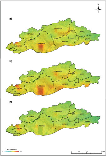
Figure 9. dNBR based burned areas.

Finally, we generated a Sentinel-5P NO₂ map for November to check the claims by the local people presented in the media regarding to the CRB cases in November. NO₂ concentration was found to be high in November (Figure 10), however it is not possible to say that it is precisely due to the CRB because of the cooling of the weather in November and the emission increase due to warming (Figure 10).

Figure 10. The N02 concentration of the region in November.

5. Discussion

The human impact on climate change has been clearly stated in the IPCC 6th Report (Marques et al. 2022, Nakaegawa and Murazaki 2022). Türkiye is located in the Mediterranean Basin, where vulnerability to climate change is very high. Therefore, human-induced fires such as residue burning and wildfires should be closely monitored since the extreme temperatures due to climate change trigger the occurrence and spread of fires. Within the scope of climate change adaptation and environmental policies, reducing emissions caused by greenhouse gases and particulate matter is significantly essential. Therefore, accurate identification of burned agricultural areas and calculation of CRB-related emission amounts are vital to cope with climate change and correctly determine air quality effects.

Moreover, it is also essential to obtain crop-based emission factors and phenological information to generate national-level reliable CRB-related emission estimations. We used the EF values published by Santiago-De La Rosa et al. (2018) and McCarty et al. (2012). Still, it is important to determine the region and crop-specific values for Türkiye in future studies.

We used Sentinel-2 images in this research to find the spatial distribution of agricultural areas, crop types and burned areas. We selected Sentinel-2 due to its 10 m spatial resolution compliance to determine small and fragmented agricultural parcels in our study region. In case of availability of large agricultural parcels, Landsat-8 and Landsat-9 images could also be integrated into implementation. Most of the studies in the literature used MODIS data for CRB determination due to its daily temporal resolution (Chen et al. 2017; McCarty et al. 2017; Lee et al. 2021; Kalluri et al. 2020). Although MODIS data could produce good results for large agricultural parcels, its spatial resolution is not sufficient to obtain high quality details, specifically for small and fragmented agricultural areas. Sentinel-2 satellites, with their high spectral and spatial resolution, provide an essential data set for CRB estimation; however, the number of CRB research with Sentinel-2 is quite limited (Ding et al. 2020). Deshpande et al. (2022) successfully used Sentinel-2 images for Central India to find burned agricultural areas; however, they did not conduct specific crop-based emission calculations. Instead, they estimated emissions assuming that all agricultural burning was due to wheat residue since wheat was one of the major winter crops for their area. Singh et al. (2021) used Sentinel-2 data to estimate CRB for the rice fields in the northern part of India. Our study region is large, 76458,9 km2, and includes different crop types and we estimated emissions due to different crop residue burning. The usage of the GEE platform provided an advantage to this work in terms of data processing time, dynamic access to the massive amount of satellite images, availability of several image processing functions and no requirement to download data.

The NO₂ density product of the Sentinel-5P satellite is generally helpful in finding hot spot areas exposed to high NO₂ releases. Although the satellite provides daily data, the loss of some data sets (CO, CH₄, and SO₂) in the study area is a disadvantage for detecting emissions of all greenhouse gases.

6. Conclusion

In this research, we determined the spatio-temporal distribution of crop types and burned areas due to CRB using Sentinel-2 images for a large region with diverse, fragmented agricultural parcels. We calculated crop-specific emissions caused by CRB using the EF values in the literature for maize, cotton, wheat and barley. The fact that the EF value, which varies depending on the country, region, and climate, had to be taken from the literature made it difficult to evaluate this study on a national scale; therefore, region-based determination of EF via field measurements should be conducted in future studies to have more precise emission estimations. We also used Sentinel-5P NO₂ density maps, MODIS and VIIRS active fire data to check the spatial matching of our results with these satellite-based products. MODIS and VIIRS spatial resolutions are insufficient to find small agricultural parcels exposed to burning.

Moreover, in some locations, fires did not occur, although there were indications in MODIS and VIIRS active fire data. Knowledge of the crop’s phenologic stages and periods and harvest time is also essential to accurately generate crop type maps and identify burned areas. Both high spatial and temporal resolution sensors are needed for CRB detection since fires might occur on small agricultural parcels and start quickly and last a short time. Therefore, integrating multi-sensor data to have high spatio-temporal coverage might be necessary to identify CRB-affected fields.

URL

URL 1, http://yayin.gap.gov.tr/dokumanflipbook/index.php?Dosya=756f4854d1 [accessed 2022 April]

URL 2, http://www.gap.gov.tr/tarim-sayfa-15.html [accesed 2022 January]

URL 3, http://www.gap.gov.tr/upload/dosyalar/pdfler/icerik/istatiski_veriler/Tarim_Istatistikleri.pdf.

URL 4, http://diyarbakir.csb.gov.tr/basin-duyurusu-aniz-yakilmasi-ile-ilgili-haber-64850 [accessed 2021 December]

URL 5, https://www.aa.5om.tr/tr/turkiye/guneydogu-ciftcisi-aniz-yakmaktan-vazgeciyor/1260742 [accessed 2022 August]

URL 6, https://docs.sentinel-hub.com/api/latest/data/sentinel-5p-l2/., accessed in September 2022

URL 7 https://sentinels.copernicus.eu/web/sentinel/missions/sentinel-5p [accessed 2022 September]

URL 8, https://developers.google.com/earth-engine/datasets/catalog/COPERNICUS_S5P_NRTI_L3_NO2#bands., accessed in August 2022

URL 9, http://www.tropomi.eu/data-products/level-2-products., accessed in September 2022

URL 10, https://developers.google.com/earth [accessed 2022 September] engine/datasets/catalog/COPERNICUS_S5P_NRTI_L3_NO2#bands [accessed 2022 September]

URL 11, https://developers.google.com/earth-engine/datasets/catalog/COPERNICUS_S5P_NRTI_L3_NO2#bands [accessed 2022 September]

URL 12, https://www.kalkinmakutuphanesi.gov.tr/assets/upload/dosyalar/e3bcdb695475747fe5edc444ecbb7f022994.pdf [accessed 2022 September]

URL 13, https://maps.s5p-pal.com/ [accessed 2022 September]

URL 14, https://www.earthdata.nasa.gov/learn/find-data/near-real-time/firms [accessed 2022]

Disclosure statement

No potential conflict of interest was reported by the author(s).

Additional information

Funding

Kübra Bahşi was supported by The Scientific and Technological Research Council of Türkiye (TUBITAK) within the scope of 2210C Master Scholarship program. We would like to thank TUBITAK for this support.

References

- Aksoy S, Yildirim A, Gorji T, Hamzehpour N, Tanık AG, Sertel E. 2022. Assessing the performance of machine learning algorithms for soil salinity mapping in Google Earth Engine Platform using Sentinel-2A and Landsat-8 OLI data. Adv Space Res. 69(2):1072–1086.
- Alganci U, Sertel E, Ozdogan M, Ormeci C. 2013. Parcel-level ıdentification of crop types using different classification algorithms and multi-resolution ımagery in Southeastern Turkey. Photogramm Eng Remote Sensing. 79(11):1053–1065.
- Bahsi K, Salli B, Kılıç D, Sertel E. 2019. Estimation of emissions from crop residue burning using remote sensing data. IJGW. 19(1/2):94–105.
- Behera MD, Mudi S, Shome P, Das PK, Kumar S, Joshi A, Rathore A, Deep A, Kumar A, Sanwariya C, et al. 2021. COVID-19 slowdown induced improvement in air quality in India: rapid assessment using Sentinel-5P TROPOMI data. Geocarto Int. 36:1–21. https://doi.org/10.1080/10106049.2021.1993351
- Cao G, Zhang X, Gong S, Zheng F. 2008. Investigation on emission factors of particulate matter and gaseous pollutants from crop residue burning. J Environ Sci. 20(1):50–55.
- Chakrabarti S, Khan MT, Kishore A, Roy D, Scott SP. 2019. Scott Risk of acute respiratory infection from crop burning in India: estimating disease burden and economic welfare from satellite and national health survey data for 250 000 persons. Int J Epidemiol. 48(4):1113–1124.
- Chauhan AJ, Johnston SL. 2003. Air pollution and infection in respiratory illness. British Med Bull. 68(1):95–112.
- Chen Z, Chen D, Zhuang Y, Cai J, Zhao N, He B, Gao B, Xu B. 2017. Examining the influence of crop residue burning on local PM2.5 concentrations in Heilongjiang Province using ground observation and remote sensing data. Remote Sens. 9(10):971.
- Çıtak S, Sönmez S, Öktüren F. 2006. Bitkisel Kökenli Atıkların Tarımda Kullanılabilme Olanakları. Derim. 23(1):40–53.
- Demidova LA, Klyueva IA, Pylkin AN. 2019. Hybrid approach to improving the results of the svm classifi-cation using the random forest algorithm. Procedia Comput Sci. 150:455–461.
- Dennis A, Fraser M, Anderson S, Allen D. 2002. Air pollutant emissions associated with forest, grassland, and agricultural burning in Texas. Atmos Environ. 36(23):3779–3792.
- Ding Y, Zhang H, Wang Z, Xie Q, Wang Y, Liu L, Hall CC. 2020. A comparison of estimating crop residue cover from Sentinel-2 data using empirical regressions and machine learning methods. Remote Sens. 12(9):1470.
- EEA (European Environment Agency). 2016. EMEP/EEA Air Pollutant Emission Inventory Guidebook 2016: technical guidance to prepare national emission inven-tories. EEA-Report; p. 21.
- ESA – Sentinel-5P Website. 2020. http://www.esa.int/Applications/Observing%7B%5C%7Dthe%7B%5C%7DEarth/Copernicus/Sentinel-5P.
- Fang L, Yang J. 2014. Atmospheric effects on the performance and threshold extrapolation of multi-temporal Landsat derived dNBR for burn severity assessment. Int J Appl Earth Obs Geoinf. 33:10–20.
- Gao R, Jiang W, Gao W, Sun S. 2017. Emission inventory of crop residue open burning and its high-resolution spatial distribution in 2014 for Shandong province, China. Atmos Pollut Res. 8(3):545–554.
- García-Llamas P, Suárez-Seoane S, Fernández-Guisuraga JM, Fernández-García V, Fernández-Manso A, Quintano C, Taboada A, Marcos E, Calvo L. 2019. Evaluation and comparison of Landsat 8, Sentinel-2 and Deimos-1 remote sensing indices for assessing burn severity in Mediterranean fire-prone ecosystems. Int J Appl Earth Obs Geoinf. 80:137–144.
- Giglio L, Schroeder W, Justice CO. 2016. The collection 6 MODIS active fire detection algorithm and fire products. Remote Sens Environ. 178:31–41.
- Glushkov I, Zhuravleva I, McCarty JL, Komarova A, Drozdovsky A, Drozdovskaya M, Lupachik V, Yaroshenko A, Stehman SV, Prishchepov AV. 2021. Spring fires in Russia: results from participatory burned area mapping with Sentinel-2 imagery. Environ Res Lett. 16(12):125005.
- Hayashi K, Ono K, Kajiura M, Sudo S, Yonemura S, Fushimi A, Saitoh K, Fujitani Y, Tanabe K. 2014. Trace gas and particle emissions from open burning of three cereal crop residues: ıncrease in residue moistness enhances emissions of carbon monoxide, methane, and particulate organic car-bon. Atmos Environ. 95:36–44.
- IPCC: The Intergovernmental Panel on Climate Change. 2020. https://www.ipcc.ch/documentation.
- Jenkins BM, Turn SQ, Williams RB. 1992. Atmospheric emissions from agricultural burning in California: de-termination of burn fractions, distribution factors, and crop-specific contributions. Agricult Ecosyst Environ. 38(4):313–330.
- Jethva H, Torres O, Field RD, Lyapustin A, Gautam R, Kayetha V. 2019. Connecting crop productivity, residue fires, and air quality over Northern India. Sci Rep. 9(1):16594.
- Kalluri ROR, Zhang X, Bi L, Zhao J, Yu L, Kotalo RG. 2020. Carbonaceous aerosol emission reduction over Shandong province and the impact of air pollution control as observed from synthetic satellite data. Atmos Environ. 222:117150.
- Keeley JE. 2009. Fire intensity, fire severity and burn severity: a brief review and suggested usage. Int J Wildland Fire. 18(1):116–126.
- Lee J-J, Lee J-B, Kim O, Heo G, Lee H, Lee D, Kim D-g, Lee S-D. 2021. Crop residue burning in Northeast China and its ımpact on PM2.5 concentrations in South Korea. Atmosphere. 12(9):1212.
- Li X, Wang S, Duan L, Hao J, Li C, Chen Y, Yang L. 2007. Particulate and trace gas emissions from open burning of wheat straw and corn stover in China. Environ Sci Technol. 41(17):6052–6058.
- Lin M, Begho T. 2022. Crop residue burning in South Asia: a review of the scale, effect, and solutions with a focus on reducing reactive nitrogen losses. J Environ Manage. 314:115104. .
- Marques AC, Veras CE, Rodriguez DA. 2022. Assessment of water policies contributions for sustainable water resources management under climate change scenarios. J Hydrol. 608(127690):127690. www.elsevier.com/inca/publications/store/5/0/3/3/4/3.
- McCarty JL. 2011. Remote sensing-based estimates of annual and seasonal emissions from crop residue burning in the contiguous United States. J Air Waste Manag Assoc. 61(1):22–34.
- McCarty JL, Ellicott EA, Romanenkov V, Rukhovitch D, Koroleva P. 2012. Multi-year black carbon emissions from cropland burning in the Russian Federation. Atmos Environ. 63:223–238.
- McCarty JL, Justice CO, Korontzi S. 2007. Agricultural burning in the Southeastern United States detected by MODIS. Remote Sens Environ. 108(2):151–162.
- McCarty JL, Krylov AM, Prishchepov A, Banach DM, Tyukavina A, Potapov PV, Turubanova S. 2017. Agricultural fires in European Russia, Belarus, and Lithuania and their impact on air quality, 2002 – 2012. In: Gutman G, Radeloff V, editors. Land-cover and land-use changes in eastern Europe after the collapse of the Soviet Union in 1991, Washington (DC): Springer; p. 193–221.
- Mountrakis G, Im J, Ogole C. 2011. Support vector machines in remote sensing: a review. ISPRS J Photogramm Remote Sens. 66(3):247–259.
- Mucherino A, Papajorgji P, Pardalos PM. 2009. A survey of data mining techniques applied to agriculture. Oper Res Int J. 9(2):121–140.
- Nakaegawa T, Murazaki K. 2022. Historical trends in climate indices relevant to surface air temperature and precipitation in Japan for recent 120 years.Int J Climatol. https://doi.org/10.1002/joc.7784
- Ni H, Han Y, Cao J, Antony Chen LW, Tian J, Wang X, Chow JC, Watson JG, Wang Q, Wang P, et al. 2015. Emission characteristics of carbona-ceous particles and trace gases from open burning of crop residues in China. Atmos Environ. 123:399–406.
- Petropoulos GP, Islam T. (Eds.). 2017. Remote sensing of hydrometeorological hazards. CRC Press, Taylor & Francis Group, Boca Raton.
- Santiago-De La Rosa N, Gonzalez-Cardoso G, Figueroa-Lara JDJ, Gutiérrez-Arzaluz M, Octaviano-Villasana C, Ramírez-Hernandez IF, Mugica-Alvarez V. 2018. Emission factors of atmospheric and climatic pollutants from crop residues burning. J Air Waste Manag Assoc. 68(8):849–865.
- Saud S, Jamil B, Upadhyay Y, Irshad K. 2020. Performance improvement of em-pirical models for estimation of global solar radiation in India: a k-fold cross-validation approach. Sustain Energy Technol Assessments. 40:100768. 2020.100768.
- Saxena P, Sonwani S, Srivastava A, Jain M, Srivastava A, Bharti A, Rangra D, Mongia N, Tejan S, Bhardwaj S. 2021. Impact of crop residue burning in Haryana on the air quality of Delhi. India Heliyon. 7(5):e06973.
- Schroeder W, Oliva P, Giglio L, Csiszar IA. 2014. The New VIIRS 375m active fire detection data product: algorithm description and initial assessment. Remote Sens Environ. 143:85–96.
- Sevinc G, Aydoğdu MH, Cançelik M, Sevinc MR. 2019. Farmers' attitudes toward public support policy o for sustainable agriculture in GAPSanliurfa, Turkey. Sustainability. 11(23):6617.
- Shinde R, Shahi DK, Mahapatra P, Singh CS, Naik SK, Thombare N, Singh AK. 2022. Management of crop residues with special reference to the on-farm utilization methods: a review. Ind Crops Prod. 181:114772. https://doi.org/10.1016/j.indcrop.2022.114772.
- Shen Y, Jiang C, Chan KL, Hu C, Yao L. 2021. Estimation of field-level NOx emissions from crop residue burning using remote sensing data: A case study in Hubei, China. Remote Sens. 13(3):404.
- Singh G, Kant Y, Dadhwal VK. 2009. Remote sensing of crop residue burning in Punjab (India): a study on burned area estimation using mulyi-sensor approach. Geocarto Int. 24(4):273–292.
- Singh D, Kundu N, Ghosh S. 2021. Mapping rice residues burning and generated pollutants using Sentinel-2 data over northern part of India. Remote Sens Appl: soc Environ. 22:100486.
- Sun Z, Zhu Q, Deng S, Li X, Hu X, Chen R, Shao G, Yang H, Yang G. 2022. Estimation of crop residue cover in rice paddies by a dynamic-quadripartite pixel model based on Sentinel-2A data. Int J Appl Earth Observ Geoinf. 106:102645.
- Topaloğlu RH, Aksu GA, Ghale YAG, Sertel E. 2021. High-resolution land use and land cover change analysis using GEOBIA and landscape metrics: a case of Istanbul, Turkey. Geocarto Int. 1–27, https://doi.org/10.1080/10106049.2021.2012273.
- TSI (The Turkish Statistical Institute). 2020. https://biruni.tuik.gov.tr.
- US Environmental Protection Agency. 2014. National Emissions Inventory (NEI) Documentation [2016].
- Vadrevu K, San-Miguel-Ayanz J, Roy D, Wooster M, Giglio L, Schroeder W, Csiszar I. 2022. Summary of the 5th GWIS & GOFC-GOLD Fire Implementation Team Meeting Stresa, Italy. NASA Earth Observer. 34(5):1–13.
- Vapnik V, Golowich S, Smola AJ. 1997. Support vector method for function approximation, regression estimation, and signal processing. Adv Neural Inf Process Syst. 9:281–287.
- Vijay Deshpande M, Pillai D, Jain M. 2022. Detecting and quantifying residue burning in smallholder systems: an integrated approach using Sentinel-2 data. Int J Appl Earth Obs Geoinf. 108:102761.
- Zhang H, Ye X, Cheng T, Chen J, Yang X, Wang L, Zhang R. 2008. A laboratory study of agricultural crop residue combustion in China: emission factors and emission inventory. Atmos Environ. 42(36):8432–8441.
- Zhang S, Zhao H, Wu Z, Tan L. 2022. Comparing the ability of burned area products to detect crop residue burning in China. Remote Sens. 14(3):693.