Modelling some stand parameters using Landsat 8 OLI and Sentinel-2 satellite images by machine learning techniques: a case study in Türkiye

Abstract

Remote sensing technologies have been extensively used in forest management in predicting stand parameters. The goal of this study is to use Landsat 8 and Sentinel-2 satellite images to estimate stand volume, basal area, number of trees, mean diameter, and top height. 180 temporary sample plots were taken in pure Crimean pine stands with varied structure. Reflectance, vegetation indices, and eight texture values were generated from Landsat 8 and Sentinel-2 satellite images. The stand parameters were modelled with the remotely sensed data using multiple linear regression, support vector machine, and deep learning techniques. The results showed that the support vector machine technique provided the highest level of model performance with 45^° orientation for number of trees (R² = 0.98, RMSE%=5.97) and 90^° orientation for basal area (R²=0.91, RMSE%=15.22). The results indicated that the texture values presented better results than the reflectance and the vegetation indices in estimating the stand parameters.

Keywords:

• Stand parameters
• remote sensing data
• multiple linear regression
• support vector machine
• deep learning

1. Introduction

Forests are the world’s largest terrestrial ecosystems and carbon storage pool, providing us with a variety of economic, ecological, and social benefits such as wood and non-wood products, biodiversity conservation, recreation as well as water and soil protection. (Eckert 2012; Xie et al. 2017). Gathering accurate and timely forest inventory data and monitoring the forest resources over time are essential components of sustainable forest management planning (Baskent et al. 2008; Sakıcı and Günlü 2018). Stand parameters such as number of trees, basal area, stand volume, stand mean diameter and stand top height are significant to evaluate forest resources (Lu et al. 2004). Forest structure is an important factor affecting many ecosystem values such as wood production, erosion control, soil protection, biodiversity, and water production. For sustainable forest management planning, the forest structure should be monitored and kept under control. For this reason, it’s critical for forest managers to determine stand parameters accurately and reliably in planning for sustainable forest management (Spies 1998; Özdemir and Karnieli 2011; Bolat et al. 2022). Individual trees in sample plots are measured to determine the critical forest stand parameters such as stand volume, basal area, number of trees, mean diameter and stand top height. Traditionally, forest stand parameter data have been collected mostly with field surveys, which are costly, time-consuming, and inefficient (Hyyppä et al. 2000). Remote sensing data have recently shown to be an excellent tool for evaluating and monitoring large forest areas and stand parameters with moderate accuracy (Hyyppä et al. 2000; Özdemir and Karnieli 2011; Mora et al. 2013).

There are various remote sensing data coming from the optical, lidar and radar data sources and, these are used to estimate some stand parameters (Shataee 2013; Yazdani et al. 2020). When the literature is examined, there are few studies focused on the estimation of stand parameters with different satellite images. For example, the stand volume was estimated with WorldView-2 (Özdemir and Karnieli 2011; Mohsin et al. 2021), SPOT-5 satellite image (Xie et al. 2017), airborne laser scanning (LIDAR) (Giannico et al. 2016; Rahlf et al. 2021) and ALOS PALSAR (SAR) (Long et al. 2020), the basal area with digital aerial images (Özkan and Demirel 2018), Landsat ETM+, Ikonos satellite image (St-Onge et al. 2008), the number of tress with Landsat ETM + data (Mohammadi et al. 2010), RapidEye imagery (Wallner et al. 2015), airborne laser scanning (Błaszczak-Bąk et al. 2022), the mean diameter with WorlView-2 imagery (Özdemir and Karnieli 2011), Landsat 8 OLI (Sakıcı and Günlü 2018), LIDAR data (Sačkov et al. 2019) and the stand top height was estimated with LIDAR data (Mora et al. 2013). Furthermore, optical, radar and lidar data are used to estimate stand parameters whether separately or jointly (Morin et al. 2019; Beaudoin et al. 2022). In addition to these, depending on the recent developments in unmanned aerial vehicle (UAV) technologies, some studies have been carried out to estimate stand parameters using images taken with these UAV (Liebermann et al. 2018; Krause et al. 2019; Kameyama and Sugiura 2020). There are also other research initiatives focusing on the estimation of stand parameters using optical, lidar and radar satellite data together (Morin et al. 2019; Beaudoin et al. 2022). The latter group of studies show that the reflectance rates, vegetation indices and texture properties obtained from satellite images are mostly used (Özdemir & Karnieli, 2011; Xie et al. 2017; Sakıcı and Günlü 2018; Turgut and Günlü 2022). Some other studies concentrating on the estimate of stand parameters using different window sizes obtained from different satellite images can also be encountered in the literature (Kayitakire et al. 2006; Steinmann et al. 2013; Meng et al. 2016; Zhao et al. 2018; Chrysafis et al. 2019). However, very few studies (Kayitakire et al. 2006; Zhou et al. 2017) have been conducted on the estimation of stand parameters using data obtained from different orientations (0°, 45°, 90°, and 135°) using satellite images.

When the studies are examined together, one can realize that the multiple linear regression (MLR) analysis is mainly used in estimating the stand parameters using satellite images (Gama et al. 2010; Kulawardhana et al. 2014; Sheridan et al. 2014). In the meantime, though, non-parametric machine learning models have recently gained popularity. Many machine learning algorithms, such as Support Vector Machine (SVM), K-nearest Neighbor (KNN), and Random Forest (RF), are able to show complex non-linear patterns, in contrast to the linear regression model (Fassnacht et al. 2014; Zhang et al. 2019). The Deep Learning (DL) method, which is a multi-layer artificial neural networks, is also used for variable estimation in forestry (Ogana and Ercanli 2022). It is obvious that different modeling techniques have been applied in the estimation of stand parameters in recent years depending on the development of the aforementioned modeling techniques. It has been revealed that there are some recent studies directed towards estimation of stand parameters with machine learning algorithms, especially the DL modelling techniques (Zhang et al. 2019). When the studies on the estimation of stand parameters using remote sensing data and different modeling techniques are evaluated, it can well be seen that the modeling performance obtained provide better results than the regression analysis in generally. In a study by Sakıcı and Günlü (2018), the relationships between the variables obtained from the Landsat 8 OLI satellite image and the stand parameters were modeled using different modeling techniques (MLR and ANN). As a result of the study, it was seen that the ANN modeling technique presented better results than MLR. Zhao et al. (2019) used nonparametric modelling techniques to predict forest stand parameters and found that random forest (RF) performed better than the SVM, ANN and classification and regression tree (CART). Wu et al. (2016) evaluated the K-nearest neighbor (KNN), RF, stochastic gradient boosting, stepwise linear regression and SVM to estimate aboveground biomass using Landsat satellite data and found that the RF is more accurate than the other modelling techniques. Ahmadi et al. (2020) predicted the stand volume, basal area, and stem density using Sentinel-2 imagery with generalized linear model (GLM), Bayesian additive regression trees (BART), KNN, and SVM. The results indicated that the BART had the best modeling performance in estimating the stand volume and basal area compared to other modelling techniques. Zhang et al. (2019) predicted the aboveground biomass using different modeling techniques (KNN, RF, Support Vector Regression, DL and MLR) and different remote sensing data (Landsat 8 and LIDAR data). When the results obtained in the study were examined, the deep learning modeling technique achieved the best modeling performances. According to Narine et al. (2019), the aboveground biomass was estimated using ICESat-2 and Landsat satellite images with two modeling (RF and DL) techniques. When the results obtained were evaluated, it was seen that the DL modeling technique presented better results than RF. Few studies with DL modeling technique have generally been used in studies for the estimation of aboveground biomass (García-Gutiérrez et al. 2016; Narine et al. 2019). The stand parameters that have recently been estimated using DL modeling techniques are tree height and stand volume (Liu et al. 2019; Lang et al. 2019; Cha et al. 2022). Liu et al. (2021) predicted the diameter at breast height, stand volume, tree height, and stand density using LIDAR data with DL modeling techniques. Although there are quiet of a few other studies (usually MLR analysis was used in studies) for the estimation of stand parameters using remote sensing data in Türkiye, not many of them is designed to estimate stands parameters with the deep learning modeling technique. Therefore, this study will lay out the basis for similar future studies on the estimation of stands parameters with deep learning technique.

The objectives of this study are (1) to calculate the stand volume, basal area, number of trees, stand mean diameter and stand top height from ground measurements for each sample plot, (2) to generate the reflectance values, vegetation indices and texture features obtained from Landsat 8 OLI and Sentinel-2 satellite imagery for each sample plot, (3) to compare of model and test performances of MLR, SVM and DL methods used to estimate stand parameters.

2. Materials and methods

2.1. Study area

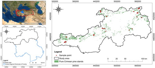
The case study was carried out in pure Crimean pine stands that spread within the borders of Ankara Regional Directorate of Forestry. The area covers 4,563,247 ha forests south to the Black Sea and within the Inner Anatolia Region, Türkiye. The area extends from 313096-598185 east longitudes to 4414251-4544558 north latitudes in WGS 1984 datum zone 36 according to UTM coordinate system (Figure 1). Within the case study area, pure Crimean pine stands cover around 136,985 ha. Elevation ranges from 239 m to 2541 m, an average of 1071 m above sea level and the average slope is 17%. The annual average temperature is 11.6 °C, the annual average highest and lowest temperature values are 17.9 °C and 5.5 °C, respectively. The average annual total precipitation amount is 400 mm. The study area is mainly composed of even-aged, pure stands of Crimean pine (Pinus nigra). Other common species in the study area are Pinus sylvestris, Pinus brutia, Abies nordmanniana, Fagus orientalis, Carpinus betulus, Quercus (Quercus cerris, Quercus infectoria, Quercus frainetto, Quercus robur, Quercus petraea), Cedrus libani, Juniperus sp. and Populus tremula.

Figure 1. Location of the study area.

2.2. Ground measurements

Ground measurements were conducted in 2019. A total of 180 sample plots was taken from pure Crimean pine stands covering five different site classes, six different age classes and three different closure classes in two replicates. The shape of the sample plots is in the form of a circle and the size of the sample plots varies between 400 and 800 m² depending on the stand crown closure (400 m² in fully closed stands (71–100%), 600 m² in medium closed stands (41–70%) and 800² m in low closed stands (11–40%).

In each sample plot, diameters at breast height were measured for all trees with a less than 8 cm diameter (in young stands) and greater than 8.0 cm at breast height. Mean age measurements were calculated from five trees close to the quadratic mean diameter in the sample plots. Height and age were measured in the dominant trees according to the 100 tallest trees per hectare, and then the site index of each sample plots was determined based on the site index table developed by Kalıpsız (1963). The volumes of trees in sample plot were calculated using the Equation (1)(1) $$v=0,000097\mathrm{ }x\mathrm{ }{d}_{1.3}^{1.740878}\mathrm{ }x\mathrm{ }{h}^{1.005521}$$(1) developed by Ercanlı (2020) for pure Crimean pine stands. The total volume was calculated by summing up the volumes of trees in each sample plot. The calculation of tree height, basal area, quadratic mean diameter and stand top height for sample plots were shown in the Equations (2)–(5). (1) $$v=0,000097\mathrm{ }x\mathrm{ }{d}_{1.3}^{1.740878}\mathrm{ }x\mathrm{ }{h}^{1.005521}$$(1) (2) $$h=1.3+\left(5.47\mathrm{*}{be}^{0.547}\right)\mathrm{*}{\left(1-e^{-0.042{\left(\frac{n}{ba}\right)}^{-0.360}\mathrm{*}{d}_{1.3}}\right)}^{0.648}$$(2) (3) $$\mathrm{ba}=\frac{\pi }{4}\times d_{1,3}^2$$(3) (4) $${\overline{\mathrm{d}}}_{\mathrm{g}}=\sqrt{\frac{{\overline{d}}_1^2+{\overline{d}}_2^2+\dots +{\overline{d}}_n^2}{\mathrm{n}}}$$(4) (5) $$h_{\mathit{top}}=\frac{h_1+h_2+\dots h_n}{n}$$(5) where $v$ is the volume of single tree in sample plot (m³), d_1.3 is the tree diameter measured at 1.30 m from the ground, h is the height of single tree in sample plot (m), be is site index value in sample plot (m), ba is the total basal area of sample plot (m²), n is number of trees in the sample plot, ${\overline{\mathrm{d}}}_{\mathrm{g}}$ is quadratic mean diameter (cm), and h_top is stand top height (m). Stand parameters such as V, BA and N per hectare value were calculated using the following Equations (6)–(8). (6) $$\mathrm{V}=\frac{10000}{A}\times v$$(6) (7) $$\mathrm{BA}=\frac{10000}{A}\times ba$$(7) (8) $$\mathrm{N}=\frac{10000}{A}\times n$$(8) where V is the stand volume (m³ ha⁻¹), BA is the stand basal area (m² ha⁻¹), N is the number of trees per hectare, and A is the sample plot area (m²). The descriptive statistics values of the stand parameters of the sample plots are given in Table 1.

Table 1. The descriptive statistics values of the stand parameters.

Stand parameters	Number of sample plot	Min.	Max.	Mean	St.D.
dg (cm)	180	2.0	56.3	27.0	10.72
htop (m)	180	3.0	36.3	16.9	7.09
N (number/ha)	180	137.5	6300.0	741.6	770.78
BA (m^2/ha)	180	1.97	91.44	32.05	15.56
V (m^3/ha)	180	10.00	1027.36	327.03	207.64

2.3. Remote sensing data

Landsat 8 Operational Land Imager (OLI) and Sentinel-2 satellite images were used as remote sensing data (USGS 2000). They were acquired in 2019 to match the acquisition time of the satellite images and the ground measurements. The seven bands of (Band 2, 3, 4, 5, 6, 7 and 8) Landsat 8 OLI and ten bands of (Band 2, 3, 4, 5, 6, 7, 8, 8 A, 11 and 12) Sentinel-2 satellite images were used. The reflectance, vegetation indices and texture values were generated from Landsat 8 OLI and Sentinel-2 images. The reflectance values were calculated for each band of satellite images using the QGIS 3.8.1 software. Some vegetation indices (Table 2) were calculated by using the reflectance values obtained from satellite images. The texture values were calculated separately for each band of Landsat 8 OLI and Sentinel-2, and eight different texture feature images such as mean (M), variance (VAR), homogeneity (HOM), contrast (CONT), dissimilarity (DIS), entropy (ENT), second moment (SM) and correlation (COR) were produced. Four different filters, 3 × 3, 5 × 5, 7 × 7 and 9 × 9, were used. Each filter was calculated separately for four different angles. This calculation is a function of distance (d) and angular (θ) relationship (P (i, j I d, θ)). It represents the probability of transition of gray levels from i to j. For distance (d) 1, matrices for angle degrees θ = 0° [1.0], 45° [1.1], 90° [0,1] and 135° [1,-1] were created. A total of 17 bands were used for Landsat 8 and Sentinel-2 satellites. Thus, a total of 2176 texture data sets were created for 17 bands, 8 textures, 4 filters and 4 different angles. The acquisition of texture data was carried out with the ENVI 5.2 program.

Table 2. Vegetation indices calculated from Landsat 8 OLI and Sentinel-2 satellite image.

Vegetation indices	Formula	Reference
NDWI (Normalized Difference Water Index)	(NIR – SWIR1) / (NIR + SWIR1)	(McFeeters, 1996)
MSI (Moisture Stress Index)	(SWIR1 / NIR)	(Hunt and Rock 1989)
PSSR (Pigment Specific Simple Ratio)	(NIR / RED)	(Blackburn 1998)
MID57	(SWIR1 + SWIR2)	(Lu et al. 2004)
VIS123	(BLUE + GREEN + RED)	(Lu et al. 2004)
ND73	(SWIR2 - RED) / (SWIR2 + RED)	(Lu et al. 2004)
GBNDVI (Green-Blue NDVI)	(NIR - (GREEN + BLUE)) / (NIR + (GREEN + BLUE))	(Wang et al., 2007)
MCARI (Modified Chlorophyll Absorption in Reflectance Index)	(( RedEdge1 - RED) − 0.2 x (RedEdge1 - GREEN)) x (RedEdge1 / RED)	(Haboudane et al. 2004)
CCCI (Canopy Chlorophyll Content Index)	(( NIR - RedEdge1) / (NIR + RedEdge1)) / ((NIR - RED) / (NIR + RED))	(Fitzgerald et al. 2010)
ChlGreen (Chlorophyll Green)	( NIRNarrow1 / GREEN) −1	(Gitelson et al. 2003)
SARVI (Soil and Atmospherically Resistant Vegetation Index)	(1.0 + L) x (NIR - (Rr - y x (RB - Rr))) / (NIR - (Rr - y x (RB - Rr)) + L) y = 0.735; Rr = 0.740; L = 0.487; RB = 0.560	(Kaufman and Tanre, 1992)

Sample plots were taken in the form of a circle in the field. The samples were spatially located around the sample plots’ centers in accordance with UTM coordinates collected by a handheld GPS tool. Then, depending on the size of the sample plots, appropriate radius of the sample plot (11.28 m for 400 m², 13.82 m for 600 m² and 15.96 m for 800 m²) was determined to establish the sampling areas as buffer zones. The reflectance, vegetation indices and textural features obtained from Landsat 8 OLI and Sentinel-2 satellite images were overlaid on the sample plots using GIS functions, and the values of each sample plot were calculated by taking the average of pixel values in the buffer zone for each sample plots.

2.4. Statistical analysis

Stand parameters and reflectance, vegetation indices and texture values obtained from satellite images were prepared for the modeling process. The dataset from the sample plots were randomly divided into two subgroups as training and testing based on data properties. 70% of the datasets (126 sample points) were used to the creation of models and 30% (54 sample points) for testing the models. The relationships between stand parameters and reflectance, vegetation indices and texture values using multiple linear regression analysis (MLR), support vector machines (SVM) and deep learning (DL) modeling techniques were investigated. In general, a high correlation can be observed among remotely sensed data such as reflectance, vegetation indices and texture values. The multiple linear stepwise regression analysis is a standard procedure and based on the inserting estimators into the model one at a time (Chong and Jun 2005; Ray‐Mukherjee et al. 2014). In this context, stepwise procedure of the MLR method was used for variable selection. The "frsftest" function, which is used to determine the predictive fit between independent variables, was used to obtain the univariate feature ranking using F test. The "fsrftest" function was applied in the MATLAB software. Also, the Taylor diagram (Taylor 2001), which is used to measure the correspondence between prediction and observation test data in terms of the root-mean-square error, Pearson correlation coefficient and the standard deviation, was presented for the sake of easier comparison. The radial distance from the origin of each point on the Taylor diagram indicates the standard deviation of the model estimates. The angular distance on the horizontal indicates the correlation coefficient between each predicted and observed stand parameters. The centered RMSE is indicated by the proximity or distance to the dashed line.

In the modeling process, (i) the MLR method was applied to determine the most appropriate independent variables among reflectance values, vegetation indices and texture datasets (Equation (9)), (ii) dependent and independent variables of MLR method were used as target and input variables of SVM and DL methods, respectively, (iii) the test data were run in the models created with the model dataset and (iv) the "paired t-test" was applied to determine whether there was a difference between the estimates of test prediction and observation data.

2.4.1. Multiple linear regression analysis

The MLR method was applied to determine the relationship between stand parameters (dependent variables) and reflectance, vegetation indices and texture values (independent variables). The MLR analysis was conducted using the software SPSS version 20. The statistical significance of the dependent and independent data was tested at 95% confidence level (Johnsson 1992).

2.4.2. Support vector machines

The SVM method, depending on statistical learning theory and structural risk minimization approach, was initially used to optimally separate the data to two classes. It was developed to solve the separation problem of multi-class and non-linear data. The aim is to obtain the optimal hyperplane that can separate the classes from each other. Different kernel functions can be used to create these limits, and the radial basis function was applied (Rodriguez-Galiano et al. 2015; Zhao et al. 2019). The "e1071" package in the "R" software was used to run the SVM method (Development Core Team R 2013; Meyer et al. 2015).

2.4.3. Deep learning

The DL method, which is a subset of traditional machine learning algorithms, is a kind of structurally complex artificial neural network. This method has been widely used, especially in image processing, virtual assistants, face recognition, driverless vehicles, translations, and image coloring. The framework of the DL consists of the input layer, hidden layers, and output layer. While there is one hidden layer in artificial neural networks, the DL method can be applied with more than one hidden layer. While the traditional neural network can only process a single hidden layer, the DL method can process the input data in its structure with multiple hidden layers. The input layer contains the arguments to be used for the modeling phase. One of the most important stages of the training phase is to determine the most appropriate hidden layer and the number of neurons. The adjective “deep” of this method is meant to refer to one hidden layer and the minimum number of hidden layers to be determined for its implementation was two. There are connections between all neurons, and each connection has a separate weight. Multi-layer perceptron, one of the algorithm types, was used in the implementation of the DL. Regularization, early stopping, and network reduction arguments were used to add useful variables to the model, adjust the learning speed, and avoid noisy learning, respectively. The "H2O" package in the "R" software is used to implement the DL method (Development Core Team R 2013; Aiello et al. 2015).

2.5. Model evaluation criteria

The criteria of correlation coefficient (r), the adjusted coefficient of determination (R²), mean absolute error (MAE), root mean square error (RMSE), the percentage RMSE (RMSE%) and the percentage bias (Bias%) were used in the evaluation of the MLR, SVM and DL models.

3. Results

3.1. Multiple linear regression analysis

The highest modeling performances with the reflectance and vegetation indices values were generated from the Sentinel-2 satellite image using MLR method (R²=0.44) and (R²=0.47) for V (m³), respectively (Table 3). Sentinel-2 satellite image outperformed according to Landsat 8 OLI in model performances related to texture values (Table 3). When the general evaluation was conducted, all the highest achievements were obtained with the texture values produced from the Sentinel-2 satellite image. According to the results of the applied MLR method, the highest modeling performance was achieved with the texture values. Especially, the data obtained from different orientations and window sizes contributed greatly to the modeling performance. Using different window size, the highest modeling performance for dg was achieved using the Sentinel-2 with a 9 × 9 filter with R²=0.60 (Table 3). For all other parameters, the highest modeling performance was obtained with the texture values produced for different orientations. The highest modeling performances were achieved for N with 45° [1, 0] (R²=0.82), BA (R²=0.72) and V (R²=0.79) with 90° [0, 1] and h_top (R²=0.72) with 135° [1, −1] texture data (Table 3). Variable importance rank for the outperforming MLR models obtained from Sentinel-2 satellite images was given in Figure 2. According to variable importance scores, "mean (M)" tissue data contributed the most to the models for dg, h_top, BA, and V, excluding N. The prediction and observation graphs of the MLR models applied to the model-test datasets were given in Figure 3.

Figure 2. Variable importance scores of the best MLR models based on Sentinel-2 sensor for dg (a), h_top (b), N (c), BA (d) and V (e).

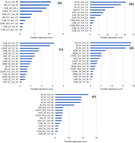
Figure 3. Observation and prediction graphs for test of MLR models obtained with texture values from Sentinel-2 data.

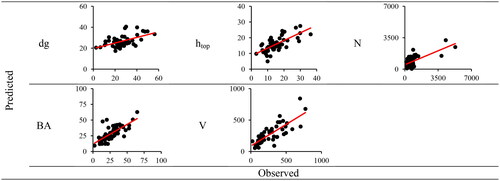
Table 3. The coefficient of determination for the MLR models of stand parameters.

Based on reflectance and vegetation indices	Stand parameter	Landsat 8 OLI				Sentinel-2
		Reflectance		Vegetation indices			Reflectance					Vegetation indices
	dg (cm)	0.23		0.25			0.23					0.20
	htop (m)	0.42		0.40			0.24					0.28
	N (number/ha)	0.15		0.17			0.14					0.16
	BA (m^2/ha)	0.34		0.42			0.41					0.45
	V (m^3/ha)	0.40		0.47		0.44						0.47
Based on texture window size	Stand parameter	Landsat 8 OLI				Sentinel-2
		3 × 3	5 × 5	7 × 7	9 × 9		3 × 3			5 × 5			7 × 7		9 × 9
	dg (cm)	0.43	0.38	0.42	0.42		0.58			0.54			0.59		0.60
	htop (m)	0.55	0.69	0.54	0.64		0.60			0.67			0.69		0.70
	N (number/ha)	0.60	0.63	0.33	0.34		0.72			0.67			0.80		0.79
	BA (m^2/ha)	0.40	0.56	0.57	0.50		0.60			0.65			0.71		0.66
	V (m^3/ha)	0.51	0.70	0.62	0.73		0.70			0.69			0.74		0.74
Based on texture orientations	Stand parameter	Landsat 8 OLI						Sentinel-2
		0°	45°	90°	135°				0°		45°			90°		135°
	dg (cm)	0.45	0.43	0.54	0.45				0.48		0.54			0.52		0.58
	htop (m)	0.62	0.70	0.64	0.51				0.66		0.69			0.67		0.72
	N (number/ha)	0.62	0.68	0.73	0.48				0.78		0.82			0.80		0.80
	BA (m^2/ha)	0.48	0.61	0.51	0.65				0.54		0.68			0.72		0.66
	V (m^3/ha)	0.67	0.68	0.60	0.66				0.70		0.76			0.79		0.74

Table 5. Model performance values obtained from 135° texture data of Sentinel-2 satellite image for h_top.

	Method	R^2	r	RMSE	RMSE%	Bias%	MAE	Paired t-test
Model	MLR	0.72	0.85	3.735	21.26	–0.56	2.873
	SVM	0.90	0.95	2.293	13.06	0.36	1.805	t	p
	DL	0.98	0.99	2.770	15.77	0.37	1.150
Test	MLR	0.51	0.71	4.834	30.87	–3.60	3.840	–0.823	0.414
	SVM	0.89	0.93	2.705	17.27	3.48	1.322	1.482	0.144
	DL	0.79	0.89	4.790	30.59	–19.50	4.010	–2.367	0.022

3.2. Support vector machine

The SVM method was applied to both the model and test data to which the MLR method was applied. In general, the SVM method presented very stable results for both model and test datasets (Figure 4). The difference between model-test performances in coefficient of determination (R²) does not exceed 0.01. The lowest performance of the SVM method was obtained for V (Model-Test R²= 0.85). To interpret whether there is an overfitting problem in machine learning techniques, the fit between model and test performances is very important. The SVM method has shown a high accuracy in terms of model-test performance criteria of stand parameters.

Figure 4. Observation and prediction graphs for test of SVM models obtained with texture values from Sentinel-2 data.

3.3. Deep learning

In the DL method, different layers and neuron numbers were tried for the network training phase (Figure 5). The highest performances were obtained from 7 layers and 80 neurons for dg, 10 layers and 70 neurons for h_top, 3 layers and 90 neurons for N, 10 layers and 80 neurons for BA, and 10 layers and 50 neurons for V. The selection of the outperforming layers and neuron numbers was performed according to the test results as an indicator of model-test fit and especially the response to independent data sets, rather than the model performance level. In this case, when the number of layers for N increased, the overall performance decreased. For BA, V and h_top, the increase in the number of layers positively affected the model performance. In the number of neurons, generally 50 and above increased the model performance.

Figure 5. The changes of correlation coefficients of model and test of dg, h_top, N, BA, and V according to the changing number of neurons and layers using the DL method.

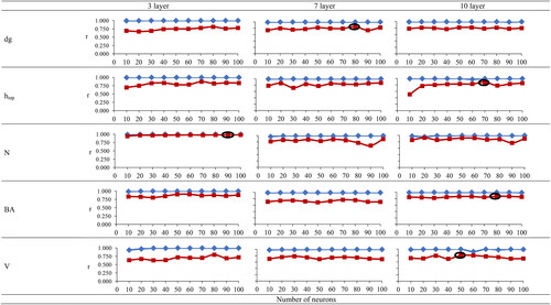
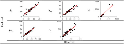
Model performance for all modeled parameters is quite high (Figure 6). Model and test performances in stand parameters are very close to each other. The stand parameter with which the model and test performance results are the closest is N (Model r = 0.99, Test r = 0.98).

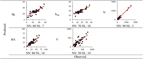
Figure 6. Observation and prediction graphs for testing of DL models obtained with texture values from Sentinel-2 data (NN: number of neurons, NL: number of layers).

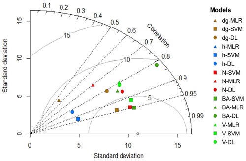
Taylor diagram was used to make an explanatory comparison regarding test evaluation (Figure 7). According to the Taylor diagram, the model with low standard deviation, low RMSE and high correlation coefficient was obtained for h_top by SVM method.

Figure 7. Taylor diagram which presents the geometric relationship among correlation coefficient, RMSE and standard deviation for comparison of model predictions.

3.4. Comparison of performance criteria of MLR, SVM and DL methods

Stand parameters were modeled using MLR, SVM and DL modelling techniques. In addition to comparing the model and test performances, the "paired t-test" was used to check whether the test predictions were compatible with the observation data. According to the test results, p > 0.05 indicates that the relevant model can be used with 95% confidence. Performance measures (R², r, RMSE, MAE) and paired t-test results for all estimates obtained with the applied techniques are presented in Tables 4–8. The results indicated that the highest model performance for the modeled dg was obtained with the DL method (R²=0.98, RMSE = 0.540 cm, RMSE%=1.99), and the highest test performance was obtained with the SVM method (R²=0.88, RMSE = 3.931 cm, RMSE%=14.85).

Table 4. Model performance values obtained from 9x9 filtered texture data of Sentinel-2 satellite image for dg.

	Method	R^2	r	RMSE	RMSE%	Bias%	MAE	Paired t-test
Model	MLR	0.60	0.78	6.652	24.50	0.24	5.219
	SVM	0.88	0.94	3.687	13.58	2.71	1.850	t	p
	DL	0.98	0.99	0.540	1.99	0.12	0.290
Test	MLR	0.30	0.55	9.184	34.70	–0.37	7.273	–0.074	0.941
	SVM	0.88	0.94	3.931	14.85	–3.25	2.692	–1.592	0.118
	DL	0.72	0.85	5.980	22.59	–1.92	4.750	–0.611	0.544

Table 6. Model performance values obtained from 45° texture data of Sentinel-2 satellite image for N.

	Method	R^2	r	RMSE	RMSE%	Bias%	MAE	Paired t-test
Model	MLR	0.82	0.91	281.722	39.47	0.08	205.585
	SVM	0.90	0.95	278.308	38.99	3.77	141.402	t	p
	DL	0.98	0.99	42.630	5.97	0.95	31.410
Test	MLR	0.49	0.70	694.747	87.46	–4.42	457.900	–0.365	0.716
	SVM	0.89	0.95	344.211	43.33	–1.84	107.921	–0.307	0.760
	DL	0.96	0.98	190.650	24.00	–2.34	141.030	–0.706	0.483

Table 7. Model performance values obtained from 90° texture data of Sentinel-2 satellite image for BA.

	Method	R^2	r	RMSE	RMSE%	Bias%	MAE	Paired t-test
Model	MLR	0.72	0.85	8.510	25.44	0.45	7.006
	SVM	0.91	0.96	5.092	15.22	–0.79	3.854	t	p
	DL	0.98	0.99	1.420	4.25	0.91	0.630
Test	MLR	0.70	0.84	7.243	25.23	–0.21	5.657	–0.056	0.955
	SVM	0.90	0.95	4.560	15.88	2.12	3.618	0.954	0.344
	DL	0.76	0.87	6.670	23.23	5.35	5.270	1.675	0.100

Table 8. Model performance values obtained from 90° texture data of Sentinel-2 satellite image for V.

	Method	R^2	r	RMSE	RMSE%	Bias%	MAE	Paired t-test
Model	MLR	0.79	0.89	98.031	28.44	0.35	78.709
	SVM	0.85	0.92	89.412	25.94	4.48	61.824	t	p
	DL	0.98	0.99	10.440	3.03	0.55	6.840
Test	MLR	0.64	0.80	107.227	38.58	0.59	82.895	0.109	0.914
	SVM	0.85	0.92	70.387	25.32	–0.97	40.674	–0.273	0.786
	DL	0.64	0.80	114.740	41.28	6.12	85.170	1.068	0.291

There was a model explanatory difference of 0.26 between the model and test performances obtained for the DL method. This difference was 0.30 in the MLR method, and the model-test performances in the SVM method were similar to each other. Considering the compatibility of the test estimates with the observation data, it was observed that the MLR method performed the most compatible estimate (p = 0.941). Although the model-test performances were similar, the SVM method was the lowest underperformed method in comparison with the test estimates (p = 0.118).

Among the modeling techniques applied in the modeling of h_top, the DL method showed the highest model performance (R²=0.98, RMSE = 2.770 m, RMSE%=15.77), while the highest test performance was in the SVM method (R²=0.89, RMSE = 2.705 m, RMSE%=17.27, Table 5). Although the modeling performance of the MLR method was the lowest, the model was found to present the best test-observation and estimation fit (p = 0.414). Considering the coefficient of determination for the DL method, while the test performance was (0.79), it was found to be inconsistent according to the observation and estimation results of the paired t-test (p = 0.022).

Among the techniques applied in modeling N, the DL method was found to present the method with the highest model and test performances (Table 6). Considering the model and test fit, the SVM method achieved the best modeling performance (Model R²=0.90, RMSE = 278.308 number/ha⁻¹, RMSE%=38.99, Test R²=0.89, RMSE = 344.211 number/ha⁻¹, RMSE%=43.33). In the MLR method, the test performance was quite low compared to the modelling performance (Model R²=0.82, RMSE = 281.722 number/ha⁻¹, RMSE%=39.47, Test R²=0.49, RMSE = 694.747 number/ha⁻¹, RMSE%=87.46). However, the test prediction and observation data of three methods were found to be compatible with each other. Considering the significance levels, it was observed that the method with the best test fit was SVM (p = 0.760).

Model and test performances for MLR and SVM, the methods used in modeling BA, were found to be compatible with each other (Table 7). Model and test achievements were the highest for DL and SVM methods, respectively. The method with the lowest model error was DL (R²=0.98, RMSE = 1.420 m²/ha⁻¹, RMSE%=4.25), and the method with the lowest test error was SVM (R²=0.90, RMSE = 4.560 m²/ha⁻¹, RMSE%=15.88). Although the modeling performance of the MLR method was lower than that of the other methods, its prediction accuracies were quite satisfactory in agreement with the observation data (p = 0.955).

Among the methods applied in modeling V, the SVM was the most compatible method for model and test performances (Table 8). On the other hand, the most inconsistent method with model and test performances was the DL method (Model R²=0.98, RMSE = 10.440 m³/ha⁻¹, RMSE%=3.03, Test R²=0.64, RMSE = 114.740 m³/ha⁻¹, RMSE%=41.28). Although the method with the highest predictive power was the SVM (R²=0.85, RMSE = 70.387 m³/ha⁻¹, RMSE%=25.32), the MLR (R²=0.64, RMSE = 107.227 m³/ha⁻¹, RMSE%=38.58), the DL method’s test performances (R²=0.64, RMSE = 114.740 m³/ha⁻¹, RMSE%=41.28) were similar with this model.

4. Discussion

4.1. Model success evaluation based on the satellite imagery

The modeling performance of estimating some stand parameters with Landsat 8 OLI and the Sentinel-2 satellite images using different modeling strategies was compared to each other. The results indicated that the models derived from the Sentinel-2 image achieved better modeling performances than the models obtained from the Landsat 8 OLI image. The Sentinel-2 satellite image with bands of different wavelengths and higher spatial resolution showed its advantageous over Landsat 8 OLI. The higher spatial resolution of the Sentinel-2 satellite ensured that the sample plots and pixel area were more compatible. Thereby, field and Sentinel-2 data could be better matched (Astola et al. 2019). When the results of the modeling of stand parameters with Sentinel-2 image were evaluated, the best accurate estimation was observed with the SVM method using the Sentinel-2 image’s 9 × 9 filtered texture data for dg (R²=0.88 and Test R²=0.88). Although the DL technique had a greater modeling performance (Model R²=0.98, Test R²=0.72), the SVM method presented a higher test performance, and the model-test performances were more compatible. For N modeled with 45° texture data, the best method was DL (Model R²=0.98, Test R²=0.96). For h_top modelled with 135° texture data, the best method was SVM (Model R²=0.90, Test R²=0.89). SVM was the best method for BA (Model R²=0.91, Test R²=0.90) and V (Model R²=0.85, Test R²=0.85) modeled with 90° texture data obtained from Sentinel-2 image. The texture data from the Sentinel-2 satellite image produced the best results in the estimation of stand parameters. Similar to our results, Chrysafis et al. (2019) estimated the stand volume with textural features of different windows of Sentinel-2 images. Mura et al. (2018) found Sentinel-2 satellite images to be more accurate than Landsat and RapidEye images for V prediction in two Italian test regions.

4.2. Evaluation of reflectance and vegetation indices data for modeling accuracy

Some researchers have used various satellite images for different tree species in modeling stand parameters with reflectance and vegetation indices values (Ateşoğlu 2009; Chrysafis et al. 2017). Özkan (2003) estimated the stand parameters such as dg, h, N, BA, and V by using the reflectance and vegetation indices obtained from the Spot 5 satellite image with the MLR method. The R² of the models obtained for dg, h, N, BA, and V with reflectance values were 0.50, 0.46, 0.23, 0.63, and 0.55, and with vegetation indices values were 0.32, 0.31, 0.26, 0.28, and 0.30, respectively. In the study conducted by Ateşoğlu (2009), the dg, h, N, BA, and V were predicted by using the Landsat 7 ETM + satellite image with the MLR method. By using reflectance values and vegetation indices together, the model R²values for dg, h, N, BA, and V were obtained as 0.24, 0.65, 0.33, 0.78 and 0.52, respectively. Chrysafis et al. (2017) predicted the V using Sentinel-2 and Landsat 8 OLI satellite images in their study. The highest performance was obtained with the reflectance values (R²=0.46) and vegetation indices (R²=0.52) obtained from the Sentinel-2 satellite image. In this study, reflectance and vegetation indices obtained from Landsat 8 OLI and Sentinel-2 satellite images were used in MLR models for dg, h_top, N, BA, and V. The highest model R²values for dg, h_top, N, BA, and V were found as 0.23, 0.42, 0.15, 0.41, and 0.44 with the reflectance and with vegetation indices data obtained from sentinel-2 satellite image 0.25, 0.40, 0.17, 0.45, and 0.47, respectively.

The characteristics of stand parameters, field structure, angle of incidence of the sun, acquisition time of the satellite images and the characteristics of satellite images greatly affect the modeling performance (Ateş and Demir 2009). According to the results obtained from the studies on the subject, vegetation indices achieved better modeling performances than reflection values in estimating stand parameters. Errors in the reflectance values detected by the satellite (shadiness, slope, sun angle, etc.) can weaken the penetration rate of the reflectance values of the detected region. Due to the consideration of band combinations in vegetation indices, the effect of these errors is minimized. In addition, the bands represent specific wavelengths. Since vegetation indices are combinations of bands with different wavelengths, they can better reflect the characteristics of the studied area. This makes vegetation indices more advantageous in estimating the stand parameters (Çil 2014).

4.3. Evaluation of texture data for modeling accuracy

When the studies in the literature on the subject are examined, despite many studies with data on texture features and different window sizes, there appears very few studies on the estimation of stand parameters using data on the different window size (3 × 3, 5 × 5, 7 × 7 and 9 × 9) and orientation (0°, 45°, 90°, 135°). Kayitakire et al. (2006) estimated h_top, N, and BA with the texture data obtained from the IKONOS-2 satellite image using MLR method. The R² of models were obtained 0.76, 0.82, and 0.35 for the h_top, N, and BA, respectively. Özdemir and Karnieli (2011) estimated the N, BA and V using the MLR method with the texture values produced from the WorldView-2 satellite image. The R² of models were found as 0.38, 0.54 and 0.42, respectively. In the study conducted by Sakıcı and Günlü (2018), they modeled the N, BA, V, and dg by using MLR and ANN methods by calculating texture values in different window sizes generated from Landsat 8 OLI satellite image. The R² of models obtained for N, BA, V, and dg were 0.18, 0.34, 0.33 and 0.40 for the MLR method, 0.61, 0.63, 0.65 and 0.59 for the ANN method, respectively. Chrysafis et al. (2019), estimated V with the texture data obtained from the Sentinel-2 satellite images. They examined the relationships between V and texture using different window sizes and orientations. The best performing result was obtained with 0° texture data with 3 × 3 window size (R²=0.91). Both our study (R²=0.85 for V) and Chrysafis et al. (2019; R²=0.91 for V) presented similar results. Kayitakire et al. (2006), Özdemir and Karnieli (2011) and Sakıcı and Günlü (2018) showed better prediction accuracies in their studies. The ANN method used by Sakıcı and Günlü (2018) increased the modelling performance. However, they achieved lower modeling performances compared to the performance level obtained with the different texture orientation data. Therefore, it has been observed that the texture orientation data can improve the estimation accuracy of the stand parameters.

Our results indicated that the inclusion of various independent variables in the model by using different window sizes and orientations and, the use of machine learning algorithms was quite effective in providing better prediction accuracies in estimating the stand parameters. Models with high performance levels were produced by determining the most suitable window sizes and orientations. The determination of the highest performing window size and orientation was decided by trial and error. Although it is not possible to generalize for the most appropriate window size and orientation in the estimations of stand parameters, it varies according to the field structure, stand characteristics and the technical characteristics of the sensor (Chrysafis et al. 2019). For example, Kayitakire et al. (2006) found that 15 × 15 window size for stand age and height, 5 × 5 window size for stand density, and 25 × 25 window size for stand basal area produced the accurate results with Ikonos satellite image. Meng et al. (2016) found the best correlation between the texture values in different window widths generated from the Spot-5 satellite image and the biomass with the 9 × 9 window size. Zhou et al. (2017) studied the correlations between the textural properties created by different window sizes (from 3 × 3 to 15 × 15) of the Quickbird satellite image and the leaf area index and found that the 3 × 3 window size produced the best results. In a study by Xie et al. (2017), the relationships between the texture values in various window sizes derived from the Spot-5 satellite image and the stand parameters were investigated. The accuracy in estimating the stand parameters first increased and then decreased with the increase of window size, with the best results obtained in the 9 × 9 window size. The texture features and vegetation indices produced for different window sizes (from 3 × 3 to 15 × 15) of the Spot-6 satellite image, as well as the relationships between their variables and the stand volume were investigated in a study by Zhou et al. (2020) and it was found that the best results were obtained in the 3 × 3 and 5 × 5 window sizes. In a study by Özkan and Demirel (2021) the relationships between the texture features produced for different window sizes (200, 400, 600, 800 and 1000 m²) of digital aerial image and WorldView-3 satellite images and stand volume, basal area, stem number and stand height in Crimean pine and oak stands were investigated. Their results showed that the ideal window sizes for V, BA, N, and h in Crimean pine stands were 100 m², 100 m², 1000 m², and 600 m², respectively, based on WorldView-3. The 800 m² window size was ideal for N and h, the 600 m² window size was optimal for V, and the 1000 m² window size was optimal for BA in the prediction based on the aerial images in Crimean pine stands. As stated in the studies above, the appropriate window size for predicting stand parameters varies depending on the composition of forest ecosystems and satellite images used.

The detection time of the satellites during the day is very important in determining the optimal window size and orientation value. The transit time of Landsat 8 OLI and Sentinel-2 satellites takes place in the morning hours in Türkiye (USGS 2000). Atmospheric conditions at these times, the direction of the sensor and the angle of incidence of the sun directly affect the structure of the data to be obtained (Ateşoğlu 2009). It is thought that the detection direction of the satellite images and the angle of incidence of the sun at that moment are effective in obtaining the highest performances at 45° and 90° using texture data in our study. When looking through the literature, it becomes clear that there aren’t enough studies examining the relationships between texture data produced using various orientations (0°, 45°, 90° and 135°) of different satellite images and stand parameters. In the literature, the appropriate window size varies in different forest ecosystems and satellite images in estimating the stand parameters. For example, Xie et al. (2017) stated that in examining the relationships between the texture values of different orientations derived from Quickbird satellite image and leaf area index, the lowest result was obtained at orientation of 45° and the best result at orientation of 90⁰. In the study conducted by Kayitakire et al. (2006), the stand age, stand height, basal area and stand density were best explained with an orientation of 45°, 0°, 45° and 90°, respectively. In another study by Chrysafis et al. (2019), the relationships between the spectral band, vegetation indices and texture characteristics obtained from the Sentinel-2 satellite image and V were investigated and the best relationship was found between the texture data obtained from the multi-seasonal spectrum at orientation of 0° and V.

4.4. Overall assessment of the model results

Two important points are observed in the results obtained in this study. The first is that although the test performance is high in the results of the DL method used for the estimation model, the test observation and estimation data are inconsistent according to the paired t-test. The second is that although both SVM and DL methods are machine learning techniques, a high difference is obtained between model-test performances only in the DL method. The R²value of the h_top is 0.98 for the model and 0.79 for the test with the applied MLR method. Although the coefficient of determination for the test predictions obtained is 0.79, the p value for the paired t-test is found to be 0.022 (p < 0.05) and the model network is found to be unusable.

In the modeling process, remote sensing data such as reflectance, vegetation indices and texture were used. The best performing result was achieved using texture data. The reasons for this result can be listed as using many texture data sets together and reflecting the texture properties of satellite images well by calculating for different window size, orientation, and functions (Pathak and Barooah 2013; Zheng et al. 2018). In the methods applied with texture data, the DL method for N and the SVM method for other parameters presented better prediction accuracies. Despite this result, the model performances of the DL method were higher for dg, h_top, BA, and V. Since the test performances were lower, the best method was chosen as SVM. The effect of the application process of SVM and DL methods is very important in obtaining the result in this way. The improvement argument (tuneResult) applied in addition to the kernel function used in the SVM method has ensured that the performance remains at a high level in the testing phase after the network training (Meyer et al. 2015). In the DL method, the arguments, activation function, number of neurons and number of layers determined by manual trial and error in the training process of the network both cause the training process of the network to prolong and make it difficult to reach the optimal estimations (Aertsen et al. 2010). Although the modeling performance is high for the DL method, the test performances remain at lower levels due to the difficulty of the network training process and the effect of the overfitting problem. All said, the SVM method is more user-friendly in terms of the application process and the improving arguments, providing quite similar results with higher model and test performance levels.

5. Conclusions

We studied the potential of reflectance, vegetation indices and textural features of Landsat 8 OLI and Sentinel-2 satellite image to predict the stand parameters such as V, BA, N, d_g and h_top. Based on the results the following conclusions can be drawn;

• When the model performances for the estimation of stand parameters derived from both satellite images were examined, it was indicated that the model performances obtained from the Sentinel-2 satellite imagery were higher.

• In the estimation of stand parameters, the texture features achieved better modeling performances than the reflectance and vegetation indices obtained from the Sentinel-2 satellite image.

• The best results were found for the d_g with 9x9 window size, for the N with 45° orientation, for the h_top with 135° orientation and, for the BA and V with 90° orientation.

• The optimal prediction models for stand parameters with the accuracy of estimating them were found as follows; the dg with SVM method (R²= 0.88, RMSE = 3.687 cm, RMSE%=13.58), the h_top with SVM method (R²=0.90, RMSE = 2.293 m, RMSE%=13.06), the N with DL method (R²=0.98, RMSE = 42.630 number/ha⁻¹, RMSE%=5.97), the BA with SVM method (R²=0.91, RMSE = 5.092 m² ha⁻¹, RMSE%=15.22) and the V with SVM method (R²=0.85, RMSE = 89.412 m³ ha⁻¹, RMSE%=25.94).

• Overall, this study indicated that the use of texture features instead of vegetation indices and spectral bands enhanced the model’s accuracy for estimating the dg, h_top, N, BA, and V in pure Crimean pine stands.

• Due to different forest ecosystems and satellite images, the ideal window size and orientation for estimating stand parameters using a textural feature of a remote sensing image may vary, and this needs to be investigated further.

Acknowledgements

The authors thank to the General Directorate of Forestry. Special thanks to Dr. Ferhat Bolat for his helping in the field work.

Disclosure statement

No potential conflict of interest was reported by the authors.

Additional information

Funding

This study was funded by the Scientific Research Project Unit of Çankırı Karatekin University (Grant No: OF061218D07).

References

- Aertsen W, Kint V, Van Orshoven J, Özkan K, Muys B. 2010. Comparison and ranking of different modelling techniques for prediction of site index in Mediterranean mountain forests. Ecol Modell. 221(8):1119–1130.
- Ahmadi K, Kalantar B, Saeidi V, Harandi EKG, Janizadeh S, Ueda N. 2020. Comparison of machine learning methods for mapping the stand characteristics of temperate forests using multi-spectral sentinel-2 data. Remote Sens. 12(18):3019.
- Aiello S, Kraljevic T, Maj P. 2015. Package ‘h2o. dim. 2:12.
- Astola H, Häme T, Sirro L, Molinier M, Kilpi J. 2019. Comparison of Sentinel-2 and Landsat 8 imagery for forest variable prediction in boreal region. Remote Sens Environ. 223:257–273.
- Ateş S, Demir E. 2009. Uzaktan algılamada çözünürlüğe bağlı veri kazanımı potansiyeli. TMMOB Harita ve Kadastro Mühendisleri Odası 12. Türkiye Harita Bilimsel ve Teknik Kurultayı, Ankara.
- Baskent EZ, Terzioğlu S, Başkaya Ş. 2008. Developing and implementing multiple-use forest management planning in Turkey. Environ Manage. 42(1):37–48.
- Beaudoin A, Hall RJ, Castilla G, Filiatrault M, Villemaire P, Skakun R, Guindon L. 2022. Improved k-NN mapping of forest attributes in Northern Canada using spaceborne L-band SAR, multispectral and biomass of urban forests using LiDAR. Remote Sens. 8:339.
- Błaszczak-Bąk W, Janicka J, Kozakiewicz T, Chudzikiewicz K, Bąk G. 2022. Methodology of calculating the number of trees based on ALS data for forestry applications for the area of samławki forest district. Remote Sens. 14(1):16.
- Bolat F, Ürker O, Günlü A. 2022. Nonlinear height-diameter models for Hungarian oak (Quercus frainetto Ten.) in Dumanlı Forest Planning Unit, Çanakkale/Turkey. Aust J For Sci. 139(3):199–220.
- Cha S, Jo HW, Kim M, Song C, Lee H, Park E, Lee WK. 2022. Application of deep learning algorithm for estimating stand volume in South Korea. J Appl Remote Sens. 16(2):024503.
- Chong IG, Jun CH. 2005. Performance of some variable selection methods when multicollinearity is present. Chemometr İntellig Labor Syst. 78(1-2):103–112.
- Chrysafis I, Mallinis G, Siachalou S, Patias P. 2017. Assessing the relationships between growing stock volume and Sentinel-2 imagery in a Mediterranean forest ecosystem. Remote Sens Lett. 8(6):508–517.
- Chrysafis I, Mallinis G, Tsakiri M, Patias P. 2019. Evaluation of single-date and multi-seasonal spatial and spectral information of Sentinel-2 imagery to assess growing stock volume of a Mediterranean forest. Int J Appl Earth Obs Geoinf. 77:1–14.
- Çil B. 2014. Bazı meşcere parametrelerinin farklı uydu görüntüleri yardımıyla tahmin edilmesi: Kelkit ve İğdir Planlama Birimi örneği. Trabzon: Karadeniz Teknik Üniversitesi, Fen Bilimleri Enstitüsü. p. 72 s. Yüksek Lisans Tezi,
- Eckert S. 2012. Improved forest biomass and carbon estimations using texture measures from WorldView-2 satellite data. Remote Sens. 4(4):810–829.
- Ercanlı İ. 2020. Ankara Orman Bölge Müdürlüğü Anadolu karaçamı meşcereleri için tek ağaç gövde çapı ve gövde hacminin uyumlu gövde çapı denklemleri ve yapay sinir ağları ile tahmin edilmesi. TÜBİTAK 119O061 nolu 1002 projesi.
- Fassnacht FE, Hartig F, Latifi H, Berger C, Hernández J, Corvalán P, Koch B. 2014. Importance of sample size, data type and prediction method for remote sensing-based estimations of aboveground forest biomass. Remote Sens Environ. 154:102–114.
- Fitzgerald G, Rodriguez D, O’Leary G. 2010. Measuring and predicting canopy nitrogen nutrition in wheat using a spectral index – the Canopy Chlorophyll Content Index (CCCI). Field Crops Res. 18–324.
- Gama FF, Dos Santos JR, Mura JC. 2010. Eucalyptus biomass and volume estimation using interferometric and polarimetric SAR data. Remote Sens. 2(4):939–956.
- García-Gutiérrez J, González-Ferreiro E, Mateos-García D, Riquelme-Santos JC. 2016. A preliminary study of the suitability of deep learning to improve LiDAR-derived biomass estimation. In: International Conference on Hybrid Artificial Intelligence Systems (pp. 588–596). Cham: Springer.
- Giannico V, Lafortezza R, John R, Sanesi G, Pesola L, Chen J. 2016. Estimating stand volume and above-ground LiDAR Data. Remote Sens. 14:1181.
- Gitelson AA, Gritz U, Merzlyak MN. 2003. Relationships between leaf chlorophyll content and spectral reflectance and algorithms for non-destructive chlorophyll assessment in higher plant leaves. J. Plant Physiol. 160(3):271–282.
- Haboudane D, Miller JR, Pattey E, Zarco-Tejada PJ, Strachan IB. 2004. Hyperspectral vegetation indices and novel algorithms for predicting green LAI of crop canopies: modeling and validation in the context of precision agriculture. Remote Sens. Environ. 90:337–352.
- Hunt Jr ER, Rock BN. 1989. Detection of changes in leaf water content using near-and middle-infrared reflectances. Remote Sens. Environ. 30(1):43–54.
- Hyyppä J, Hyyppä H, Inkinen M, Engdahl M, Linko S, Zhu YH. 2000. Accuracy comparison of various remote sensing data sources in the retrieval of forest stand attributes. For Ecol Manage. 128(1-2):109–120.
- Johnsson T. 1992. A procedure for stepwise regression analysis. Stat Pap. 33(1):21–29.
- Kalıpsız A. 1963. Türkiye’de karaçam meşcerelerinin tabii bünyesi ve verim kudreti üzerine araştırmalar. İstanbul: OGM yayını; p. 141.
- Kameyama S, Sugiura K. 2020. Estimating tree height and volume using unmanned aerial vehicle photography and SfM technology, with verification of result accuracy. Drones. 4(2):19.
- Kaufman YJ, Tanre D. 1992. Atmospherically resistant vegetation index (ARVI) for EOS-MODIS. IEEE Trans. Geosci. Remote Sens. 30(2):261–270.
- Kayitakire F, Hamel C, Defourny P. 2006. Retrieving forest structure variables based on image texture analysis and IKONOS-2 imagery. Remote Sens Environ. 102(3-4):390–401.
- Krause S, Sanders TGM, Mund JP, Greve K. 2019. UAV-based photogrammetric tree height measurement for intensive forest monitoring. Remote Sens. 11(7):758.
- Kulawardhana RW, Popescu SC, Feagin RA. 2014. Fusion of lidar and multispectral data to quantify salt marsh carbon stocks. Remote Sens Environ. 154:345–357.
- Lang N, Schindler K, Wegner J. 2019. Country-wide high-resolution vegetation height mapping with Sentinel-2. Remote Sens. Environ. 233:111347.
- Liebermann H, Schuler JL, Strager MP, Henntz AK, Maxwell AE. 2018. Using unmanned aerial systems for deriving forest stand characteristics in mixed hardwoods of West Virginia. J Geospat Appl Nat Resour. 2(1):1–12.
- Liu H, Shen X, Cao L, Yun T, Zhang Z, Fu X, Chen X, Liu F. 2021. Deep learning in forest structural parameter estimation using airborne LiDAR Data. IEEE J Sel Top Appl Earth Observ Remote Sens. 14:1603–1618.
- Liu J, Wang X, Wang T. 2019. Classification of tree species and stock volume estimation in ground forest images using Deep Learning. Comput Electron Agric. 166:105012.
- Long J, Lin H, Wang G, Sun H, Yan E. 2020. Estimating the growing stem volume of the planted forest using the general linear model and time series quad-polarimetric SAR ımages. Sensors. 20(14):3957.
- Lu D, Mausel P, Brondı́zio E, Moran E. 2004. Relationships between forest stand parameters and Landsat TM spectral responses in the Brazilian Amazon Basin. For Ecol Manage. 198(1-3):149–167.
- McFeeters SK. 1996. The use of Normalized Difference Water Index (NDWI) in the delineation of open water features. Int. J. Remote Sens. 17(7):1425–1432.
- Meng J, Li S, Wang W, Liu Q, Xie S, Ma W. 2016. Estimation of forest structural diversity using the spectral and textural information derived from SPOT-5 satellite images. Remote Sens. 8(2):125.
- Meyer D, Dimitriadou E, Hornik K, Weingessel A, Leisch F. 2015. e1071: misc Functions of the Department of Statistics, Probability Theory Group (Formerly: e 1071). TU Wien. R package version, 1.6-7.
- Mohammadi J, Joibary SS, Yaghmaee F, Mahiny AS. 2010. Modelling forest stand volume and tree density using Landsat ETM + data. Int J Remote Sens. 31(11):2959–2975.
- Mohsin AF, Suratman MN, Zakaria SAKY. 2021. Modelling of stand volume of Eucalyptus plantations using WorldView-2 Imagery in Sabah, Malaysia. ASM Sci J. 14(1):118–125.
- Mora B, Wulder MA, White JC, Hobart G. 2013. Modeling stand height, volume, and biomass from very high spatial resolution satellite imagery and samples of airborne LiDAR. Remote Sens. 5(5):2308–2326.
- Morin D, Planells M, Guyon D, Villard L, Mermoz S, Bouvet A, Thevenon H, Dejoux J, Toan TL, Dedieu G. 2019. Estimation and mapping of forest structure parameters from open access satellite images: development of a generic method with a study case on coniferous plantation. Remote Sens. 11(11):1275.
- Mura M, Bottalico F, Giannetti F, Bertani R, Giannini R, Mancini M, Orlandini S, Travaglini D, Chirici G. 2018. Exploiting the capabilities of the Sentinel-2 multi spectral instrument for predicting growing stock volume in forest ecosystems. Int J Appl Earth Obs Geoinf. 66:126–134.
- Narine LL, Popescu SC, Malambo L. 2019. Synergy of ICESat-2 and Landsat for mapping forest aboveground biomass with deep learning. Remote Sens. 11(12):1503.
- Ogana FN, Ercanli I. 2022. Modelling height-diameter relationships in complex tropical rain forest ecosystems using deep learning algorithm. J For Res. 33(3):883–898.
- Özdemir İ, Karnieli A. 2011. Predicting forest structural parameters using the image texture derived from WorldView-2 multispectral imagery in a dryland forest. Israel. International Journal of Applied Earth Observation and Geoinformation. 13(5):701–710.
- Özkan UY, Demirel T. 2018. Estimation of forest stand parameters by using the spectral and textural features derived from digital aerial images. Appl Ecol Env Res. 16(3):3043–3060.
- Özkan UY, Demirel T. 2021. The ınfluence of widow size on remote sensing-based prediction of forest structural variables. Ecol Process. 10(1):60.
- Özkan UY. 2003. Uydu görüntüleri yardımıyla meşcere parametrelerinin kestirilmesi ve orman amenajmanında kullanılması olanakları İstanbul: İstanbul Üniversitesi, Orman Fakültesi, Fen Bilimleri Enstitüsü; p. 70. s., Yüksek lisans Tezi.
- Pathak B, Barooah D. 2013. Texture analysis based on the gray-level co-occurrence matrix considering possible orientations. Int J Adv Res Electr Electron Instrum Eng. 2(9):4206–4212.
- Rahlf J, Hauglin M, Astrup R, Breidenbach J. 2021. Timber volume estimation based on airborne laser scanning comparing the use of national forest inventory and forest management inventory data. Ann For Sci. 78(2):1–14.
- Ray‐Mukherjee J, Nimon K, Mukherjee S, Morris DW, Slotow R, Hamer M. 2014. Using commonality analysis in multiple regressions: a tool to decompose regression effects in the face of multicollinearity. Methods Ecol Evol. 5(4):320–328.
- Rodriguez-Galiano V, Sanchez-Castillo M, Chica-Olmo M, Chica-Rivas M. 2015. Machine learning predictive models for mineral prospectivity: an evaluation of neural networks, random forest, regression trees and support vector machines. Ore Geol Rev. 71:804–818.
- Sačkov I, Scheer Ľ, Bucha T. 2019. Predicting forest stand variables from airborne LiDAR data using a tree detection method in Central European forests. Lesnicky Casopis. 65(3-4):191–197.
- Sakıcı OE, Günlü A. 2018. Artificial intelligence applications for predicting some stand attributes using Landsat 8 OLI satellite data: a case study from Turkey. Appl Ecol Env Res. 16(4):5269–5285.
- Shataee S. 2013. Forest attributes estimation using aerial laser scanner and TM data. Forest Syst. 22(3):484–496.
- Sheridan RD, Popescu SC, Gatziolis D, Morgan CL, Ku NW. 2014. Modeling forest aboveground biomass and volume using airborne LiDAR metrics and forest inventory and analysis data in the Pacific Northwest. Remote Sens. 7(1):229–255.
- Spies TA. 1998. Forest structure: a key to the ecosystem. Northwest Sci. 72:34–36.
- Steinmann K, Mandallaz D, Ginzler C, Lanz A. 2013. Small area estimations of proportion of forest and timber volume combining Lidar data and stereo aerial images with terrestrial data. Scand J For Res. 28(4):373–385.
- St-Onge B, Hu Y, Vega C. 2008. Mapping the height and above-ground biomass of a mixed forest using LiDAR and stereo Ikonos images. Int J Remote Sens. 29(5):1277–1294.
- Taylor KE. 2001. Summarizing multiple aspects of model performance in a single diagram. J Geophys Res. 106(D7):7183–7192.
- Turgut R, Günlü A. 2022. Estimating aboveground biomass using Landsat 8 OLI satellite image in pure Crimean pine (Pinus nigra JF Arnold subsp. pallasiana (Lamb.) Holmboe) stands: a case from Turkey. Geocarto Int. 37(3):720–734.
- USGS 2000. USGS earth explorer. https://earthexplorer.usgs.gov/.
- Wallner A, Elatawneh A, Schneider T, Knoke T. 2015. Estimation of forest structural information using RapidEye satellite data. Forestry: Int J For Res. 88(1):96–107.
- Wang F, Huang J, Tang Y, Wang X. 2007. New vegetation index and its application in estimating leaf area index of rice. Rice Sci. 14(3):195–203.
- Wu C, Shen H, Shen A, Deng J, Gan M, Zhu J, Xu H, Wang K. 2016. Comparison of machine-learning methods for above-ground biomass estimation based on Landsat imagery. J Appl Remote Sens. 10(3):035010.
- Xie S, Wang W, Meng J, Zhao T, Huang G. 2017. Estimation of forest stand parameters using SPOT-5 satellite images and topographic information. Preprints. https://doi.org/10.20944/preprints201710.0017.v1
- Yazdani M, Jouibary SS, Mohammadi J, Maghsoudi Y. 2020. Comparison of different machine learning and regression methods for estimation and mapping of forest stand attributes using ALOS/PALSAR data in complex Hyrcanian forests. J Appl Rem Sens. 14(02):1.
- Zhang L, Shao Z, Liu J, Cheng Q. 2019. Deep learning based retrieval of forest aboveground biomass from combined LiDAR and Landsat 8 data. Remote Sens. 11(12):1459.
- Zhao Q, Wang F, Zhao J, Zhou J, Yu S, Zhao Z. 2018. Estimating forest canopy cover in black locust (Robinia pseudoacacia L.) plantations on the loess plateau using random forest. Forests. 9(10):623.
- Zhao Q, Yu S, Zhao F, Tian L, Zhao Z. 2019. Comparison of machine learning algorithms for forest parameter estimations and application for forest quality assessments. For Ecol Manage. 434:224–234.
- Zheng G, Li X, Zhou L, Yang J, Ren L, Chen P, Zhang H, Lou X. 2018. Development of a gray-level co-occurrence matrix-based texture orientation estimation method and its application in sea surface wind direction retrieval from SAR imagery. IEEE Trans Geosci Remote Sens. 56(9):5244–5260.
- Zhou J, Guo RY, Sun M, Di TT, Wang S, Zhai J, Zhao Z. 2017. The effects of GLCM parameters on LAI estimation using texture values from Quickbird Satellite Imagery. Sci Rep. 7(1):1–12.
- Zhou J, Zhou Z, Zhao Q, Han Z, Wang P, Xu J, Dian Y. 2020. Evaluation of different algorithms for estimating the growing stock volume of Pinus massoniana plantations using spectral and spatial information from a SPOT6 image. Forests. 11(5):540.