Modelling groundwater level fluctuations by ELM merged advanced metaheuristic algorithms using hydroclimatic data

Abstract

The accurate assessment of groundwater levels is critical to water resource management. With global warming and climate change, its significance has become increasingly evident, particularly in arid and semi-arid areas. This study compares new extreme learning machines (ELM) methods tuned with metaheuristic algorithms such as particle swarm optimization, grey wolf optimization, the whale optimization algorithm (WOA), Harris Hawks optimizer (HHO), and the jellyfish search optimizer (JFO) in groundwater level estimation. Daily precipitation and temperature datasets acquired from two stations in northern Bangladesh were used as inputs to the models, which were evaluated based on different quantitative statistics and assessed based on RMSE, MAE, R², and some new graphical inspection methods. The outcomes of the applications revealed that the efficiency of ELM models was considerably improved by using metaheuristic algorithms. The ELM-JSO improved the RMSE of the standalone ELM model by 13% for the optimal precipitation, temperature, and groundwater level inputs in the testing stage. Among the implemented methods, the ELM-JFO performed the best in estimating the daily groundwater level, and the ELM-WOA and ELM-HHO, respectively, followed it.

• Viability of a new extreme machine learning (ELM) method tuned with Jellyfish search optimizer (JFO) is investigated in groundwater level estimation.

• The ELM-JFO is compared with hybrid ELM-PSO, ELM-WOA and ELM-HHO models using daily precipitation and temperature data acquired from two stations of Bangladesh.

• The ELM-JSO improves the root mean square error of the standalone ELM model by 13% for the optimal precipitation, temperature and groundwater level inputs.

Keywords:

• Groundwater prediction
• extreme learning machine
• particle swarm optimization
• grey wolf optimization
• whale optimization algorithm
• Harris Hawks optimizer
• jellyfish search optimizer

1. Introduction

In many part of the world, groundwater are much more adopted as the first drinking water sources (Malakar et al. 2020), however, due to its nature and variability in response to several geological and hydrogeological interaction (Ghazavi et al. 2012; Agoubi and Kharroubi 2019), it is even a more complicated task to accurately and exactly quantify the availability of groundwater resources. Indeed, groundwater was subject to several alterations, making it more vulnerable to the effects of underground pollution (Mustafa et al. 2019). Several hydrological processes were mainly governed by the variation and fluctuation of groundwater through time and space, among them; we can mention surface and subsurface runoff, evaporation, and infiltration (Bailey et al. 2021; Pophillat et al. 2021). Consequently, there is an increased need for in-depth and continued understanding and quantification of groundwater resources, which can help in a better assessment and management of overall water resources, thereby making a significant contribution to environmental protection (Li et al. 2013, 2014, 2015). Monitoring and assessment of groundwater resources depends largely on the in-situ measures of groundwater level (GWL) (Lee et al. 2019), which are costly and times consuming procedures (Shrestha et al. 2021), which is further hindered by the lack of necessary data and in some cases, they are sparsely distributed (Kazemi et al. 2021). Several factors contributed to the high GWL fluctuation, among them, evaporation (EP), precipitation (P), barometric pressure and especially, the volume of pumped water for domestic use, irrigation, or industrial processing (Haas and Birk 2017; Osman et al. 2021). Recently, the effect of climate change on groundwater resources has been highlighted (Baruffi et al. 2012; Pasini et al. 2012). Understanding the overall dynamic behaviour and fluctuation of GWL is a challenging task, critical for better decision making, and for a deeply analysis of the overall interaction between and the environmental factors (Liang and Zhang 2015).

In recent decades, great attention has been attributed to the development of models for accurately predicting and forecasting GWL, and there are advanced based techniques to predict GWL fluctuation, which can be classified into four groups: (i) the conceptual models (Hong et al. 2016; Lyazidi et al. 2020), (ii) the physically-based models (Li et al. 2013), (iii) the univariate time series models (Azari et al. 2021; Sapitang et al. 2021), and (iv) the machines learning models (ML) (Tang et al. 2019).

The conceptual and physical-based models have been the subject of great criticism regarding their limitations especially in regards to the low forecasting accuracies (Han et al. 2016), their slightly better performances (Singh 2014), the necessity for a high number of input variables (Rajaee et al. 2019), and a deeper of the overall aquifer environment (Gibrilla et al. 2018). The univariate time series models possess the disadvantages that they are only feasible if they deal with stationary and linear data series, and in the presence of high non-stationary and nonlinear models, they failed to provide high forecasting accuracies (Moghaddam et al. 2019). While several researchers have reported acceptable modelling performances using univariate time series models (Azari et al. 2021), the use of ML paradigms could be a good alternative to deal with the high non-linearity associated with climatic variables, leading to an increasing advancement of knowledge through leading-edge of the overall GWL process and can successfully help in solving and overcoming the drawbacks of the conceptual, physically-based and univariate time series models. ML models based on the artificial intelligence paradigm does not require any prior knowledge of the composition and trend of the data series, and using training algorithms, they build robust nonlinear models using a large number of independent variables that can affect the GWL.

Several techniques such as: (i) multi-layer perceptron neural network (MLPNN), (ii) radial basis function neural network (RBFNN), (iii) generalized regression neural network (GRNN), (iv) adaptive neuro-fuzzy inference system (ANFIS), and (v) least square support vector machine (LSSVM) have been constantly applied for water resources study (Emamgholizadeh et al. 2014; Li et al. 2017; Tang et al. 2019; Roshni et al. 2020; Malik and Bhagwat 2021; Di Nunno et al. 2022b). However, convinced by the uniqueness of the GWL operations system has motivated the application of new integrated model, i.e. the ELM algorithm, which can tend to overcome some limitations of the classical ML models (Kalu et al. 2022). Among the machine learning algorithms, the ANN models have been the most widely used because of their simple characteristics and flexibility (Kalu et al. 2022). As examples, in Japan, a GRNN model (Roshni et al. 2020) has been applied for forecasting GWL one month in advance using precipitation (P), tidal level, and GWL measured at several previous lag times. In another study conducted in China, the RBFNN model has been applied for forecasting GWL (Li et al. 2017) using the P and evaporation (EP) as input variables. The MLPNN also known as the feedforward artificial neural network (FFNN) was the largest and most famous among all ANN architectures, and several applications for GWL forecasting can be found in the literature (Yoon et al. 2011; Chang et al. 2015; Gholami et al. 2015; Malik and Bhagwat 2021). In the last decades, there is some application of ANFIS model for GWL forecasting, showing the superiority of ANFIS compared to the ANN. In particular, Emamgholizadeh et al. (2014) developed an ANFIS model for forecasting GWL of Bastam located in Iran. Gong et al. (2016) compared between ANFIS, MLPNN and support vector machine (SVM) models for forecasting GWL at Florida, USA. Similarly, Shirmohammadi et al. (2013) compared between ANFIS, MLPNN, and suite of linear models, in forecasting monthly GWL at one, two and three months ahead, in Mashhad plain, Khorasan Razavi province, Iran.

Since 2006, a new training algorithm for single layer feedforward artificial neural network (SLFN) has been introduced and become famous: the extreme learning machines (ELM) (Huang et al. 2006b). Although the ELM has been previously used for solving several engineering problems especially in the area of water resources management, i.e. estimation of ET₀ (Gong et al. 2021), groundwater remediation (Majumder and Lu 2021), estimation of discharge coefficient of side slots (Hasani and Shabanlou 2021), modelling wastewater treatment process (Zhao et al. 2021), multivariate reservoir characterization (Liu et al. 2021), hydrological time series prediction (Feng et al. 2021), rainfall prediction (Li et al. 2021), rainfall-runoff modelling (Alizadeh et al. 2021), monthly streamflow forecasting (Qu et al. 2021), and water quality evaluation (Song et al. 2021); it has been rarely used to our knowledge for GWL forecasting and few studies are available in the literature (Yosefvand and Shabanlou 2020). Malekzadeh et al. (2019) compared ELM and wavelet ELM (W-ELM) in forecasting monthly GWL at the Kabodarahang Plain, Iran. Barzegar et al. (2017) compared group method of data handling (GMDH), ELM, W-ELM, W-GMDH and boosting ensemble multi W-ELM and W-GMDH for monthly GWL forecasting. Natarajan and Sudheer (2020) built an ELM models for forecasting GWL at six locations in the Vizianagaram district, India. Kumar et al. (2020) concluded that using precipitation, air temperature, recharge, and river stage for GWL forecasting, the ELM was less accurate compared to the GPR. Alizamir et al. (2018) compared ELM, MLPNN, and RBFNN for forecasting monthly GWL. Finally, Poursaeid et al. (2021) compared ELM, online sequential extreme learning machine (OSELM), W-ELM, and WT-OSELM in forecasting GWL and concluded that all models were less accurate compared to the MODFLOW model. Recently, Di Nunno et al. (2022a) used the ELM model for forecasting GWL in Bangladesh’s. They reported that the ELM model was less accurate compared to the NARX model. Siabi et al. (2022) compared between ELM and MLPNN and found that the MLPNN was more accurate compared to the ELM model.

Several applications of the SVM for GWL can be found in the literature. For example, Malakar et al. (2021) applied the SVM for predicting GWL in India and reported acceptable accuracies. Yoon et al. (2016) compared SVM and MLPNN in predicting GWL in South Korea. The least square support vector machine (LSSVM) which is a modified version of the original SVM was also used for GWL forecasting. Indeed, Ghazi et al. (2021) compared LSSVM, MLPNN and NARX for forecasting GWL using data from Tasuj Plain, Iran. In this context, Tang et al. (2019) investigated the capabilities of the LSSVM in predicting hourly GWL in the northern region of United Kingdom, while, Wang et al. (2018) found that the LSSVM was less accurate compared to the random forest regression (RFR). Furthermore, Wei et al. (2022) reported that, SVM is a good and powerful tool for GWL forecasting. The use of nonparametric Bayesian Gaussian processes regression (GPR) for GWL was also reported in the literature (Sapitang et al. 2021; Elbeltagi et al. 2022). Recently, Pham et al. (2022) compared between SVM, RFR, random tree (RT), decision stump, M5P, locally weighted linear regression (LWLR), and reduce error pruning tree (REP Tree) for GWL forecasting in Bangladesh’s. Finally, it is important to note that, deep learning, i.e. the long short-term memory (LSTM) has been successfully applied for GWL forecasting (Chu et al. 2022; Gaffoor et al. 2022).

Recently, the use of the metaheuristics optimization algorithms (MOA) and preprocessing signal decomposition (PSD) has become an active area of research, more precisely, by exploiting some algorithms inspired from the natural processes or from the study of the behaviour of insects and animals (Wu and Huang 2009; Gilles 2013; Dragomiretskiy and Zosso 2014). The use of PSD and MOA for improving the performances of machines learning for water resources managements has gained much popularities and several applications for GWL forecasting can be found in the literature (Nourani et al. 2015; Sakiur Rahman et al. 2020; Wu et al. 2021b; Singh et al. 2022). To improve the accuracy of machines learning models for GWL forecasting involves the use of MOA for parameters optimization, either solely or jointly by combining one or two MOA. While the use MOA hybridized with ML models are increasingly well documented, they are not yet fully understood for GWL prediction, which constitutes one of the major’s motivations of our present study, and this can indeed help to throw the light of research focused on introducing new modelling framework for GWL prediction. Among the available studies in the literature, we can cite for example the study of Sahoo et al. (2017), Banadkooki et al. (2020) and Hosseini et al. (2016). Indeed, the application of ELM optimized using MOA is not undertaken to date, to our knowledge, while, recent published studies have indicated that the performances of the ELM models can be greatly improved under the use of different metaheuristics optimization algorithms (Akhavan-Amjadi 2020; Wang and Wang 2021; Zhu et al. 2021; Wu et al. 2021a).

Given the potential of the reported MOA in improving the ELM performances, most of these reported algorithms were proven to be robust tools for better training the ELM models. Such integration (i.e. between ELM and MOA) can make an optimal selection of models’ parameters and consequently a great benefit in terms of training times and fast convergences into the optimal solution skills undoubtedly considered to be the significant and important acquired knowledge. Unfortunately, the most important conclusion to be drawn is that, forecasting GWL using hybrid ELM optimized MOA was poorly documented and opened up an exciting and promising new avenue of research in the subject of GWL forecasting. Overall, the findings gained from the abovementioned studies have encouraged us to develop innovative approaches based on ELM optimized using new MOA algorithms. Consequently, this study proposes new methods for GWL forecasting using hybrid ELM. In particular:

1. Six new hybrid extreme learning machines were proposed for GWL namely: ELM optimized using particle swarm optimization (PSO-ELM), ELM optimized using genetic algorithm (GA-ELM), (iii) ELM optimized using grey wolf optimization (GWO-ELM), ELM optimized using Harris Hawks optimizer (HHO-ELM), ELM optimized using whale optimization algorithm (WOA-ELM), and ELM optimized using jellyfish search optimizer (JFO-ELM).

2. To the best of our knowledge, none of the proposed hybrid models has been already used for GWL forecasting, which constitute a clear and strong motivation of our study.

3. While PSO, GA, GWO, HHO and WOA algorithms were all too common and very frequents, the JFO is a new MOA and to our knowledge it has never used for ELM optimization for any engineering application, and fewer combination with other machines learning are now available, for example (Chou et al. 2021a, 2021b).

2. Case study

The northern part of north region of Bangladesh is one of the climatic regions which is geographically located between 2 25.30° to 26.18°N latitudes and 88.52° to 89.45°E longitudes (Islam et al. 2021), covering an area of 34,600 km² (Figure 1). The study area shares its border with India on the north and west part, with the Brahmaputra–Teesta River on the east and with the Ganges River on the south. The northern portion of the study area is situated in the Himalayan piedmont fans having an average height higher than 90 m. The study area is dominated by the subtropical monsoon climate and has three distinct seasons, such as winter (November–February) with cool-dry weather and no rainfall; pre-monsoon (March–May) with hot and dry; and monsoon (June–October) with heavy rainfall (Jerin et al. 2021). In the study area, monthly average temperature, evapotranspiration, and rainfall respectively are 12–27 °C, 4 mm, and 1250 mm. The study area comprises two districts, such as Rangpur and Dinajpur. The meteorological stations are distributed in the mentioned districts. For the present study, the meteorological data for two stations are available, one station is from Rangpur, and another is from Dinajpur (Figure 1).

Figure 1. Study area.

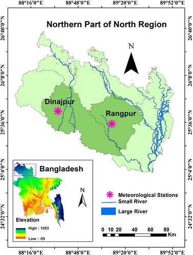
The physiographic of the study area is characterized by an alluvial plain and the slope is faces towards the south and southeast (Salam and Islam 2020). The study area is dominated by the Rangpur Saddle under the Indian platform in the sub-section of the Bengal basin, Bangladesh (Akhter et al. 2019). About 80% of the study area is composed of alluvial soil, while the rest of the area is composed of Barind clay. The study area is mostly dominated by agricultural land because of the presence of fertile soil (Salam et al. 2020). Approximately 80% of the areas are composed of recent alluvial soil and the rest of Barind clay. The deposit to groundwater by precipitation and flooding during the rainy season may affect the outcome of the increase in groundwater level. After a rainy season, part of the water rejuvenated into groundwater becomes discharged into the river channels, streams and low-lying regions (Jahan et al. 2010). Aquifer in northern region of Bangladesh is characterized by single to multiple layered Plio-Pleistocene age (thickness 5–40 m) and in the study area where semi-impervious clay-silt aquitard of Dupitila Formation under Recent-Pleistocene period (thickness 3.0–47.5 m) is noticed (Jahan et al. 2010). The groundwater has mainly been extracted for domestic and agricultural purposes, and a little amount is used for drinking uses (Islam et al. 2017). The utilization of groundwater in the study area is much higher in comparison with the rest of the country due to the scarcity of surface water resources and the key irrigated agricultural hub of the country. In several portions of the region, farmers have been enforced to replace their suction mode pumps with submersible pumps because of the steady decline in groundwater levels due to overuse of groundwater (Salam et al. 2020).

3. Methods

In this study, the ELM has been chosen as the main Machine Learning (ML) model embedded with several metaheuristic optimization algorithms. The ELM method has been proven to be not only a fast and efficient type of ANNs but capable of handling complicated hydrological problems (Alizamir et al. 2018). Also, several studies claimed that integrating metaheuristic algorithms with the ELM empowers its performance in simulating and predicting complex phenomena (Wu et al. 2020; Yang et al. 2021). Having a general and proper evaluation for the application of various integrative models, three different classes of metaheuristic algorithm have been selected and embedded with the ELM, as below:

• The first class of algorithms includes the Genetic Algorithm (GA) – developed in the 1980s for engineering applications (Goldberg and Samtani 1986) – and the Particle Swarm Optimization (PSO) – introduced in 1995 (Eberhart and Kennedy 1995) – which are two well-known traditional optimization techniques. Since their abilities and efficiencies have been tested and appraised in several studies (Mahdavi-Meymand et al. 2021; Fadaee et al. 2022), applying these algorithms can provide a good platform for the evaluation of the other techniques applied in this study.

• The second class involves two recently developed algorithms namely the Grey Wolf Optimization (GWO) – introduced in 2014 (Mirjalili et al. 2014) – and Whale Optimization Algorithm (WOA) – introduced in 2016 (Mirjalili and Lewis 2016). Some up-to-date researchers have already assessed the potential performance of these algorithms in hydrology with positive outcomes (Tikhamarine et al. 2020; Adnan et al. 2021).

• The third class consists of two newly introduced algorithms viz. the Harris Hawks Optimizer (HHO) – introduced in 2019 (Heidari et al. 2019) – and the Jellyfish Search Optimizer (JSO) – introduced in 2021 (Chou and Truong 2021). Since the performance and effectiveness of these novel methods have not been thoroughly assessed in modelling groundwater, thus, comparing the outcomes of these algorithms with the other two classes (GA, PSO, GWO, & WOA) gives a general appraisal of their optimization capability integrated with the ELM method.

In the following, brief descriptions of the logistics and methodology behind the ELM model along with the applied metaheuristic algorithms are given.

3.1. Extreme learning machine (ELM)

Since their development, FeedForward Neural Networks (FFNN), have been reported as capable and effective universal approximators for mapping the nonlinear nature of complex hydrological phenomena (Huang et al. 2006a; Zounemat-Kermani et al. 2021b). However, FFNNs face a shortcoming of being slow and having high computational time in dealing with high-dimensional complicated problems. This issue originated from two features of the FFNNs’ learning procedure including (i) the gradient-based learning algorithms and (ii) the iterative procedure for adjusting the networks’ parameters. Due to these inefficiencies of the FFNN, Huang et al. (2004) introduced a faster and more efficient version of the single-layer FFNN (SLFN) called the Extreme Learning Machine (ELM).

Assuming an SLFN. the main function for mapping the n numbers of the training input data, $\mathrm{x}=[x_1,x_2,\dots ,x_n],$ and N number of neurons in the hidden layer into the output value (target) can be written as below (1) $$f(x)=\sum _{j=1}^n\sum _{i=1}^N{\mathrm{\beta }}_{i}g(w_i{x}_j+b_i)$$(1) where $w_i=[w_{i1},w_{i2},\dots ,w_{in]}$ stand for the input weight vector that links the input layer to the hidden layer. ${\mathrm{\beta }}_i=[{\beta }_i,{\beta }_2,\dots ,{\beta }_N]$ represents the output weight vector that links the hidden nodes to output nodes. 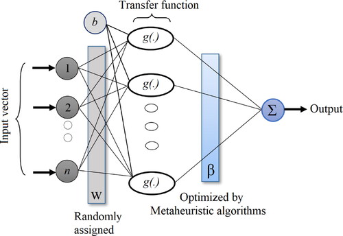$b$ is the hidden layer bias vector. g(.) is known as the transfer or activation function for calculating the hidden neuron output. In the ELM, the sigmoid and Gaussian functions are the most commonly used transfer functions that can be written as below: (2) $$g(x_i)=h(x_i)=\frac{e^{x_i}}{1+e^{x_i}}$$(2) (3) $$g(x_i)=h(a,c,x_i)=\hspace{0.17em}\exp \hspace{0.17em}(-a{\Vert \Vert x_i-c\Vert \Vert }^2)$$(3)

In relation (3) a and c denote the variables for the Gaussian transfer function. Figure 2 illustrates the schematic design for the ELM model. Although the ELM and FFNN follow the same structure, they have different training processes. In the ELM, unlike in the FFNN, all the network’s parameters, the input weight matrix (w), and hidden layer biases (b) do not have to be tuned during the iterative training process. Instead, w and b are initially allocated with some random variables. During the iterative training process, the ELM focuses on optimizing the output weight vector ($\mathrm{\beta }$) so that the network’s error is minimized, ideally ${\sum }_{i=1}^N\Vert \Vert y_i-t_i\Vert \Vert =0$ (y is the output of the model and t is the target value). If we assume H as the randomized hidden layer output matrix, and T as the target matrix, N system of equations are formed as below: (4) $$\mathbf{H}\mathrm{\beta }=\mathbf{T}$$(4) where (5) $$\mathbf{H}=\left[\begin{array}{cccc}g(x_{11})& g(x_{12})& \dots & g(x_{1N})\\ :& :& \dots & :\\ :& :& \dots & :\\ g(x_{n1})& g(x_{n2})& \dots & g(x_{nN})\end{array}\right]\mathbf{T}=\left[\begin{array}{c}{t}_1^T\\ :\\ :\\ t_n^T\end{array}\right]$$(5)

Figure 2. The general schematic structure of the ELM model.

One can write $\mathrm{\beta }={\mathbf{H}}^{+}\mathbf{T}$ as a system of linear equation for calculating the output weights ${\mathbf{H}}^{+}$ is known as the Moore–Penrose generalized inverse of the $\mathrm{\beta }$ matrix. This system of equation can be solved using least-square methods (Huang et al. 2006a; Zounemat-Kermani et al. 2021a).

3.2. Optimization algorithms

3.2.1. Genetic algorithm (GA)

The genetic algorithm (GA) is a well-known evolutionary algorithm inspired by the natural selection of species in the environment (Mitchell 1996). The GA has been proven to generate proper and high-quality solutions to either simple or complicated optimization problems. This algorithm uses three main operators namely selection, mutation, and crossover during the optimization process. Initially, a random population is created based on the features of the problem. Each individual in the population has its own chromosome that represents a possible solution to the problem. The merit of each solution is evaluated according to its fitness values. According to the calculated fitness of each individual, the first population passes its traits to the next generation (offspring). On average, it is expected that the individuals of the next generation will show a better performance in reaching the final solution of the problem. The process of creating a new generation will be continued until reaching the desired solution.

3.2.2. Particle swarm optimization (PSO)

Undoubtedly, the PSO is one of the most well cited and known metaheuristic algorithms that has been employed in several optimization problems (Eberhart and Kennedy 1995).

This nature-inspired algorithm was developed based on the movement behaviour of fish schools and birds’ flocks in the nature. Similar to the GA, some randomly generated individuals (agents or particles) are generated. Each particle takes part in a swarm through the solution space, and moves toward the best solution based on its own movement as well as the swarm movement. During the iterative procedure, the location and speed of the particles are adjusted according to the calculated fitness value of the personal best (pbest) and swarm/global best (gbest). Considering these two values, leads the algorithm to the best agent.

3.2.3. Grey wolf optimization algorithm (GWO)

The GWO, which has gained a lot of attention recently, was proposed by Mirjalili et al. (2014). Simply, the algorithm simulates the hunting behaviour of grey wolves in a pack. The pack hunts according to a leadership skill and social hierarchy of agents. In a pack, four main types of agents can be distinguished: (i) alpha, (ii) beta, (iii) delta, and (iv) omega. Alpha wolves are decision-makers that organize and lead the pack toward their aim. Beta wolves come second to the alpha wolves and reinforce the alphas’ decisions. They are also potential substitutes to the alpha wolves in case of death or disability. Omega and delta wolves act as subordinate members of the pack. Assumed the hunting process in GWO as searching for the best solution in an optimization problem, there are three main steps that should be applied: (i) tracking and approaching the prey, (ii) pursuing and stopping it from any further movement by encircling it, and (iii) attacking and hunting the prey.

3.2.4. Whale optimization algorithm, (WHO)

The WHO is a recent nature-based optimization algorithm (Mirjalili and Lewis 2016). Similar to the other population-based algorithms, at first, several random solutions based on some searching agents (candidate solutions) form the initial population. Like the GWO, in the WHO the hunters (humpback whales) try to find and hunt the prey. However, the searching and attacking processes are different in comparison to the pack hunting behaviours of grey wolves. Here, a so-called bubble-net feeding behaviour applies for searching the response space and finding the optimum solution. In this process, a humpback whale makes a trap by circling in a spiral path around prey while creating bubbles along with the spiral movement. After determining the initial random solutions and starting the optimization process, the positions of the search agents are updated based on the best search agent or a randomly selected agent. During the optimization process, three phases of (i) encircling, (ii) exploitation (bubble-net attacking), (iii) exploration (searching for prey), and (iv) hunting the prey are applied.

3.2.5. Harris hawks optimizer (HHO)

The HHO algorithm, like the PSO and WOA, is a nature-based swarm optimization algorithm based on Heidari et al. (2019). The HHO was inspired by the cooperative behaviour of Harris’ hawks chasing style for hunting prey using the surprise pounce strategy. In the surprise pounce strategy, several hawks attempt to attack and capture the prey cooperatively from different locations and in different directions. One of the hawks plays the role of a leader; however, its place can be taken by another party member when it loses the prey. The switching process finishes by confusing the prey and making it vulnerable in its defensive and escaping capabilities. After determining the initial search agents (population), the HHO starts its searching process for the best solution (hunting the prey) using the following phases: (i) exploration phase: exploring various areas to find the location of the prey, (ii) transition from exploration to exploitation, and (iii) exploitation phase and hunting the prey (Zhang et al. 2021).

3.2.6. Jellyfish search optimizer (JFO)

Proposed by Chou and Truong (2021), the JFO is a new swarm-based algorithm based on the behaviour of jellyfish for searching for food in the ocean. In their exploration for food, the jellyfish follow the ocean currents inside a jellyfish swarm using active and passive motions. They use a time control mechanism for adapting their movement inside the swarm, which moves along an ocean current. In the JFO algorithm, at first, a random population of jellyfish is produced. Nevertheless, to improve the diversity of the initial population, chaotic and logistic maps might be considered. Afterward, the two main phases of the JFO including (i) exploration and (ii) exploitation are developed. In the exploration phase, the swarm moves toward an ocean current, while in the exploitation phase each jellyfish moves inside the swarm for capturing food. The transmission strategy between these two phases is done by using the time control mechanism.

3.3. Integration process

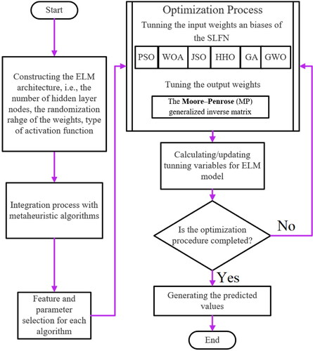
The integration procedure of the mentioned heuristic optimization algorithms (GA, PSO, GWO, WOA, HHO, & JFO) with the ELM employed in this paper can be defined as follows.

1. After constructing the ELM model, the optimization algorithms are employed to tune the input weights (w, see Eq. (1)(1) $$f(x)=\sum _{j=1}^n\sum _{i=1}^N{\mathrm{\beta }}_{i}g(w_i{x}_j+b_i)$$(1) ) and hidden biases (b, see Eq. (1)(1) $$f(x)=\sum _{j=1}^n\sum _{i=1}^N{\mathrm{\beta }}_{i}g(w_i{x}_j+b_i)$$(1) ) of the SLFN. It should be noted that for each of the six integrated individual models (i.e. the ELM-PSO, ELM-GA, ELM-GWO, ELM, WOA, ELM-HHO, ELM-JFO) the related metaheuristic algorithm is used to adjust the weights and biases so that there is no interaction among the different metaheuristic algorithm for this matter.

2. In the second phase of the optimization process, the Moore–Penrose (MP) generalized inverse matrix is used to calculate the output weights ($\mathrm{\beta },$ see Eq. (4)(4) $$\mathbf{H}\mathrm{\beta }=\mathbf{T}$$(4) ) based on the training set.

Having a better understanding of the optimization process used in this research, the general optimization procedure of the integrative ELM models is illustrated in Figure 3 in terms of the flowchart.

Figure 3. Schematic representation of the six applied integrative ELM models in this study.

4. Results and discussion

The viability of hybrid ELM methods, ELM-PSO, ELM-GA, ELM-GWO, ELM-WOA, ELM-HHO and ELM-JFO, is investigated and compared with standalone ELM in groundwater level (GWL) estimation using precipitation, temperature and previous GWL data as inputs. Daily data obtained from two stations, Bangladesh, were used in the applications. The models were validated with respect to the following comparison criteria: (6) $$\mathit{RMSE}:\mathit{Root}\mathrm{ }\mathit{Mean}\mathrm{ }\mathit{Square}\mathrm{ }\mathit{Error}=\frac{1}{N}{\sum }_{i=1}^N{\left[({\mathit{GWL}}_0{)}_i-({\mathit{GWL}}_C{)}_i\right]}^2$$(6) (7) $$\mathit{MAE}:\mathit{Mean}\mathrm{ }\mathit{Absolute}\mathrm{ }\mathit{Error}=\frac{1}{N}{\sum }_{i=1}^N\left|\right({\mathit{GWL}}_0{)}_i-\left({\mathit{GWL}}_C{)}_i\right|$$(7) (8) $$R^2:\mathit{Determination}\mathrm{ }\mathit{Coefficient}={\left[\frac{{\sum }_{t=1}^N\left({\mathit{GWL}}_o-\overline{{\mathit{GWL}}_o}\right)\left({\mathit{GWL}}_c-\overline{{\mathit{GWL}}_c}\right)}{\sqrt{{\sum }_{t=1}^N({\mathit{GWL}}_o-\overline{{\mathit{GWL}}_o}{)}^2({\mathit{GWL}}_c-\overline{{\mathit{GWL}}_c}{)}^2}}\right]}^2$$(8) (9) $$\mathit{NSE}:\mathit{Nash}-\mathit{Suutcliffe}=1-\frac{{\sum }_{i=1}^N\left[\right({\mathit{GWL}}_0{)}_i-({\mathit{GWL}}_c{)}_i{]}^2}{{\sum }_{i=1}^N\left[\right({\mathit{GWL}}_0{)}_i-{\overline{\mathit{GWL}}}_0{]}^2},-\mathrm{\infty }<\mathit{NSE}\le 1$$(9)

Where ${\mathit{GWL}}_c$ is computed GWL, ${\mathit{GWL}}_o$ is observed GWL, ${\overline{\mathit{GWL}}}_o$ is the mean of the observed GWL and, $N$ is data number. Table 1 gives the control parameter values of the implemented methods. Data were divided using 80% for training and −20% for testing and different values for control parameters were tried for the applied methods/algorithms. As clearly seen from Table 1, population and iteration were set to 40 and 10 for all algorithms and each algorithm was run 20 times and its mean accuracy was considered. First, precipitation, temperature and GWL data were separately used as inputs to the implemented models in estimating GWL. The combinations of optimum precipitation, optimum temperature and optimum GWL were considered in the models’ input.

Table 1. Parameter setting of the models and optimization algorithms used in the study.

Models/Algorithms	Parameters	Ranges/settings
ELM	Number of hidden neurons	$2\times F+1$ where $F$ is the number input features in the dataset
	Activation function	sigmoid
PSO	Cognitive component ($c_1$)	2
	Social component ($c_2$)	2
	inertia weight	0.2-0.9
GA	Crossover percentage	0.9
	Mutation percentage	0.5
	Mutation rate	0.1
GWO	$a$	decreased from 2 to 0
HHO	$\beta$	1.5
	$E_0$	$\in \left[-1, -1\right]$
JFO	–	–
WOA	$a$	$\in \left[0, 2\right]$
	$a2$	$\in \left[-1, -2\right]$
All algorithms	Population	40
	Number of iterations	150
	Number of runs for each Algorithm	20

Table 2 sums up the training and testing outcomes of the ELM-based models with precipitation (P) inputs in GWL estimation for the first station. Lags of the inputs were decided by taking into account the correlation analysis (e.g. partial autocorrelation function). In Table 2, PSO shows an ELM model tuned with PSO and vice versa. It is observed from the table that the RMSE, MAE, R² and NSE of the ELM-based models with Pt, Pt-1 inputs range 0.407–0.430, 0.312–0.341, 0.546–0.603 and 0.523–0.574 in the test period, respectively. Similarly, ranges of the RMSE, MAE, R² and NSE are 0.383–0.448, 0.296–0.338, 0.554–0.643 and 0.483–0.622 for inputs of Pt, Pt-1 and Pt-11 and they are 0.371–0.415, 0.293–0.321, 0.562–0.645 and 0.557–0.625 for the last input combination (Pt, Pt-1, Pt-11 and Pt-12) in the test stage, respectively. As evident from the ranges of the comparison statistics, the ELM-based models provide the best accuracy for the last input combination. Among the ELM-based methods, the ELM-JFO outperforms the others with the lowest RMSE (0.371 m), MAE (0.293 m) and the highest R² (0.645), NSE (0.625) in estimating GWL using only P inputs. It is also clear that combining metaheuristic algorithms with ELM improves the estimation accuracy.

Table 2. The comparison of different ELM precipitation based models in GWL estimation for the test period – Station 1.

Input combinations	Models	Training				Testing
		RMSE	MAE	R^2	NSE	RMSE	MAE	R^2	NSE
Pt,Pt-1	ELM	0.479	0.344	0.522	0.521	0.430	0.341	0.546	0.523
	PSO	0.418	0.306	0.660	0.660	0.417	0.328	0.572	0.551
	GA	0.411	0.302	0.670	0.670	0.411	0.325	0.586	0.565
	GWO	0.380	0.279	0.713	0.713	0.409	0.322	0.590	0.565
	WOA	0.365	0.269	0.740	0.740	0.407	0.319	0.600	0.572
	HHO	0.364	0.264	0.741	0.741	0.408	0.318	0.598	0.571
	JFO	0.363	0.265	0.742	0.742	0.407	0.312	0.603	0.574
	Mean	0.397	0.290	0.684	0.684	0.413	0.324	0.585	0.560
Pt,Pt-1,Pt-11	ELM	0.441	0.327	0.627	0.593	0.448	0.338	0.554	0.483
	PSO	0.418	0.306	0.660	0.660	0.417	0.328	0.573	0.552
	GA	0.416	0.304	0.662	0.662	0.417	0.327	0.574	0.552
	GWO	0.377	0.276	0.720	0.720	0.402	0.313	0.606	0.582
	WOA	0.362	0.266	0.745	0.745	0.406	0.308	0.610	0.575
	HHO	0.353	0.257	0.757	0.757	0.385	0.305	0.635	0.619
	JFO	0.352	0.253	0.759	0.759	0.383	0.296	0.643	0.622
	Mean	0.388	0.284	0.704	0.699	0.408	0.316	0.599	0.569
Pt,Pt-1,Pt-11,Pt-12	ELM	0.432	0.326	0.615	0.610	0.415	0.321	0.562	0.557
	PSO	0.406	0.296	0.679	0.679	0.410	0.323	0.589	0.567
	GA	0.402	0.291	0.684	0.684	0.410	0.322	0.593	0.566
	GWO	0.363	0.266	0.741	0.741	0.398	0.304	0.616	0.583
	WOA	0.351	0.257	0.760	0.760	0.403	0.306	0.612	0.580
	HHO	0.333	0.244	0.784	0.784	0.377	0.302	0.642	0.624
	JFO	0.344	0.250	0.770	0.770	0.371	0.293	0.645	0.625
	Mean	0.376	0.276	0.719	0.718	0.398	0.310	0.609	0.586

Training and testing outcomes of the ELM-based models with temperature (T) inputs in GWL estimation are reported in Table 3 for the 1st station. Here also the models with the last input combination comprising inputs of Tt, Tt-1, Tt-11 and Tt-12 generally provides better GWL estimates in the test stage compared to other two input combinations. This can be understood by comparing ranges of the RMSE, MAE, R² and NSE statistics or mean statistics indicated by the bold values. Hybrid ELM models performed superior to the standalone ELM in GWL estimation and the ELM-JFO produced the best accuracy with the lowest RMSE (0.427 m), MAE (0.336 m) and the highest R² (0.546), NSE (0.533) in the test phase. Compared to ELM-based models with precipitation inputs given in Table 2, the ELM models with temperature inputs generally give worse estimates and this reveals that P has more influence on GWL than the T in this station.

Table 3. The comparison of different ELM temperature based models in GWL estimation for the test period – Station 1.

Input combinations	Models	Training				Testing
		RMSE (m^3/s)	MAE (m^3/s)	R^2	NSE	RMSE (m^3/s)	MAE (m^3/s)	R^2	NSE
Tt,Tt-1	ELM	0.560	0.433	0.426	0.420	0.496	0.396	0.423	0.406
	PSO	0.539	0.422	0.431	0.431	0.476	0.384	0.433	0.416
	GA	0.526	0.406	0.462	0.460	0.464	0.371	0.466	0.446
	GWO	0.461	0.344	0.580	0.580	0.456	0.354	0.507	0.463
	WOA	0.442	0.327	0.632	0.631	0.455	0.345	0.524	0.496
	HHO	0.430	0.314	0.646	0.646	0.438	0.331	0.545	0.506
	JFO	0.421	0.306	0.655	0.655	0.430	0.328	0.557	0.524
	Mean	0.483	0.365	0.547	0.546	0.459	0.358	0.494	0.465
Tt,Tt-1,Tt-11	ELM	0.556	0.425	0.430	0.430	0.482	0.387	0.433	0.421
	PSO	0.536	0.414	0.440	0.440	0.472	0.377	0.443	0.429
	GA	0.539	0.419	0.439	0.439	0.474	0.378	0.441	0.426
	GWO	0.444	0.327	0.607	0.607	0.439	0.338	0.531	0.501
	WOA	0.418	0.297	0.651	0.651	0.440	0.332	0.545	0.524
	HHO	0.398	0.284	0.691	0.691	0.424	0.321	0.578	0.537
	JFO	0.395	0.280	0.695	0.695	0.417	0.316	0.585	0.552
	Mean	0.469	0.349	0.565	0.565	0.450	0.350	0.508	0.484
Tt,Tt-1,Tt-11,Tt-12	ELM	0.536	0.414	0.440	0.440	0.475	0.380	0.447	0.438
	PSO	0.531	0.411	0.449	0.449	0.462	0.366	0.529	0.517
	GA	0.526	0.408	0.465	0.461	0.448	0.342	0.532	0.528
	GWO	0.463	0.327	0.603	0.603	0.434	0.331	0.549	0.543
	WOA	0.444	0.313	0.615	0.615	0.424	0.324	0.576	0.556
	HHO	0.402	0.285	0.678	0.678	0.413	0.305	0.591	0.569
	JFO	0.393	0.276	0.698	0.698	0.405	0.301	0.599	0.577
	Mean	0.471	0.348	0.564	0.564	0.437	0.336	0.546	0.533

Table 4 presents the RMSE, MAE, R² and NSE statistics of the ELM-based models with the previous GWL inputs in estimating GWL of the 1st station. As seen from the table, 1st input combination produced mean RMSE, MAE, R² and NSE as 0.340 m, 0.226 m, 0.680 and 0.651 in the test stage while the corresponding values are 0.268 m, 0.153 m, 0.802 and 0.778 for the 2nd input combination and 0.242 m, 0.126 m, 0.835 and 0.815 for the 3rd (last) input combination, respectively. It is clear that hybridization of ELM with metaheuristic algorithms considerably improves the its accuracy and the JFO provides the best improvement; decreases in RMSE and MAE of standalone ELM from 0.283 m to 0.211 m and from 0.154 m to 0.106 m and increases in R² and NSE from 0.806 to 0.859 and from 0.773 to 0.857 in the test stage. Considering GWL inputs performs much better accuracy than the precipitation and temperature inputs. For example, in case of last input combination, mean RMSE, MAE, R² and NSE of P-based models were improved by 39%, 59%, 37% and 39%, respectively. The main reason of this might be the high autocorrelation in the daily GWL data.

Table 4. The comparison of different ELM groundwater level based models in GWL estimation for the test period – Station 1.

Input combinations	Models	Training				Testing
		RMSE (m^3/s)	MAE (m^3/s)	R^2	NSE	RMSE (m^3/s)	MAE (m^3/s)	R^2	NSE
GWLt-1,GWLt-2	ELM	0.369	0.215	0.617	0.617	0.397	0.254	0.589	0.533
	PSO	0.344	0.198	0.660	0.660	0.375	0.247	0.650	0.592
	GA	0.331	0.190	0.618	0.618	0.397	0.252	0.666	0.622
	GWO	0.288	0.166	0.798	0.798	0.332	0.225	0.686	0.656
	WOA	0.248	0.146	0.863	0.863	0.303	0.212	0.707	0.701
	HHO	0.242	0.134	0.872	0.872	0.292	0.202	0.728	0.723
	JFO	0.232	0.124	0.885	0.885	0.283	0.194	0.738	0.732
	Mean	0.293	0.167	0.759	0.759	0.340	0.226	0.680	0.651
GWLt-1,GWLt-2,GWLt-11	ELM	0.280	0.163	0.755	0.755	0.321	0.173	0.765	0.728
	PSO	0.274	0.153	0.782	0.775	0.308	0.181	0.781	0.740
	GA	0.262	0.144	0.787	0.781	0.305	0.169	0.786	0.744
	GWO	0.233	0.120	0.881	0.878	0.249	0.145	0.805	0.785
	WOA	0.210	0.099	0.904	0.904	0.244	0.141	0.816	0.795
	HHO	0.199	0.090	0.926	0.926	0.231	0.138	0.828	0.818
	JFO	0.191	0.088	0.934	0.934	0.222	0.128	0.834	0.833
	Mean	0.236	0.122	0.853	0.850	0.268	0.153	0.802	0.778
GWLt-1,GWLt-2,GWLt-11,GWLt-12	ELM	0.256	0.146	0.846	0.844	0.283	0.154	0.806	0.773
	PSO	0.252	0.141	0.849	0.849	0.266	0.143	0.816	0.780
	GA	0.244	0.120	0.858	0.858	0.252	0.133	0.829	0.794
	GWO	0.208	0.099	0.914	0.914	0.238	0.119	0.837	0.805
	WOA	0.191	0.085	0.946	0.946	0.226	0.115	0.846	0.842
	HHO	0.175	0.072	0.952	0.952	0.218	0.110	0.853	0.851
	JFO	0.168	0.065	0.968	0.968	0.211	0.106	0.859	0.857
	Mean	0.213	0.104	0.905	0.904	0.242	0.126	0.835	0.815

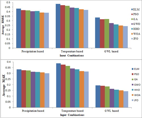
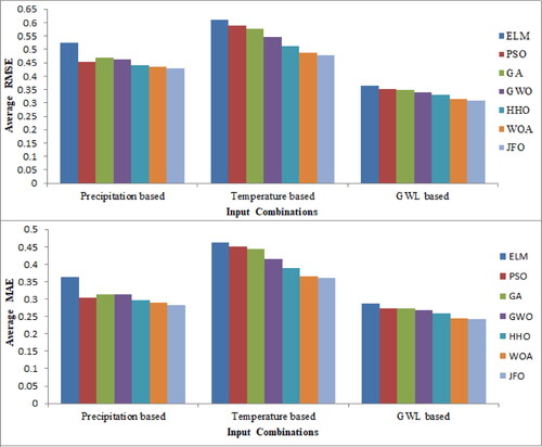
Figure 4 compares the best ELM-based models for the test stage using time variation graphs. It is evident from the figure (especially from the zoomed graphs) that the ELM-JFO follows the corresponding observed values closer compared to other models and the single ELM model cannot catch the extreme GWL well. Figure 5 illustrates scatterplots of the observed and predicted GWL by different hybrid ELM models for the test period of the best input combination. It is visible from the scatterplots that the JFO produces the least scattered predictions followed by the WOA, HHO and GWO, respectively. Figure 6 compares the ELM based models on a Taylor diagram. It is clear from the graph that the JFO has the highest correlation and the least RMSE among the considered algorithms. The average RMSE and MAE of the models’ predictions for all input combinations are illustrated in Figure 7. It is clearly observed from the figure that the JFO has the least average RMSE and MAE for all input cases and it is followed by the WOA, HHO and GWO as also observed from the scatterplots, respectively. Furthermore, it is seen from Figure 7 that the precipitation is more affective on GWL than the air temperature.

Figure 4. Time variation graphs of the observed and predicted GWL by different ELM based models in the test period using best input combination – Station 1.

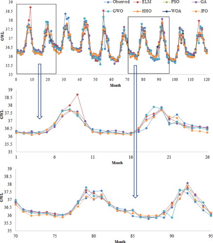
Figure 5. Scatterplots of the observed and predicted GWL by different ELM based models in the test period using best input combination – Station 1.

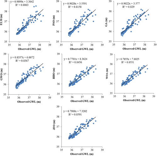
Figure 6. Taylor diagrams of the predicted GWL by different ELM based models in the test period using best input combination – Station 1.

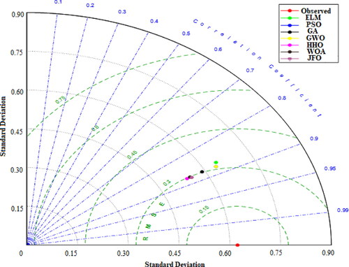
Figure 7. Average RMSE and MAE of the applied models in predicting GWL using all input combinations during test period – Station 1.

Training and testing outcomes of the ELM-based models with P, T and GWL inputs are provided in Tables 5–7 for the 2nd station, respectively. In this station also last input combination generally gave the best GWL estimation accuracy. It is apparent that P-based models perform better than T-based models but they provide worse accuracy compared to GWL-based models. Using GWL as input improves the accuracy of P-based ELM models by 33%, 24%, 52% and 52% with respect to mean RMSE, MAE, R² and NSE in the testing stage of the last input combination, respectively. The accuracy of standalone ELM model is improved by using metaheuristic algorithms in all input cases (e.g. P, T and GWL) and among them, the JFO gets the first rank. The ELM-JFO improved the RMSE, MAE, R² and NSE of standalone ELM by 9%, 16%, 18% and 18% for P inputs, by 11%, 12%, 13% and 13% for T inputs and by 9%, 9%, 2% and 2% for GWL inputs in the testing phase of the last input combination, respectively.

Table 5. The comparison of different ELM precipitation based models in GWL estimation for the test period – Station 2.

Input combinations	Models	Training				Testing
		RMSE	MAE	R^2	NSE	RMSE	MAE	R^2	NSE
Pt,Pt-1	ELM	0.501	0.358	0.609	0.609	0.569	0.389	0.465	0.460
	PSO	0.448	0.336	0.755	0.755	0.426	0.276	0.540	0.537
	GA	0.446	0.325	0.757	0.757	0.471	0.318	0.540	0.534
	GWO	0.436	0.308	0.792	0.792	0.488	0.349	0.559	0.555
	WOA	0.395	0.279	0.787	0.787	0.450	0.315	0.607	0.601
	HHO	0.395	0.278	0.803	0.803	0.443	0.312	0.611	0.606
	JFO	0.393	0.275	0.807	0.807	0.440	0.305	0.613	0.611
	Mean	0.430	0.308	0.758	0.758	0.470	0.323	0.562	0.558
Pt,Pt-1,Pt-11	ELM	0.439	0.319	0.734	0.734	0.518	0.343	0.496	0.492
	PSO	0.435	0.318	0.746	0.746	0.476	0.323	0.557	0.553
	GA	0.435	0.313	0.753	0.753	0.475	0.323	0.556	0.550
	GWO	0.434	0.313	0.798	0.798	0.456	0.301	0.587	0.581
	WOA	0.378	0.266	0.794	0.794	0.446	0.294	0.632	0.631
	HHO	0.375	0.260	0.817	0.817	0.437	0.282	0.637	0.634
	JFO	0.367	0.253	0.828	0.828	0.431	0.276	0.643	0.640
	Mean	0.409	0.292	0.781	0.781	0.463	0.306	0.587	0.583
Pt,Pt-1,Pt-11,Pt-12	ELM	0.402	0.262	0.752	0.752	0.491	0.356	0.513	0.510
	PSO	0.330	0.214	0.719	0.719	0.462	0.310	0.563	0.561
	GA	0.318	0.202	0.747	0.747	0.457	0.301	0.580	0.576
	GWO	0.298	0.195	0.771	0.771	0.442	0.289	0.616	0.612
	WOA	0.285	0.177	0.802	0.802	0.428	0.283	0.643	0.641
	HHO	0.283	0.170	0.794	0.794	0.421	0.278	0.656	0.653
	JFO	0.272	0.159	0.802	0.802	0.418	0.270	0.660	0.656
	Mean	0.313	0.197	0.770	0.770	0.446	0.298	0.604	0.601

Table 6. The comparison of different ELM temperature based models in GWL estimation for the test period – Station 2.

Input combinations	Models	Training				Testing
		RMSE (m^3/s)	MAE (m^3/s)	R^2	NSE	RMSE (m^3/s)	MAE (m^3/s)	R^2	NSE
Tt,Tt-1	ELM	0.532	0.377	0.715	0.715	0.630	0.493	0.515	0.511
	PSO	0.494	0.357	0.728	0.728	0.598	0.476	0.524	0.521
	GA	0.490	0.354	0.731	0.731	0.596	0.474	0.525	0.513
	GWO	0.463	0.343	0.740	0.740	0.579	0.440	0.546	0.542
	WOA	0.430	0.319	0.757	0.757	0.560	0.432	0.563	0.560
	HHO	0.394	0.287	0.848	0.848	0.522	0.422	0.611	0.606
	JFO	0.390	0.285	0.851	0.851	0.520	0.420	0.615	0.613
	Mean	0.456	0.332	0.767	0.767	0.572	0.451	0.557	0.552
Tt,Tt-1,Tt-11	ELM	0.455	0.332	0.739	0.739	0.602	0.451	0.528	0.523
	PSO	0.447	0.320	0.764	0.764	0.586	0.434	0.545	0.539
	GA	0.442	0.310	0.788	0.788	0.566	0.425	0.550	0.542
	GWO	0.403	0.291	0.818	0.818	0.509	0.391	0.599	0.591
	WOA	0.351	0.255	0.821	0.821	0.492	0.381	0.666	0.661
	HHO	0.344	0.241	0.839	0.839	0.466	0.343	0.674	0.670
	JFO	0.324	0.213	0.853	0.853	0.461	0.337	0.698	0.695
	Mean	0.395	0.280	0.803	0.803	0.526	0.395	0.608	0.603
Tt,Tt-1,Tt-11,Tt-12	ELM	0.445	0.331	0.749	0.749	0.597	0.443	0.533	0.527
	PSO	0.434	0.329	0.759	0.759	0.580	0.440	0.539	0.529
	GA	0.428	0.316	0.768	0.768	0.571	0.432	0.547	0.542
	GWO	0.410	0.303	0.783	0.783	0.548	0.416	0.577	0.563
	WOA	0.364	0.257	0.818	0.818	0.486	0.352	0.659	0.655
	HHO	0.360	0.252	0.828	0.828	0.473	0.334	0.665	0.658
	JFO	0.330	0.230	0.846	0.846	0.457	0.324	0.701	0.694
	Mean	0.396	0.288	0.793	0.793	0.530	0.392	0.603	0.595

Table 7. The comparison of different ELM groundwater level based models in GWL estimation for the test period – Station 2.

Input combinations	Models	Training				Testing
		RMSE (m^3/s)	MAE (m^3/s)	R^2	NSE	RMSE (m^3/s)	MAE (m^3/s)	R^2	NSE
GWLt-1,GWLt-2	ELM	0.326	0.243	0.883	0.883	0.426	0.349	0.875	0.870
	PSO	0.315	0.232	0.891	0.891	0.421	0.348	0.876	0.865
	GA	0.314	0.232	0.892	0.892	0.413	0.344	0.874	0.870
	GWO	0.305	0.223	0.898	0.898	0.405	0.341	0.880	0.869
	WOA	0.293	0.218	0.903	0.903	0.403	0.324	0.888	0.885
	HHO	0.289	0.213	0.906	0.906	0.400	0.322	0.893	0.887
	JFO	0.286	0.211	0.904	0.904	0.398	0.320	0.899	0.892
	Mean	0.304	0.225	0.897	0.897	0.409	0.336	0.884	0.877
GWLt-1,GWLt-2,GWLt-11	ELM	0.248	0.200	0.922	0.922	0.341	0.260	0.892	0.892
	PSO	0.226	0.180	0.944	0.944	0.323	0.240	0.903	0.902
	GA	0.221	0.177	0.948	0.948	0.318	0.236	0.908	0.905
	GWO	0.213	0.161	0.955	0.955	0.311	0.232	0.916	0.910
	WOA	0.201	0.156	0.962	0.962	0.291	0.227	0.923	0.921
	HHO	0.198	0.150	0.967	0.967	0.275	0.211	0.931	0.929
	JFO	0.193	0.147	0.969	0.969	0.271	0.209	0.935	0.933
	Mean	0.214	0.167	0.952	0.952	0.304	0.231	0.915	0.913
GWLt-1,GWLt-2,GWLt-11,GWLt-12	ELM	0.233	0.182	0.940	0.940	0.328	0.250	0.900	0.895
	PSO	0.223	0.171	0.945	0.945	0.311	0.232	0.910	0.906
	GA	0.221	0.170	0.948	0.948	0.313	0.239	0.909	0.902
	GWO	0.208	0.160	0.952	0.952	0.307	0.235	0.914	0.911
	WOA	0.193	0.147	0.959	0.959	0.295	0.226	0.919	0.914
	HHO	0.190	0.145	0.961	0.961	0.269	0.203	0.933	0.930
	JFO	0.176	0.133	0.966	0.966	0.261	0.201	0.936	0.934
	Mean	0.206	0.158	0.953	0.953	0.298	0.227	0.917	0.913

Table 8 reports the comparison statistics of the ELM-based models with various combinations of optimal P, T and GWL inputs for the 1st station. The OPT P, OPT T and OPT GWL in the table indicate the optimal precipitation, optimal temperature and optimal GWL inputs. The OPT P was decided considering the P-based input combination which produced the least RMSE, MAE and the highest R² and NSE and vice versa. For example, OPT P, OPT T in Table 8 corresponds to combination of Pt, Pt-1, Pt-11, Pt-12 (from Table 2) and Tt, Tt-1, Tt-11, Tt-12 (from Table 3). It is clear from the mean statistics in Table 8 that combining optimal P and optimal T inputs (OPT P, OPT T) considerably improves the estimation accuracy of P- and T-based ELM models; decreases in RMSE and MAE of P-based models are from 0.398 m and 0.310 m to 0.351 m and 0.271 m and increases in R² and NSE are from 0.609 and 0.586 to 0.742 and 0.733 while for the T-based models, the RMSE and MAE decrease from 0.437 m and 0.366 m to 0.351 m and 0.271 m, the R² and NSE increase from 0.546 and 0.533 to 0.742 and 0.733. All hybrid ELM methods perform superior to the standalone ELM and the ELM-JFO presents the best accuracy with the lowest RMSE (0.318 m) and MAE (0.233 m) and the highest R² (0.773) and NSE (0.762). It should be noted that the input combination (OPT T, OPT P) is very useful in the places where GWL data are missing. In such a case, GWL-based models are not applicable in practice. It is also clear in Table 8 that the best estimates belong to the ELM-based models with optimal P, T and GWL inputs (OPT T, OPT P, OPT GWL). It improves the mean RMSE, MAE, R² and NSE of the GWL-based ELM models by 26%, 44%, 6% and 62% in the testing stage, respectively.

Table 8. The comparison of different ELM based models in GWL estimation for the test period using optimal input combinations – Station 1.

Optimal input combinations	Models	Training					Testing
		RMSE (m^3/s)	MAE (m^3/s)	R^2	NSE	RMSE (m^3/s)		MAE (m^3/s)	R^2	NSE
OPT P,OPT T	ELM	0.389	0.281	0.674	0.674	0.406		0.320	0.690	0.676
	PSO	0.352	0.258	0.731	0.730	0.365		0.289	0.726	0.718
	GA	0.355	0.249	0.738	0.726	0.360		0.284	0.733	0.730
	GWO	0.308	0.223	0.788	0.788	0.354		0.275	0.752	0.740
	WOA	0.291	0.212	0.811	0.811	0.334		0.256	0.756	0.749
	HHO	0.282	0.200	0.822	0.822	0.322		0.240	0.763	0.753
	JFO	0.274	0.196	0.831	0.831	0.318		0.233	0.773	0.762
	Mean	0.322	0.231	0.771	0.769	0.351		0.271	0.742	0.733
OPT P,OPT GWL	ELM	0.312	0.213	0.810	0.810	0.387		0.281	0.740	0.692
	PSO	0.245	0.181	0.883	0.883	0.314		0.241	0.776	0.752
	GA	0.240	0.174	0.886	0.885	0.309		0.238	0.779	0.777
	GWO	0.235	0.157	0.900	0.900	0.306		0.223	0.805	0.801
	WOA	0.229	0.148	0.907	0.907	0.304		0.220	0.814	0.812
	HHO	0.217	0.138	0.915	0.915	0.301		0.216	0.818	0.815
	JFO	0.197	0.128	0.924	0.924	0.292		0.210	0.823	0.820
	Mean	0.239	0.163	0.889	0.889	0.316		0.233	0.794	0.781
OPT T,OPT GWL	ELM	0.253	0.166	0.847	0.857	0.264		0.148	0.798	0.783
	PSO	0.227	0.154	0.858	0.858	0.245		0.155	0.817	0.814
	GA	0.223	0.145	0.858	0.858	0.245		0.154	0.817	0.815
	GWO	0.206	0.104	0.915	0.915	0.239		0.144	0.829	0.824
	WOA	0.189	0.085	0.937	0.937	0.234		0.133	0.838	0.830
	HHO	0.178	0.083	0.950	0.950	0.229		0.145	0.842	0.839
	JFO	0.147	0.066	0.981	0.981	0.226		0.139	0.846	0.844
	Mean	0.203	0.115	0.907	0.908	0.240		0.145	0.827	0.821
OPT P,OPT T,OPT GWL	ELM	0.230	0.134	0.862	0.862	0.258		0.134	0.823	0.793
	PSO	0.226	0.131	0.867	0.867	0.241		0.127	0.842	0.821
	GA	0.228	0.133	0.865	0.865	0.233		0.128	0.840	0.834
	GWO	0.173	0.091	0.923	0.923	0.233		0.139	0.842	0.833
	WOA	0.152	0.077	0.945	0.945	0.229		0.145	0.840	0.839
	HHO	0.140	0.067	0.956	0.956	0.227		0.123	0.853	0.843
	JFO	0.105	0.044	0.983	0.983	0.216		0.119	0.857	0.848
	Mean	0.179	0.097	0.914	0.914	0.234		0.131	0.842	0.830

Training and testing statistics of the ELM-based models with different combinations of optimum P, T and GWL inputs are compared in Table 9 for the second station. Here also the combination of optimal P and T inputs considerably improves the accuracy of P-based and T-based models in estimating GWL. The ELM models with optimal P and optimal T inputs respectively improve the mean RMSE, MAE, R² and NSE of the P-based ELM models by 21%, 9%, 23% and 22% while for the T-based models, the improvements are 34%, 31%, 23% and 23%, respectively. The comparison of Tables 7 and 9 clearly indicates that combining optimal T or optimal P with optimal GWL inputs improves the accuracy of GWL-based models in the second station; improvements in mean RMSE, MAE, R² and NSE of the GWL-based models are by 7.7%, 8.4%, 0.4% and 0.3% using optimal P and GWL inputs and by 4%, 6.2%, 0.8% and 0.9% using optimal T and GWL inputs, respectively. Combination of three optimal input variables (OPT T, OPT P, OPT GWL) provides the best accuracy among the alternative input combinations. By considering this input combination, mean RMSE and MAE of GWL-based models decrease from 0.298 m and 0.227 m to 0.277 m and 0.203 and R² and NSE increase from 0.917 and 0.913 to 0.930 and 0.925 in the testing stage. ELM-JFO has the best accuracy with the lowest RMSE (0.246 m), MAE (0.179 m) and the highest R² (0.948) and NSE (0.941) in estimating daily GWL. It improves the RMSE, MAE, R² and NSE of the standalone ELM model by 1.6%, 3.5%, 7.5% and 7.3% for the optimal P and optimal T inputs, by 23%, 21%, 4.3% and 3.9% for the optimal P and GWL inputs, by 14%, 10%, 2.8% and 2.8% for the optimal T and GWL inputs and by 13%, 11%, 2.4% and 2% for the optimal P, T and GWL inputs in the testing stage, respectively.

Table 9. The comparison of different ELM based models in GWL estimation for the test period using optimal input combinations – Station 2.

Optimal input combinations	Models	Training					Testing
		RMSE (m^3/s)	MAE (m^3/s)	R^2	NSE	RMSE (m^3/s)	MAE (m^3/s)	R^2	NSE
OPT P,OPT T	ELM	0.497	0.387	0.822	0.822	0.513	0.399	0.667	0.661
	PSO	0.480	0.376	0.773	0.773	0.527	0.396	0.690	0.683
	GA	0.450	0.340	0.789	0.789	0.525	0.407	0.727	0.719
	GWO	0.480	0.376	0.773	0.773	0.527	0.396	0.690	0.683
	WOA	0.444	0.336	0.822	0.822	0.514	0.386	0.735	0.727
	HHO	0.435	0.323	0.848	0.848	0.471	0.357	0.748	0.737
	JFO	0.432	0.316	0.854	0.854	0.454	0.352	0.759	0.757
	Mean	0.460	0.351	0.811	0.811	0.505	0.385	0.717	0.709
OPT P,OPT GWL	ELM	0.194	0.151	0.958	0.958	0.356	0.264	0.883	0.882
	PSO	0.162	0.124	0.971	0.971	0.288	0.212	0.903	0.901
	GA	0.163	0.125	0.969	0.969	0.291	0.215	0.900	0.898
	GWO	0.155	0.123	0.972	0.972	0.257	0.207	0.927	0.916
	WOA	0.150	0.112	0.975	0.975	0.250	0.190	0.942	0.934
	HHO	0.143	0.102	0.978	0.978	0.247	0.188	0.945	0.938
	JFO	0.140	0.100	0.983	0.983	0.237	0.180	0.949	0.944
	Mean	0.158	0.120	0.972	0.972	0.275	0.208	0.921	0.916
OPT T,OPT GWL	ELM	0.219	0.175	0.947	0.947	0.333	0.236	0.899	0.896
	PSO	0.210	0.167	0.954	0.954	0.305	0.230	0.916	0.914
	GA	0.214	0.169	0.950	0.950	0.310	0.233	0.909	0.907
	GWO	0.181	0.137	0.964	0.964	0.272	0.202	0.932	0.923
	WOA	0.168	0.126	0.969	0.969	0.265	0.200	0.935	0.930
	HHO	0.151	0.114	0.975	0.975	0.262	0.196	0.937	0.935
	JFO	0.148	0.112	0.977	0.977	0.256	0.194	0.944	0.939
	Mean	0.184	0.143	0.962	0.962	0.286	0.213	0.924	0.921
OPT P,OPT T,OPT GWL	ELM	0.202	0.169	0.952	0.952	0.320	0.229	0.908	0.907
	PSO	0.193	0.149	0.959	0.959	0.298	0.222	0.918	0.914
	GA	0.192	0.149	0.959	0.959	0.288	0.212	0.923	0.921
	GWO	0.165	0.124	0.970	0.970	0.274	0.201	0.930	0.926
	WOA	0.162	0.122	0.971	0.971	0.262	0.195	0.937	0.932
	HHO	0.137	0.100	0.979	0.979	0.251	0.181	0.944	0.936
	JFO	0.129	0.092	0.982	0.982	0.246	0.179	0.948	0.941
	Mean	0.169	0.129	0.967	0.967	0.277	0.203	0.930	0.925

Figure 8 illustrates observed and predicted GWLs by the best ELM-based models for the test stage in the form of time variation graphs. For this station also the ELM-JFO predictions generally better follow the trend of observed GWL values compared to the other models. Figure 9 compares scatterplots of the observed and predicted GWL by several hybrid ELM models for the best input combination in the test period. In this station, also JFO has the least scattered predictions and it is followed by the WOA, HHO and GWO. Taylor diagram illustrated in Figure 10 reveals that the JFO has the best algorithm in improving ELM accuracy in GWL modelling with respect to correlation, RMSE and standard deviation. Figure 11 compares the ELM-based models with respect to average RMSE and MAE in the testing stage for all input combinations. Like the previous station, the JFO has the least average RMSE and MAE for all input cases and it is followed by the WOA, HHO and GWO, respectively. The best predictions were obtained from GWL based inputs while the temperature-based inputs provided the worst predictions.

Figure 8. Time variation graphs of the observed and predicted GWL by different ELM based models in the test period using best input combination – Station 2.

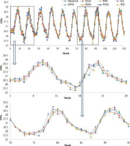
Figure 9. Scatterplots of the observed and predicted GWL by different ELM based models in the test period using best input combination – Station 2.

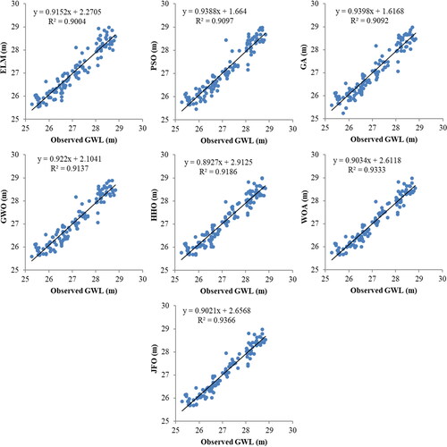
Figure 10. Taylor diagrams of the predicted GWL by different ELM based models in the test period using best input combination – Station 2.

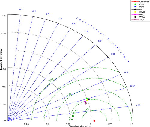
Figure 11. Average RMSE and MAE of the applied models in predicting GWL for all input combinations during test period – Station 2.

In the presented study, lagged precipitation, temperature and GWL data were first separately tried as inputs to the models so as to see the effect of these parameters on current GWL. This type of comparison is very essential especially for the basins where some GWL data are missing. In such cases, prediction of GWL using other effective input data such as precipitation and/or temperature is very practical. The developed models (improved ELM) can be successfully used for GWL prediction by the modellers and can provide useful information to decision makers or managers for planning and management of water resources. These types of models can be used as a module by integrating the hydrological analysis models.

Yoon et al. (2011) predicted GWL of two wells in a coastal aquifer by support vector machine (SVM) and artificial neural networks (ANN) using lagged GWL, precipitation (P) and tide levels (TL) as input to the models. They tried different input combinations (e.g. P + TL, GWL, P + G, TL + GWL and P + TL + GWL) and the best ANN and SVM models produced the NSE (R²) as 0.576 (0.768) and 0.582 (0.775) for one station and 0.534 (0.733) and 0.628 (0.793) for other station, respectively. Shakya et al. (2022) predicted GWL of Vidisha district in India using decision tree (DT), random forest (RF), ANN, SVM and neuro fuzzy (ANFIS) and they used rainfall, evapotranspiration and GWL as inputs. They obtained R² from the best DT, RF, SVM, ANN and ANFIS models as 0.88, 0.87, 0.86, 0.83 and 0.81, respectively. In the presented study, the ELM-JFO model produced R² and NSE of 0.842 and 0.830 for the first station and 0.930 and 0.925 for the second station, respectively which shows the accurateness of this model in GWL prediction.

5. Conclusions

The study investing acted the efficiency of hybrid ELM methods tuned with particle swarm optimization, grey wolf optimization, whale optimization algorithm, Harris Hawks optimizer and Jellyfish search optimizer in groundwater level estimation using daily precipitation, temperature and previous groundwater level data as inputs. Data were acquired from two stations of Bangladesh and methods were assessed based on RMSE, MAE, R² and NSE and some new graphical inspection methods. The following conclusions were reached after the applications:

• Comparing with the standalone ELM method, it was found that metaheuristic algorithms considerably improve the accuracy in the estimation of GWL.

• Comparison of the only precipitation and temperature inputs revealed that the precipitation has more influence on groundwater level compared to temperature.

• Adding GWL as inputs to ELM models provides much better accuracy than the precipitation and temperature inputs. This was expected because the daily GWL time series has strong autocorrelation.

• Among the all ELM methods, the ELM-JFO provided the best accuracy in daily GWL estimation using hydroclimatic inputs. The use of this method is recommended for accurate estimation of GWL and this information can be useful for related managers and planers to provide better water resources planning and management.

In the presented study, daily data of precipitation, air temperature and GWL for two locations were used to assess improved ELM based models. In future studies, more data (longer period and different intervals) from other locations can be used to more comprehensive evaluation of the proposed methods in GWL prediction. The proposed methods may be compared with other hybrid methods (e.g. SVM-based, ANFIS-based or ANN-based).

Author contributions

RMA and RRM designed the methodology and collected the datasets. RRM developed the models and applied the datasets. OK and HLD analyzed the results. ARMTI, OK, SM and MZM wrote the original manuscript. HLD and OK supervised the study. All the authors revised and improved the manuscript.

Acknowledgements

The authors would like to thank the pioneering researchers in fuzzy decision and other related fields. The authors would also like to express their sincere appreciation to the associate editor and the anonymous reviewers for their comments and suggestions.

Disclosure statement

No potential conflict of interest was reported by the authors.

Data availability statement

Data are available from the corresponding author on a reasonable request.

Additional information

Funding

This work was supported by the National Social Science Foundation of China (18BTJ029), Key Projects Of National Statistical Science Research Projects (2020LZ10), and Tertiary Education Scientific Research Project of Guangzhou Municipal Education Bureau (202235324). The APC was funded by the Postdoctoral Start-up Research Fund of Guangzhou University.

References

- Adnan RM, Mostafa R, Kisi O, Yaseen ZM, Shahid S, Zounemat-Kermani M. 2021. Improving streamflow prediction using a new hybrid ELM model combined with hybrid particle swarm optimization and grey wolf optimization. Knowledge-Based Syst. 230:107379.
- Agoubi B, Kharroubi A. 2019. Groundwater depth monitoring and short-term prediction: applied to El Hamma aquifer system, southeastern Tunisia. Arab J Geosci. 12(10):1–10.
- Akhavan-Amjadi M. 2020. Fetal electrocardiogram modelling using hybrid evolutionary firefly algorithm and extreme learning machine. Multidim Syst Sign Process. 31(1):117–133.
- Akhter S, Eibek KU, Islam S, Islam ARMT, Shen S, Chu R. 2019. Predicting spatiotemporal changes of channel morphology in the reach of Teesta River, Bangladesh using GIS and ARIMA modelling. Quat Int. 513:80–94.
- Alizadeh A, Rajabi A, Shabanlou S, Yaghoubi B, Yosefvand F. 2021. Modelling long-term rainfall-runoff time series through wavelet-weighted regularization extreme learning machine. Earth Sci Inform. 14(2):1047–1063.
- Alizamir M, Kisi O, Zounemat-Kermani M. 2018. Modelling long-term groundwater fluctuations by extreme learning machine using hydro-climatic data. Hydrol Sci J. 63(1):63–73.
- Azari A, Zeynoddin M, Ebtehaj I, Sattar AM, Gharabaghi B, Bonakdari H. 2021. Integrated preprocessing techniques with linear stochastic approaches in groundwater level forecasting. Acta Geophys. 69(4):1395–1411.
- Bailey RT, Bieger K, Flores L, Tomer M. 2021. Evaluating the contribution of subsurface drainage to watershed water yield using SWAT + with groundwater modelling. Sci Tot Environ. 802:149962.
- Banadkooki FB, Ehteram M, Ahmed AN, Teo FY, Fai CM, Afan HA, Sapitang M, El-Shafie A. 2020. Enhancement of groundwater-level prediction using an integrated machine learning model optimized by whale algorithm. Nat Resour Res. 29(5):3233–3252.
- Baruffi F, Cisotto A, Cimolino A, Ferri M, Monego M, Norbiato D, Cappelletto M, Bisaglia M, Pretner A, Galli A, et al. 2012. Climate change impact assessment on Veneto and Friuli plain groundwater. Part I: an integrated modelling approach for hazard scenario construction. Sci Total Environ. 440:154–166.
- Barzegar R, Fijani E, Moghaddam AA, Tziritis E. 2017. Forecasting of groundwater level fluctuations using ensemble hybrid multi-wavelet neural network-based models. Sci Total Environ. 599:20–31.
- Chang J, Wang G, Mao T. 2015. Simulation and prediction of suprapermafrost groundwater level variation in response to climate change using a neural network model. J Hydrol. 529:1211–1220.
- Chou JS, Truong DN. 2021. A novel metaheuristic optimizer inspired by behaviour of jellyfish in ocean. Appl Math Comput. 389:125535.
- Chou JS, Truong DN, Kuo CC. 2021a. Imaging time-series with features to enable visual recognition of regional energy consumption by bio-inspired optimization of deep learning. Energy. 224:120100.
- Chou JS, Truong DN, Le TL, Truong TTH. 2021b. Bio-inspired optimization of weighted-feature machine learning for strength property prediction of fiber-reinforced soil. Expert Syst Appl. 180:115042.
- Chu H, Bian J, Lang Q, Sun X, Wang Z. 2022. Daily groundwater level prediction and uncertainty using LSTM coupled with PMI and bootstrap incorporating teleconnection patterns information. Sustainability. 14(18):11598.
- Di Nunno F, Abba SI, Pham BQ, Islam T, Md AR, Talukdar S, Granata F. 2022a. Groundwater level forecasting in Northern Bangladesh using nonlinear autoregressive exogenous (NARX) and extreme learning machine (ELM) neural networks. Arab J Geosci. 15(7):1–20.
- Di Nunno F, Granata F, Pham QB, de Marinis G. 2022b. Precipitation forecasting in Northern Bangladesh using a hybrid machine learning model. Sustainability. 14(5):2663–2621.
- Dragomiretskiy K, Zosso D. 2014. Variational mode decomposition. IEEE Trans Signal Process. 62(3):531–544.
- Eberhart R, Kennedy J. 1995. Particle swarm optimization. In Proceedings of the IEEE International Conference on Neural Networks, November, Vol. 4, pp. 1942–1948.
- Elbeltagi A, Salam R, Pal SC, Zerouali B, Shahid S, Mallick J, Islam MS, Islam ARMT. 2022. Groundwater level estimation in northern region of Bangladesh using hybrid locally weighted linear regression and Gaussian process regression modelling. Theor Appl Climatol. 149(1-2):131–151.
- Emamgholizadeh S, Moslemi K, Karami G. 2014. Prediction the groundwater level of bastam plain (Iran) by artificial neural network (ANN) and adaptive neuro-fuzzy inference system (ANFIS). Water Resour Manage. 28(15):5433–5446.
- Fadaee M, Mahdavi-Meymand A, Zounemat-Kermani M. 2022. Suspended sediment prediction using integrative soft computing models: on the analogy between the butterfly optimization and genetic algorithms. Geocart Int. 37(4):961–977.
- Feng ZK, Niu WJ, Tang ZY, Xu Y, Zhang HR. 2021. Evolutionary artificial intelligence model via cooperation search algorithm and extreme learning machine for multiple scales nonstationary hydrological time series prediction. J Hydrol. 595:126062.
- Gaffoor Z, Pietersen K, Jovanovic N, Bagula A, Kanyerere T, Ajayi O, Wanangwa G. 2022. A comparison of ensemble and deep learning algorithms to model groundwater levels in a data-scarce aquifer of Southern Africa. Hydrology. 9(7):125.
- Ghazavi R, Vali AB, Eslamian S. 2012. Impact of flood spreading on groundwater level variation and groundwater quality in an arid environment. Water Resour Manage. 26(6):1651–1663.
- Ghazi B, Jeihouni E, Kalantari Z. 2021. Predicting groundwater level fluctuations under climate change scenarios for Tasuj plain, Iran. Arab J Geosci. 14(2):1–12.
- Gholami V, Chau KW, Fadaee F, Torkaman J, Ghaffari A. 2015. Modelling of groundwater level fluctuations using dendrochronology in alluvial aquifers. J Hydrol. 529:1060–1069.
- Gibrilla A, Anornu G, Adomako D. 2018. Trend analysis and ARIMA modelling of recent groundwater levels in the White Volta River basin of Ghana. Groundwater Sustainable Dev. 6:150–163.
- Gilles J. 2013. Empirical wavelet transform. IEEE Trans Signal Process. 61(16):3999–4010. 2013
- Goldberg DE, Samtani MP. 1986. Engineering optimization via genetic algorithm. In Electronic computation, February, 471–482, ASCE.
- Gong D, Hao W, Gao L, Feng Y, Cui N. 2021. Extreme learning machine for reference crop evapotranspiration estimation: model optimization and spatiotemporal assessment across different climates in China. Comput Electron Agric. 187:106294.
- Gong Y, Zhang Y, Lan S, Wang H. 2016. A comparative study of artificial neural networks, support vector machines and adaptive neuro fuzzy inference system for forecasting groundwater levels near Lake Okeechobee, Florida. Water Resour Manage. 30(1):375–391.
- Haas JC, Birk S. 2017. Characterizing the spatiotemporal variability of groundwater levels of alluvial aquifers in different settings using drought indices. Hydrol Earth Syst Sci. 21(5):2421–2448.
- Han JC, Huang Y, Li Z, Zhao C, Cheng G, Huang P. 2016. Groundwater level prediction using a SOM-aided stepwise cluster inference model. J Environ Manage. 182:308–321.
- Hasani F, Shabanlou S. 2021. Weighted regularized extreme learning machine to model the discharge coefficient of side slots. Flow Meas Instrum. 79:101955.
- Heidari AA, Mirjalili S, Faris H, Aljarah I, Mafarja M, Chen H. 2019. Harris hawks optimization: algorithm and applications. Future Gener Comput Syst. 97:849–872.
- Hong N, Hama T, Suenaga Y, Aqili SW, Huang X, Wei Q, Kawagoshi Y. 2016. Application of a modified conceptual rainfall-runoff model to simulation of groundwater level in an undefined watershed. Sci Total Environ. 541:383–390.
- Hosseini Z, Gharechelou S, Nakhaei M, Gharechelou S. 2016. Optimal design of BP algorithm by ACO R model for groundwater-level forecasting: a case study on Shabestar plain, Iran. Arab J Geosci. 9(6):436.
- Huang GB, Chen L, Siew CK. 2006a. Universal approximation using incremental constructive feedforward networks with random hidden nodes. IEEE Trans Neural Netw. 17(4):879–892.
- Huang GB, Zhu QY, Siew CK. 2004. Extreme learning machine: a new learning scheme of feedforward neural networks. In 2004 IEEE international joint conference on neural networks (IEEE Cat. No. 04CH37541), Vol. 2, p. 985–990. July, IEEE.
- Huang GB, Zhu QY, Siew CK. 2006b. Extreme learning machine: theory and applications. Neurocomputing. 70(1-3):489–501.
- Islam ARMT, Karim MR, Mondol MAH. 2021. Appraising trends and forecasting of hydroclimatic variables in the north and northeast regions of Bangladesh. Theor Appl Climatol. 143(1-2):33–50.
- Islam ARMT, Shen S, Hu Z, Rahman MA. 2017. Drought hazard evaluation in Boro paddy cultivated areas of western Bangladesh at current and future climate change conditions. Adv Meteorol. 2017:1–12.
- Jahan CS, Mazumder QH, Islam ATMM, Adham MI. 2010. Impact of irrigation in Barind area, NW Bangladesh-An evaluation based on the meteorological parameters and fluctuation trend in groundwater table. J Geol Soc India. 76(2):134–142.
- Jerin JN, Islam HMT, Islam ARMT, Shahid S, Hu Z, Badhan MA, Chu R, Elbeltagi A. 2021. Spatiotemporal trends in reference evapotranspiration and its driving factors in Bangladesh. Theor Appl Climatol. 144(1-2):793–808.
- Kalu I, Ndehedehe CE, Okwuashi O, Eyoh AE, Ferreira VG. 2022. An assimilated deep learning approach to identify the influence of global climate on hydrological fluxes. J Hydrol. 614:128498.
- Kazemi H, Sarukkalige R, Shao Q. 2021. Evaluation of non-uniform groundwater level data using spatiotemporal modelling. Groundwater Sustainable Dev. 15:100659.
- Kumar D, Roshni T, Singh A, Jha MK, Samui P. 2020. Predicting groundwater depth fluctuations using deep learning, extreme learning machine and Gaussian process: a comparative study. Earth Sci Inform. 13(4):1237–1250.
- Lee S, Lee KK, Yoon H. 2019. Using artificial neural network models for groundwater level forecasting and assessment of the relative impacts of influencing factors. Hydrogeol J. 27(2):567–579.
- Liang XY, Zhang YK. 2015. Analyses of uncertainties and scaling of groundwater level fluctuations. Hydrol Earth Syst Sci. 19(7):2971–2979.
- Li F, Feng P, Zhang W, Zhang T. 2013. An integrated groundwater management mode based on control indexes of groundwater quantity and level. Water Resour Manage. 27(9):3273–3292.
- Li H, He Y, Yang H, Wei Y, Li, S, Xu J. 2021. Rainfall prediction using optimally pruned extreme learning machines. Natural Hazard. 108(1):799–817.
- Li F, Qiao J, Zhao Y, Zhang W. 2014. Risk assessment of groundwater and its application. Part II: using a groundwater risk maps to determine control levels of the groundwater. Water Resour Manage. 28(13):4875–4893.
- Liu X, Ge Q, Chen X, Li J, Chen Y. 2021. Extreme learning machine for multivariate reservoir characterization. J Petrol Sci Eng. 205:108869. 205
- Li Z, Yang Q, Wang L, Martín JD. 2017. Application of RBFN network and GM (1, 1) for groundwater level simulation. Appl Water Sci. 7(6):3345–3353.
- Li F, Zhao Y, Feng P, Zhang W, Qiao J. 2015. Risk assessment of groundwater and its application. Part I: risk grading based on the functional zoning of groundwater. Water Resour Manage. 29(8):2697–2714.
- Lyazidi R, Hessane MA, Moutei JF, Bahir M. 2020. Developing a methodology for estimating the groundwater levels of coastal aquifers in the Gareb-Bourag plains, Morocco embedding the visual MODFLOW techniques in groundwater modelling system. Groundwater Sustainable Dev. 11:100471.
- Mahdavi-Meymand A, Zounemat-Kermani M, Qaderi K. 2021. Prediction of hydro-suction dredging depth using data-driven methods. Front Struct Civ Eng. 15(3):652–664.
- Majumder P, Lu C. 2021. A novel two-step approach for optimal groundwater remediation by coupling extreme learning machine with evolutionary hunting strategy based metaheuristics. J Contam Hydrol. 243:103864.
- Malakar P, Mukherjee A, Bhanja SN, Ray RK, Sarkar S, Zahid A. 2021. Machine-learning-based regional-scale groundwater level prediction using GRACE. Hydrogeol J. 29(3):1027–1042.
- Malakar P, Mukherjee A, Bhanja SN, Saha D, Ray RK, Sarkar S, Zahid A. 2020. Importance of spatial and depth-dependent drivers in groundwater level modelling through machine learning. Hydrol Earth Syst Sci Discuss. 1–22.
- Malekzadeh M, Kardar S, Shabanlou S. 2019. Simulation of groundwater level using MODFLOW, extreme learning machine and wavelet-extreme learning machine models. Groundwater Sustainable Dev. 9:100279.
- Malik A, Bhagwat A. 2021. Modelling groundwater level fluctuations in urban areas using artificial neural network. Groundwater Sustainable Dev. 12:100484.
- Mirjalili S, Lewis A. 2016. The whale optimization algorithm. Adv Eng Softw. 95:51–67.
- Mirjalili S, Mirjalili SM, Lewis A. 2014. Grey wolf optimizer. Adv. Eng. Softw. 69:46–61.
- Mitchell M. 1996. An introduction to genetic algorithms. Cambridge, MA: MIT Press.
- Moghaddam HK, Moghaddam HK, Kivi ZR, Bahreinimotlagh M, Alizadeh MJ. 2019. Developing comparative mathematic models, BN and ANN for forecasting of groundwater levels. Groundwater Sustainable Dev. 9:100237.
- Mustafa ST, Hasan MM, Saha AK, Rannu RP, Uytven EV, Willems P, Huysmans M. 2019. Multi-model approach to quantify groundwater-level prediction uncertainty using an ensemble of global climate models and multiple abstraction scenarios. Hydrol Earth Syst Sci. 23(5):2279–2303.
- Natarajan N, Sudheer C. 2020. Groundwater level forecasting using soft computing techniques. Neural Comput Appl. 32(12):7691–7708.
- Nourani V, Alami MT, Vousoughi FD. 2015. Wavelet-entropy data pre-processing approach for ANN-based groundwater level modelling. J Hydrol. 524:255–269.
- Osman AIA, Ahmed AN, Chow MF, Huang YF, El-Shafie A. 2021. Extreme gradient boosting (Xgboost) model to predict the groundwater levels in Selangor Malaysia. Ain Shams Eng J. 12(2):1545–1556.
- Pasini S, Torresan S, Rizzi J, Zabeo A, Critto A, Marcomini A. 2012. Climate change impact assessment in Veneto and Friuli Plain groundwater. Part II: a spatially resolved regional risk assessment. Sci Total Environ. 440:219–235.
- Pham QB, Kumar M, Di Nunno F, Elbeltagi A, Granata F, Islam ARMT, Talukdar S, Nguyen XC, Ahmed AN, Anh DT. 2022. Groundwater level prediction using machine learning algorithms in a drought-prone area. Neural Comput Appl. 34(13):10751–10773.
- Pophillat W, Sage J, Rodriguez F, Braud I. 2021. Dealing with shallow groundwater contexts for the modelling of urban hydrology–A simplified approach to represent interactions between surface hydrology, groundwater and underground structures in hydrological models. Environ Model Softw. 144:105144.
- Poursaeid M, Mastouri R, Shabanlou S, Najarchi M. 2021. Modelling qualitative and quantitative parameters of groundwater using a new wavelet conjunction heuristic method: wavelet extreme learning machine versus wavelet neural networks. Water Environ J. 35(1):67–83.
- Qu J, Ren K, Shi X. 2021. Binary Grey wolf optimization-regularized extreme learning machine wrapper coupled with the boruta algorithm for monthly streamflow forecasting. Water Resour Manage. 35(3):1029–1045.
- Rajaee T, Ebrahimi H, Nourani V. 2019. A review of the artificial intelligence methods in groundwater level modelling. J Hydrol. 572:336–351.
- Roshni T, Jha MK, Drisya J. 2020. Neural network modelling for groundwater-level forecasting in coastal aquifers. Neural Comput Appl. 32(16):12737–12754.
- Sahoo S, Russo TA, Elliott J, Foster I. 2017. Machine learning algorithms for modelling groundwater level changes in agricultural regions of the US. Water Resour Res. 53(5):3878–3895.
- Sakiur Rahman ATM, Hosono T, Quilty JM, Das J, Basak A. 2020. Multiscale groundwater level forecasting: coupling new machine learning approaches with wavelet transforms. Adv Water Resour. 141:103595. 141
- Salam R, Islam ARMT. 2020. Potential of RT, Bagging and RS ensemble learning algorithms for reference evapotranspiration prediction using climatic data-limited humid region in Bangladesh. J Hydrol. 590:125241.
- Salam R, Islam A, Islam S. 2020. Spatiotemporal distribution and prediction of groundwater level linked to ENSO teleconnection indices in the northwestern region of Bangladesh. Environ Dev Sustain. 22(5):4509–4535.
- Salam R, Islam ARMT, Pham QB, Dehghani M, Al-Ansari N, Linh NTT. 2020. The optimal alternative for quantifying reference evapotranspiration in climatic sub-regions of Bangladesh. Sci Rep. 10(1):20171.
- Sapitang M, Ridwan WM, Ahmed AN, Fai CM, El-Shafie A. 2021. Groundwater level as an input to monthly predicting of water level using various machine learning algorithms. Earth Sci Inf. 14(3):1269–1283.
- Shakya CM, Bhattacharjya RK, Dadhich S. 2022. Groundwater level prediction with machine learning for the Vidisha district, a semi-arid region of Central India. Groundwater Sustainable Dev. 19:100825.
- Shirmohammadi B, Vafakhah M, Moosavi V, Moghaddamnia A. 2013. Application of several data-driven techniques for predicting groundwater level. Water Resour Manage. 27(2):419–432.
- Shrestha N, Mittelstet AR, Young AR, Gilmore TE, Gosselin DC, Qi Y, Zeyrek C. 2021. Groundwater level assessment and prediction in the Nebraska Sand Hills using LIDAR-derived lake water level. J Hydrol. 600:126582.
- Siabi EK, Dile YT, Kabo-Bah AT, Amo-Boateng M, Anornu GK, Akpoti K, Vuu C, Donkor P, Mensah SK, Incoom ABM, et al. 2022. Machine learning based groundwater prediction in data scare Volta basin of Ghana. Appl Artif Intel. 36(1):2138130.
- Singh A. 2014. Groundwater resources management through the applications of simulation modelling: a review. Sci Total Environ. 499:414–423.
- Singh VK, Panda KC, Sagar A, Al-Ansari N, Duan H-F, Paramaguru PK, Vishwakarma DK, Kumar A, Kumar D, Kashyap PS, et al. 2022. Novel Genetic Algorithm (GA) based hybrid machine learning-pedotransfer Function (ML-PTF) for prediction of spatial pattern of saturated hydraulic conductivity. Eng Appl Comput Fluid Mech. 16(1):1082–1099.
- Song C, Yao L, Hua C, Ni Q. 2021. Comprehensive water quality evaluation based on kernel extreme learning machine optimized with the sparrow search algorithm in Luoyang River Basin, China. Environ Earth Sci. 80(16):1–10.
- Tang Y, Zang C, Wei Y, Jiang M. 2019. Data-driven modelling of groundwater level with least-square support vector machine and spatial-temporal analysis. Geotech Geol Eng. 37(3):1661–1670.
- Tikhamarine Y, Malik A, Pandey K, Sammen SS, Souag-Gamane D, Heddam S, Kisi O. 2020. Monthly evapotranspiration estimation using optimal climatic parameters: efficacy of hybrid support vector regression integrated with whale optimization algorithm. Environ Monit Assess. 192(11):1–19.
- Wang X, Liu T, Zheng X, Peng H, Xin J, Zhang B. 2018. Short-term prediction of groundwater level using improved random forest regression with a combination of random features. Appl Water Sci. 8(5):1–12.
- Wang W, Wang J. 2021. Determinants investigation and peak prediction of CO2 emissions in China’s transport sector utilizing bio-inspired extreme learning machine. Environ Sci Pollut Res. 28(39):55535–55553.
- Wei A, Chen Y, Li D, Zhang X, Wu T, Li H. 2022. Prediction of groundwater level using the hybrid model combining wavelet transform and machine learning algorithms. Earth Sci Inform. 15(3):1951–1962.
- Wu Z, Huang NE. 2009. Ensemble empirical mode decomposition: a noise-assisted data analysis method. Adv Adapt Data Anal. 01(01):1–41.
- Wu L, Huang G, Fan J, Ma X, Zhou H, Zeng W. 2020. Hybrid extreme learning machine with meta-heuristic algorithms for monthly pan evaporation prediction. Comput Electron Agric. 168:105115.
- Wu C, Khishe M, Mohammadi M, Karim SHT, Rashid TA. 2021a. Evolving deep convolutional neutral network by hybrid sine-cosine and extreme learning machine for real-time COVID19 diagnosis from X-ray images. Soft Comput.
- Wu C, Zhang X, Wang W, Lu C, Zhang Y, Qin W, Tick GR, Liu B, Shu L. 2021b. Groundwater level modelling framework by combining the wavelet transform with a long short-term memory data-driven model. Sci Total Environ. 783:146948.
- Yang B, Guo Z, Yang Y, Chen Y, Zhang R, Su K, Shu H, Yu T, Zhang X. 2021. Extreme learning machine based meta-heuristic algorithms for parameter extraction of solid oxide fuel cells. Appl Energy. 303:117630. 303
- Yoon H, Hyun Y, Ha K, Lee KK, Kim GB. 2016. A method to improve the stability and accuracy of ANN-and SVM-based time series models for long-term groundwater level predictions. Comput Geosci. 90:144–155.
- Yoon H, Jun SC, Hyun Y, Bae GO, Lee KK. 2011. A comparative study of artificial neural networks and support vector machines for predicting groundwater levels in a coastal aquifer. J Hydrol. 396(1-2):128–138.
- Yosefvand F, Shabanlou S. 2020. Forecasting of groundwater level using ensemble hybrid wavelet-self-adaptive extreme learning machine-based models. Nat Resour Res. 29(5):3215–3232.
- Zhang Y, Liu R, Wang X, Chen H, Li C. 2021. Boosted binary Harris hawks optimizer and feature selection. Eng Comput. 37(4):3741–3770.
- Zhao F, Liu M, Wang K, Wang T, Jiang X. 2021. A soft measurement approach of wastewater treatment process by lion swarm optimizer-based extreme learning machine. Measurement. 179:109322.
- Zhu Y, Wang X, Wang J, Xue L, Yu J, Chen W. 2021. A hybrid interval prediction model for the PQ index using a lower upper bound estimation-based extreme learning machine. Soft Comput. 25(17):11551–11571.
- Zounemat-Kermani M, Alizamir M, Fadaee M, Sankaran Namboothiri A, Shiri J. 2021a. Online sequential extreme learning machine in river water quality (turbidity) prediction: a comparative study on different data mining approaches. Water Environ J. 35(1):335–348.
- Zounemat-Kermani M, Alizamir M, Yaseen ZM, Hinkelmann R. 2021b. Concrete corrosion in wastewater systems: prediction and sensitivity analysis using advanced extreme learning machine. Front Struct Civ Eng. 15(2):444–460.