Multivariate analysis and modeling of shoreline changes using geospatial data

Abstract

Understanding of shoreline dynamics is essential to coastal management and the development of tropical archipelagic countries. Therefore, this study aims to analyze the factors affecting shoreline changes and their future predictions in Bengkayang Regency, West Kalimantan. Research data used includes historical maps, remote sensing imagery, total suspended solids, underwater slope and depth, distance from the estuaries, wind speed, and distance from the coastal constructions. The multiple linear regression models and digital shoreline analysis system were applied. Findings showed accretion occurred in 1981, 1991, and 2021 while abrasion was detected in 2001 and 2011. The shorelines gained 37.05 meters between 1945 and 2021 under intensive accretion in segments 2–4 while abrasion recorded in segments 6–8. Furthermore, the shorelines are projected to be abraded between 2021 and 2041. These findings are recommended to be considered in the development of coastal areas that are adaptive to climate change, sea-level rise, and land subsidence.

Keywords:

• Abrasion
• accretion
• Bengkayang
• coastal landscape
• West Kalimantan

1. Introduction

Shoreline changes are a common phenomenon in the coastal areas and are known as the dynamic processes which shape the geosphere balance (Nicholls et al. 2015). This process becomes a problem when there is an imbalance occurrence of abrasion and accretion, thereby, causing a significant decrease or increase in the land which affects the surrounding terrestrial and aquatic-marine ecosystems. This does not only affect the biogeophysical aspects but also the social, economic, and policy aspects (Hassan and Rahmat 2016; Azhar et al. 2018). Shoreline changes are a serious threat to archipelagic countries especially due to the current rise in global warming, critical watersheds, and rising sea level (Zhang et al. 2004). Indonesia is one of the countries being threatened by these changes as indicated by the occurrence of abrasion in several cultivation areas (causing pondings and salting issue), mangrove conservation, and settlements. Moreover, the intensive occurrence of accretion is causing silting of river estuaries and potentially lead to a social conflict due to the emergence of new land and limiting access to catching areas for fishermen.

There is a need for more in-depth studies on shoreline changes, especially in relation to the influence of several bio-geophysical and anthropogenic factors. The utilization of geospatial technology in understanding and analyzing the changes of shoreline is widely used among researchers (Maulud and Rafar 2015; Ismail et al. 2017; Selamat et al. 2017; Mohd et al. 2018). The recent study on shoreline changes in West Kalimantan, Indonesia by Susiati et al. (2022b) only focuses on the dynamics using one independent variable in the form of total suspended solids without any detailed spatial resolution. Similar studies have also been conducted in other regions of the country such as Demak (ervita and Marfai 2017), Yogyakarta (Mutaqin 2017), Makassar (Amukti et al. 2020), and Cirebon (Widiawaty et al. al. 2021). It is, however, possible to study the shoreline changes further using numerical and spatial modeling, which are commonly applied in the study of urban sprawl, environmental pollution, and land use (Lam et al. 2020; Sunardi et al. 2022), in order to determine the influencing factors and the potential spatial occurrence of the phenomenon in the future.

Attention to shoreline dynamics has attracted many researchers and stakeholders worldwide to study this phenomenon because it is related to the sustainability of coastal ecosystems and landscapes (Jana et al. 2016a). In observation periods, shoreline changes can be observed at intervals of 6 months (according to seasonal changes) or less than five years, such as studies by Gopinath and Seralathan (2005), Kumar et al. (2007), and Jana et al. (2016b), while if we need to understand at a longer time, we can use intervals of 5–10 years as studied by Kumar et al. (2014) and Jana et al. (2017) in India. On a local scale in Portugal, unmanned aerial vehicles and orthophotos can be used for cost-efficient shoreline observations and provide high temporal resolution (Gonçalves et al. 2019). Meanwhile, to meet very detailed information, Kim et al. (2017) used LiDAR airborne bathymetry to observe shoreline changes in South Korea. The current development of remote sensing satellite technology and smartphones bring positive impacts on shoreline studies, such as using radar imageries for relevant studies in Vietnam (Yen and Kim 2020) and citizen science in Australia (Harley et al. 2019).

Bengkayang is a regency and formal administrative area in West Kalimantan, Indonesia which has currently been planned to become an economic center not only for Kalimantan Island but also nationally and regionally in Southeast Asia (DSPLA 2015). Bengkayang is designated as an integrated industrial area with the national beam port and a potential site for the first nuclear power plant in Indonesia (Susiati et al. 2022a). These activities can be hampered by the proneness of this coastal area to abrasion and accretion, the unfriendly nature of the development projects to the ecosystems and society, and the implementation costs. Such condition has threatened several vital and strategic infrastructures in West Kalimantan such as the arterial road which was jeopardized by abrasion (Akbar et al. 2017). Therefore, there is a need for a comprehensive knowledge of the shoreline process to avoid the cancelation or delay of developmental activities despite the availability of funding and appropriate legal planning approval.

There are currently several institutions in Indonesia and abroad providing various geospatial data that can be used in modeling the shoreline changes as long as the data meet the spatial-temporal criteria (Widiawaty 2019). The novelty of this study focuses on the analysis of the shoreline changes in the Bengkayang Regency through the application of multivariate analysis of the bio-geophysical and anthropogenic factors in coastal ecosystems as well as the geospatial data modeling of future shorelines shift.

2. Methodology

2.1. Research location and data preparation

This study location is the coastal area of ​​Bengkayang Regency, West Kalimantan Province, Indonesia. It is divided into eight segments and located in two sub-districts of Sungai Raya and Sungai Raya Kepulauan as indicated in Figure 1, each segment has a length of 3.84 km and covered the shorelines up to 41.47 km. The coastal area of the regency is located 100 meters above sea level facing Karimata Strait. It is also important to note that all small islands which are far from the mainland and are not significantly affected by the shorelines and socio-economic changes of Kalimantan Island are excluded from the analysis (Lord and Chang 2018; Wurjanto et al. 2020). Shoreline changes are a geodynamic phenomenon requiring a relatively long term to determine the accretion and abrasion (Karlonienė et al. 2021). Moreover, the geospatial data from Landsat series satellite imagery for 40 years with observation intervals per decade in 1981, 1991, 2001, 2011, and 2021, and a baseline shoreline extracted from The Dutch East-Indian historical maps of 1945 are used in this study. The data on the total suspended solids (TSS), underwater slope, underwater elevation (depth), wind speed, distance from the estuaries of the main river, and the coastal constructions presented in Table 1 are also used.

Figure 1. Bengkayang’s coastal area with the 8 segments used for the shoreline analysis.

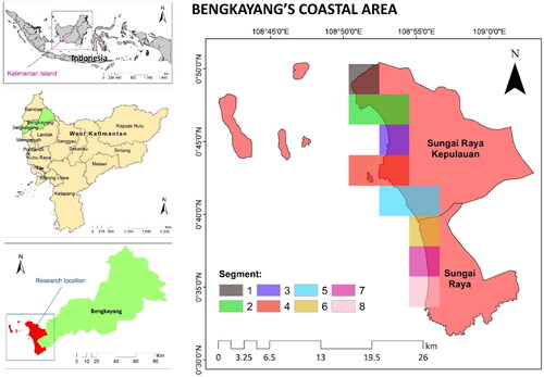
Table 1. Dataset and research variables.

Variable	Source
Shoreline (Y)	Historical maps and Landsat imageries – United States Geological Surveys (USGS)
Total suspended solids (X1)	Landsat imageries – United States Geological Surveys (USGS)
Underwater slope (X2)	National Bathymetry (BatNas) – Indonesian Geospatial Agency (BIG)
Depth (X3)	National Bathymetry (BatNas) – Indonesian Geospatial Agency (BIG)
Distance from the estuaries (X4)	Very high-resolution satellite Imageries interpretation and field survey – Maxar Technologies Inc.
Wind speed (X5)	European Center for Medium-Range Weather Forecasts
Distance from the coastal constructions (X6)	Very high-resolution satellite Imageries interpretation and field survey – Maxar Technologies Inc.

The collection of information in accordance with the needs of the research requires that the data complete the preprocessing stages involving imagery correction as well as reprojection. The historical maps must be corrected by their coordinates. To minimize geometric errors, the historical maps need to rectify based on the geographical objects which have a steady state in a long-term period, such as three-way junctions or intersection roads, crossroads, peak of hills or mountains, etc. Some data also need to be processed further such as the shoreline extraction where the normalized difference water index (NDWI) and modified difference water index (MNDWI) were applied as shown in Equations 1(1) $$\text{NDWI}=\frac{\text{NIR}\mathrm{ }-\mathrm{ }\text{SWIR}}{\text{NIR}\mathrm{ }+\mathrm{ }\text{SWIR}}$$(1) and 2(2) $$\text{MNDWI}=\frac{\text{GB}\mathrm{ }-\mathrm{ }\text{SWIR}}{\text{GB}\mathrm{ }+\mathrm{ }\text{SWIR}}$$(2) (Mancino et al. 2020). Our research not applied tidal correction because, there is an insignificant effect of the tide on the shoreline changes for coastal areas facing Karimata Strait and Java Sea (Wicaksono et al. 2018; Pampanglola and Handoko 2019). This study proposed thresholds of 0.005 for Landsat-3 MSS 1981, 0.003 for Landsat-5 TM 1991, 0.080 for Landsat-7 ETM+ 2001, 0.065 for Landsat-5 TM 2011, and 0.070 for Landsat-8 OLI 2021. Moreover, the NDWI was able to distinguish water and land features, thereby, making it easy to conduct the delineation and classification. It was also possible to obtain the TSS from Landsat TM, ETM, and OLI satellite imagery as indicated by Parwati and Purwanto (2017) algorithm while Landsat MSS satellite imagery used the algorithm from Topliss et al. (1990). The two have high accuracy for surface TSS estimation as presented in Equations 3(3) $${\text{TSS}}_{\text{(mg/l)}}\text{= 0}\text{.6211×(7}\text{.9038×Exp (23}{\text{.942×RB))}}^{\text{0}\text{.9645}}$$(3) and 4(4) $${\text{TSS}}_{\text{(mg/l)}}\text{= 1}\text{.4×}{\left(\text{B5 / B6}\right)}^{\text{2}}\text{– 6}\text{.2×}\left(\text{B5 / B6}\right)\text{ + 10}\text{.8}$$(4) . Meanwhile, the underwater slope data were obtained from the difference in height and distance from two different points (percentage) such that a higher value indicates a steeper surface and vice versa (Robaina and Trentin 2020). (1) $$\text{NDWI}=\frac{\text{NIR}\mathrm{ }-\mathrm{ }\text{SWIR}}{\text{NIR}\mathrm{ }+\mathrm{ }\text{SWIR}}$$(1) (2) $$\text{MNDWI}=\frac{\text{GB}\mathrm{ }-\mathrm{ }\text{SWIR}}{\text{GB}\mathrm{ }+\mathrm{ }\text{SWIR}}$$(2) (3) $${\text{TSS}}_{\text{(mg/l)}}\text{= 0}\text{.6211×(7}\text{.9038×Exp (23}{\text{.942×RB))}}^{\text{0}\text{.9645}}$$(3) (4) $${\text{TSS}}_{\text{(mg/l)}}\text{= 1}\text{.4×}{\left(\text{B5 / B6}\right)}^{\text{2}}\text{– 6}\text{.2×}\left(\text{B5 / B6}\right)\text{ + 10}\text{.8}$$(4)

Where, NDWI is the normalized difference water index, NIR is the near-infrared band, SWIR is the short-wave infrared band, MNDWI is the modified difference water index, GB is the green band, TSS is the surface total suspended solids, RB is the red band (for Landsat TM, ETM+, and OLI), Exp is an exponential function, while B5 and B6 are band numbers from Landsat MSS imagery.

2.2. Data analysis

Shoreline changes are divided into three types which include accretion, abrasion, and static based on their direction from the land (Achmad et al. 2020). The relationship between the independent and dependent variables in the shoreline process was analyzed using multiple linear regression (Equation 5(5) $$\mathrm{Y}=\mathrm{a}+{\mathrm{b}}_1{\mathrm{X}}_1+{\text{ b}}_2{\mathrm{X}}_2\mathrm{\dots }.+{\mathrm{b}}_{\mathrm{n}}{\mathrm{X}}_{\mathrm{n}}$$(5) ). The significance of the interaction was determined simultaneously with reference to F-statistic, r-value, and p-value while the partial model was based on the t-value. Moreover, the whole of Bengkayang’s coastal area was examined but the interaction in each segment was the focus in order to determine the dominant influencing factors. It is also important to note that the analysis does not only focus on the past and present but also applied some models to determine the future development of shoreline changes between 2031 and 2041. This indicates the geospatial analysis was used to evaluate the past and current situations and the findings were further applied to modeling future phenomena (Dede et al. 2021). The shoreline dynamics analysis was conducted based on 1) end point rate (EPR), 2) linear regression rate (LRR), 3) LR2 (r-square of linear regression), 4) shoreline change envelope (SCE), 5) net shoreline movement (NSM), and 6) standard error of linear regression (LSE) from the digital shoreline analysis system (DSAS), EPR and LRR formula are shown by Equations 6(6) $$\mathrm{Y}=\frac{{\mathrm{L}}_1-{\mathrm{L}}_2}{{\mathrm{t}}_1-{\mathrm{t}}_2}$$(6) and 7 (Nassar et al. 2019; Chrisben Sam and Gurugnanam 2022). Also, shoreline changes for the regression model referred to buffering analysis (Heo et al. 2009; Aladwani 2022). Quantitative analysis always requires normally distributed data, therefore, the distribution of the data used was determined using Kolmogorov-Smirnov (KS) test (Widiawaty et al. 2022) which showed that the p-value was 0.73 at a 95% confidence level and this signifies the data are normally distributed since the p-value is more than 0.05. These results serve as the foundation for further analysis to determine the changes in the shoreline of Bengkayang coastal areas. (5) $$\mathrm{Y}=\mathrm{a}+{\mathrm{b}}_1{\mathrm{X}}_1+{\text{ b}}_2{\mathrm{X}}_2\mathrm{\dots }.+{\mathrm{b}}_{\mathrm{n}}{\mathrm{X}}_{\mathrm{n}}$$(5) where Y is the dependent variable, a is the regression constant, b is the slope of line (regression coefficient). (6) $$\mathrm{Y}=\frac{{\mathrm{L}}_1-{\mathrm{L}}_2}{{\mathrm{t}}_1-{\mathrm{t}}_2}$$(6) (7) $$\mathrm{Y}=\mathrm{b}+\text{mx}$$(7) where L₁ and L₂ is the distance separating between shoreline and baseline, t₁ and t₂ is the dates (period) of the shoreline positions, L represents the distance from the base line, x shoreline dates interval (years), and m is the slope of fitted line, b is y-intercept of regression. LRR is determined by a least squares regression to all shoreline transects, hence the upcoming shoreline positions are predicted based on this method.

3. Results

3.1. Shoreline changes

Shoreline changes in Bengkayang are very dynamic between accretion and abrasion using 1945 as the baseline as indicated in Figure 2. Accretion occurred in 1981, 1991, and 2021, with abrasion detected in 2001 and 2011. The shoreline between 1981–1991 was observed to be quite stable because there were almost no significant changes from the baseline as shown in Table 2 because the distance in this period relatively closest. Meanwhile, abrasion was detected in 2001 and was also able to blow the lands from the accretion in the previous period at an average of −18.64 meters and a median of −35.15 meters. The situation started when the abrasion decreased in 2011 with continuous land loss by the seawater as indicated by the baseline. Lands from accretion were used as mangrove and salting or embankment areas (Ilman et al. 2016). The situation started changing in 2021 with the accretion observed to have caused an increment in the land by 37.05 meters. This addition enhanced the awareness of the government, community, and other stakeholders concerning the vegetative and geotechnical restoration of coastal ecosystems along West Kalimantan (Kusmana 2014; Richards and Friess 2016). However, the pattern of the shoreline changes has striking differences in each segment as indicated in Figure 3 with only 4 segments discovered to have accretion trends while the others showed abrasion trends.

Figure 2. Actual shoreline changes in Bengkayang Regency.

Figure 3. Shoreline changes in each segment measured as average and median values based on the baseline. The accretion is represented by positive values while abrasion is through negative values. Segments 1–4 showed accretion, but segments 6–7 had abrasions. Stable shorelines with a tendency to abrasion appeared in segments 1 and 5. Segment 8 occurred reversal from accretion to abrasion.

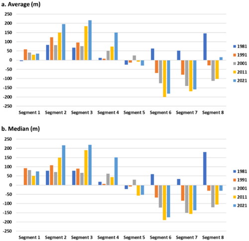
Table 2. Summary of shoreline changes from the baseline based on the buffering analysis.

Year	Abrasion (m)			Accretion (m)			Gain and Loss (m)		Change Rate (m per year)
	Mean	Median	SD	Mean	Median	SD	Mean	Median	Mean	Median
1981	68.74	60.00	48.29	100.69	90.00	59.47	31.95	30.00	0.89	0.83
1991	79.13	67.08	44.58	100.27	90.00	59.54	21.14	22.92	0.46	0.50
2001	114.65	120.00	61.41	96.01	84.85	60.84	−18.64	−35.15	−0.33	−0.63
2011	146.78	150.00	74.41	136.45	134.16	68.67	−10.33	−15.84	−0.16	−0.24
2021	137.26	134.16	68.58	174.31	182.48	90.61	37.05	48.32	0.49	0.64

Segments 1–4 are further north and receive protection from small islands than segments 5–6 which are facing the ocean directly. Segment 1 has the least accretion despite experiencing an abrasion in 1981. This is certainly different from segments 2 and 3 with the farthest land addition reaching more than 200 meters from the baseline in 2021. Moreover, the fastest accretion occurred in segment 4 with a 50–100 meters increment in the last 10 years (2011–2021) while segments 5–8 showed a fairly common occurrence of abrasion up to the present moment except for segment 5 which obtained land from accretion in 1981. It was discovered that segment 8 is the most dynamic area as indicated by repeated accretion between 1981 and 2021. There is also actually quite a bit of abrasion in segment 5, these areas are both headlands with the potential to become suspension deposits in the coastal areas. This is in line with the previous argument that an area does not get hit by waves, winds, and high ocean currents commonly known as deposit zones (Vargas et al. 2016; Goodwin et al. 2020).

3.2. Factors affecting shoreline changes

Shoreline changes in Bengkayang are commonly influenced by three factors which include coastal constructions, underwater elevation (depth), and river estuary. These factors together have 22 percent (r-value 0.47) determination with a p-value < 0.01 at the 95% confidence level as presented in Table 3. It was also discovered that coastal constructions have a positive influence on shoreline changes while depth and river estuary on the contrary have a negative influence as indicated by the t-values in Table 4. This implies the coastal areas close to several coastal constructions have the ability to hold and deposit sediment and ocean currents, thereby, leading to the occurrence of accretion (Widiawaty et al. 2021). The negative effects of underwater elevation (depth) are more dominant in shallow areas of Bengkayang and this further significantly influences sediment supplies from several river estuaries. The findings from the locations that are relatively far from the estuaries showed that the areas have relatively little changes in the coastal landscape as indicated in Figure 4. The statistical analyses conducted also showed that the constant for the regression model developed is significant (p-value < 0.01, 95% confidence level).

Figure 4. Several factors proposed to be affecting the shoreline changes.

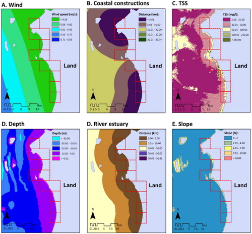
Table 3. Simultaneous interaction of factors affecting the shoreline changes in Bengkayang.

r-value	r-square	p-value	F-Stats	DoF
0.47	0.22	<0.01	12.12	257(6)

Table 4. Regression constant for the simultaneous interaction.

Variable	β	SE	t-value	p-value
Constant	1.75	0.38	4.58	<0.01
Wind	−2.22	1.15	−1.93	0.05
Coastal construction	0.08	0.01	7.40	<0.01
TSS	−0.08	0.04	−1.97	0.05
Elevation (depth)	−0.05	0.02	−2.28	<0.05
River estuary	−0.09	0.02	−4.01	<0.01
Slope	0.06	0.04	1.75	0.08

The factors affecting the shoreline of Bengkayang were observed to have different interactions when viewed by each segment. A detailed understanding of this interaction per segment is very important in coastal management to develop appropriate policies to prevent damage to the ecosystems and communities (Boak and Turner 2005; Ankrah et al. 2022). Moreover, Table 5 showed there are six segments with significant interactions between bio-geophysical and anthropogenic factors as indicated by p-value < 0.01 (95 confidence level) except for segments 1 and 5. The regression model, r-value, was also able to show a significant relationship between independent and dependent variables up to 0.86 for segment 3 while segments 7 and 8 had very high and significant values of 0.83 and 0.84 respectively. The other three segments also have high values which are higher than 0.70 but this does not guarantee significant interactions between the variables in segment 5 because the F-statistic does not meet the threshold value in the F-table (Nurbayani and Dede 2022).

Table 5. Interaction of factors affecting the shoreline changes in each segment.

Segment	r-value	r-square	p-value	F	DoF
1	0.62	0.38	0.06	2.4	23(6)
2	0.76	0.58	<0.01	8.84	38(6)
3	0.86	0.74	<0.01	15.77	33(6)
4	0.74	0.55	<0.01	6.59	32(6)
5	0.78	0.61	0.64	0.77	3(6)
6	0.75	0.56	<0.01	6.5	31(6)
7	0.83	0.69	<0.01	9.56	26(6)
8	0.84	0.71	<0.01	9.1	22(6)

The partial interaction between variables which is previously stated to be significant was determined for each segment, but segment 3 have higher interactions with four factors including wind, coastal constructions, TSS, and river estuaries discovered to be influencing the shoreline changes as presented in Table 6. Another segment with accretion showed certain differences and this is probably associated with the fact that segment 3 has three significant factors which are wind, elevation (depth), and river estuary while segment 4 has only TSS. Moreover, it was also discovered that only the river estuaries have a positive regression coefficient out of all the factors and this confirms that rivers with high sediment loads and turbidity can shallow up to the moment the water rises and land emerges (Kamarudin et al. 2020). Meanwhile, several conditions such as low wind speed, shallow water, and coastal engineering have the ability to move the shoreline towards the ocean. This is indicated by the locations with abrasion trends where only segments 7 and 8 have partial interactions. The underwater slope showed a significant role in segment 7 but wind and river estuaries played a dominant role in shoreline changes in segment 8 as presented in Table 7. The slope became the main differentiator because it was the only non-significant factor in the accretion process. Furthermore, the underwater slope makes it easier for seawater to erode the land, especially when the soil has not been strongly consolidated (Van Rijn 2011; Mickovski et al. 2015). There is a need for more investigation into wind and TSS because the shoreline changes in segment 8 showed a reversal pattern from abrasion to accretion.

Table 6. Regression constant in segments 1–4.

Variable	Segment 1			Segment 2			Segment 3			Segment 4
	β	SE	t-value	Β	SE	t-value	β	SE	t-value	β	SE	t-value
Constant	5.70	4.09	1.40	−6.96	1.69	−4.13**	13.55	2.49	5.43**	−13.37	9.27	−1.44
Wind	9.43	10.82	0.87	−29.37	5.28	−5.56**	27.43	6.75	4.07**	−31.88	12.23	−2.61*
Coastal construction	−0.08	0.09	−0.84	−0.01	0.04	−0.20	−0.70	0.15	−4.74**	1.80	1.33	1.35
TSS	0.24	0.13	1.84	−0.17	0.11	−1.53	−0.35	0.09	−3.83**	−0.43	0.15	−2.82**
Elevation (depth)	−0.25	0.15	−1.67	−0.12	0.04	−2.72*	0.08	0.05	1.86	−0.09	0.07	−1.37
River estuary	−0.30	0.30	−1.00	0.32	0.09	3.64**	0.11	0.03	3.78**	0.10	0.22	0.46
Slope	0.24	0.24	1.01	0.16	0.08	2.00	0.00	0.04	−0.07	−0.13	0.14	−0.90

* Significance with p-value below 0.05 and confidence level 95%.

** Significance with p-value below 0.01 and confidence level 95%.

Table 7. Regression constant in segments 5–8.

Variable	Segment 5			Segment 6			Segment 7			Segment 8
	Β	SE	t-value	Β	SE	t-value	β	SE	t-value	β	SE	t-value
Constant	22.03	17.14	1.29	−14.43	8.32	−1.73	4.90	4.49	1.09	−14.90	3.04	−4.90**
Wind	45.45	37.29	1.22	−51.38	26.42	−1.95	7.73	14.61	0.53	−59.92	10.16	−5.90**
Coastal construction	−1.83	1.57	−1.17	0.20	0.14	1.41	−0.02	0.07	−0.24	0.22	0.11	2.06
TSS	0.19	0.13	1.42	−0.08	0.06	−1.47	0.03	0.18	0.14	0.04	0.12	0.29
Elevation (depth)	0.12	0.24	0.50	0.02	0.08	0.20	0.07	0.04	1.89	−0.10	0.05	−2.01
River estuary	0.13	0.26	0.50	0.05	0.11	0.47	−0.05	0.08	−0.61	−0.40	0.10	−3.86**
Slope	0.04	0.10	0.38	0.07	0.05	1.42	−0.40	0.10	−3.86**	−0.13	0.15	−0.86

* Significance with p-value below 0.05 and confidence level 95%.

** Significance with p-value below 0.01 and confidence level 95%.

3.3. Bengkayang’s shorelines in the future

The shoreline is projected to have an abrasion trend of 25–27 meters average and 18–29 meters median inland compared to the 1945 baseline. This is expected to reduce land mass by 211.52 meters and 244.04 meters in 2031 and 2041 respectively and these are greater than the potential accretions which are projected to be 186.46 meters and 217.60 meters for the same period. This means the coastal landscape of Bengkayang has relatively no significant change for 96 years because the annual rate is less than one meter. However, the future shoreline changes are very dynamic and differ in each segment in terms of spatial distribution as presented in Figure 5 and Table 8. The modelling results show that segment 1 is the most stable because the value of shoreline change due to accretion is less than 50 meters during the study period and also has a median value which is not more than 100 meters. Whereas, segments 2 and 4 also have accretion tendencies but they are very different from segment 1 due to their ability to add mass up to 194–293 meters towards the sea. This information can be utilized by the government and private development proponents in developing the coastal areas despite the threat of sea-level rise and land subsidence (Devoy 2008; Griggs and Reguero 2021). Moreover, the efforts to handle accretion, especially those with a very small value, are relatively easier in terms of technicality, cost, and social challenges compared to dealing with abrasion.

Figure 5. Potential shoreline changes in Bengkayang Regency.

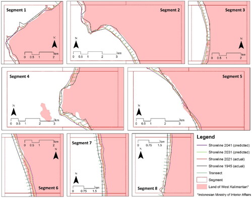
Table 8. Future shoreline changes in each segment of the Bengkayang Regency.

Segment	Year	Abrasion (m)			Accretion (m)			Gain and loss (m)		Change Rate (m per year)
		Mean	Median	SD	Mean	Median	SD	Mean	Median	Mean	Median
1	2031	127.24	84.85	92.58	171.95	161.55	80.90	44.71	76.70	0.52	0.89
	2041	136.33	94.87	96.00	171.17	152.97	80.44	34.84	58.10	0.36	0.61
2	2031	0.00	0.00	0.00	213.71	231.39	89.85	213.71	231.39	2.49	2.69
	2041	0.00	0.00	0.00	237.64	268.33	101.93	237.64	268.33	2.48	2.80
3	2031	0.00	0.00	0.00	252.41	270.00	41.13	252.41	270.00	2.94	3.14
	2041	0.00	0.00	0.00	292.96	300.75	41.75	292.96	300.75	3.05	3.13
4	2031	0.00	0.00	0.00	194.43	192.09	106.82	194.43	192.09	2.26	2.23
	2041	0.00	0.00	0.00	226.44	234.31	126.81	226.44	234.31	2.36	2.44
5	2031	143.51	155.78	70.41	92.13	67.08	69.08	−51.38	−88.70	−0.60	−1.03
	2041	172.37	189.74	99.44	119.74	84.85	98.40	−52.63	−104.89	−0.55	−1.09
6	2031	270.42	247.39	49.90	0.00	0.00	0.00	−270.42	−247.39	−3.14	−2.88
	2041	323.65	307.40	62.43	0.00	0.00	0.00	−323.65	−307.40	−3.37	−3.20
7	2031	238.16	240.00	55.28	0.00	0.00	0.00	−238.16	−240.00	−2.77	−2.79
	2041	276.60	256.32	66.10	0.00	0.00	0.00	−276.60	−256.32	−2.88	−2.67
8	2031	178.60	180.00	89.68	61.98	30.00	59.43	−116.62	−150.00	−1.36	−1.74
	2041	184.73	210.00	116.17	129.56	135.00	65.86	−55.17	−75.00	−0.57	−0.78

Segments 6 and 7 have the potential for strong abrasion with the possibility of retreating for more than 200 meters by 2031. Both segments are also projected to have a land mass reduction of more than 250 meters by 2041 which is the highest since 1941. This is obviously a real threat that needs serious attention from relevant parties to ensure the coastal landscape does not suffer big losses and be eroded up to 3 meters per year. In contrast, segments 5 and 8 have the potential to experienced abrasion with lower intensity in the next two periods with segment 5 having an average of 50 meters which means the loss rate is still below 2 meters per year. A different trend is projected to occur in segment 8 because the abrasion in the 2031 period can reduce the land by more than 50 percent and bring significant impact on the coastal community, especially to the fishing communities in reducing the accessibility to the catching areas. This implies there is probably going to be an increasing shift away from the resources normally used for livelihoods and the possibility of siltation impacting the littoral zone (Widiawaty et al. 2020).

The shoreline changes in Bengkayang are quite diverse in each segment even though it was generally observed that there was an abrasion rate. Moreover, the actual coastal landscape, from 1945–2021, showed stability because the abrasion during the period has started to be replaced by the latest accretion. It was further indicated that the smallest EPR with both positive and negative notations is associated with segments 1 and 5 in Figure 3 and this is similar to the SCE value where segment 1 changed by only 85.95 meters during the actual observation period, thereby, having the tendency to increase land mass. Meanwhile, the most dynamic segments with different contexts are segment 4 with accretion and segment 6 with abrasion as indicated by SCE value 192.13 meters as shown in Table 9. This signifies the two segments are not suitable for development in Bengkayang in terms of marine and fisheries resources despite efforts to implement coastal engineering in the regency. It is also important to remember that the infrastructure to cope with shoreline dynamics requires high-cost for its rapid construction ​​including coastal engineering and protection from extreme weather (Hakim 2017; Aerts 2018; Susilawati and Mefianti 2018). Furthermore, the lowest value for NSM was recorded in segments 1 and 5 with less than 10 meters. These three parameters confirmed that segment 1 requires efforts to overcome accretion while segment 5 requires handling the abrasion as shown in Figure 6. The other segments are not ignored in the process even though they are not the focus of developmental activities on the national scale. It is important to note that abrasion and accretion can be seen as an equilibrium process requirements comprehensive-integrative management (Prasetya 2007; Yates et al. 2009).

Figure 6. Detail of shoreline dynamics in each segment.

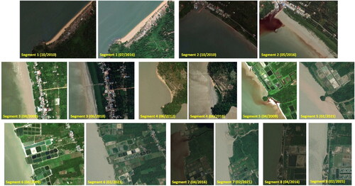
Table 9. Statistical parameters of shoreline changes.

Segment	EPR	LRR	LR2	SCE	NSM	LSE
1	−0.06	−0.35	0.4	85.95	−4.48	32.66
2	1.45	2.95	0.47	180.58	110.46	58.7
3	1.78	3.86	0.72	144.4	135.39	40.89
4	2.86	5.37	0.66	309.69	217.26	61.08
5	0.11	1.09	0.6	139.88	8.34	33.35
6	−3.22	−6.4	0.83	256.12	−244.73	43.77
7	−3.14	−5.53	0.72	252.46	−238.54	63.58
8	−2.91	−4.97	0.49	261.31	−220.78	89.24

4. Discussion

Shoreline dynamics requires understanding the changing trend as indicated by the LRR, LR2, and LSE which are derivatives of the linear statistical model (Himmelstoss 2009). The findings showed that the Bengkayang’s shoreline has LRR −0.02 and this means the slope of the regression line tends toward abrasion. This is associated with the fact that the segments with negative values ​​are greater than those with positive values. In line with the LR2 value, the abrasion in segment 6 has a very high trend of determination with 0.83 while segment 8 is most clearly characterized by the reversal from abrasion to accretion or vice versa which is known as cyclical trends. Therefore, the LSE for segment 8 is the largest compared to the others, especially in areas with coastal landscape stability trends. It is important to note that the existence of a large LSE value in one segment, especially with a significant difference from the average LSE for the entire study area, is a sign to have more observations with short periods ranging from 1–5 years in order to improve the shoreline changes model. However, the current model can be used as a reference due to its good accuracy as indicated by the standard error of the estimate measures and its ability to meet the criteria for validity and reliability in the range of 30–80 meters which is considered effective for spatial resolution of Landsat series imageries from MSS to OLI sensors (Ozesmi and Bauer 2002; Salehi et al. 2021).

It was discovered that segments 1 and 5 need to focus on the angle direction of the shoreline changes in areas with a stable coastal landscape. The data showed that segment 1 has an abrasion direction from the north (1°) and has the potential to shift to the northeast (50.43°) in the future. The increase in land mass between 1945–2021 was found in the southeast direction (155.12°) but projected to change to the northwest (338.28°) in the next decade. Meanwhile, the actual abrasion in segment 5 originates from the southeast (143.62°) and the sea is projected to erode the land from the northwest (321.26°) in the future. These segments were not significantly affected by the shoreline determinant factors formulated in this research. The coastal features in segment 1 such as some headlands were able to intercept and deflect the currents in order to reduce the abrasion-accretion phenomenon (Ruggiero et al. 2013; Van den Broeck 2017). However, segment 5 is relatively more protected from the determinants concentrated in the other five segments, in both the north and south directions, and this encourages fewer shoreline changes. It is also important to state that accretion is concentrated in a bay-shaped coastal area with two headlands and several sea stacks or small islands in segments 2 and 4. The appearance of spits and sand bars is a common phenomenon due to the deposition of fluvio-marine sediments (Mujabar and Chandrasekar 2012; Rutten et al. 2018).

Due to the dynamic nature of the coastal zone, the accretion and abrasion in Bengkayang Regency need proper handling in accordance with the best practices in coastal area management. The approach to protect the coast from abrasion needs to prioritize conservation and rehabilitation strategies and also consider local environmental characteristics such as sandy, muddy, or rocky areas along with the history of the shoreline (Lee et al. 2014; Mohamad et al. 2014; Noor and Maulud 2022). The adaptation and prevention costs are lower than the environmental and socio-economic damages due to abrasion or accretion. Moreover, there is a need for appropriate engineering efforts in segments with the known occurrence of shoreline dynamics to determine the causative factors. The strategies intended to conserve and rehabilitate the shorelines also need to consider the socio-economic aspects in order to ensure the surrounding community enjoys these results. The latest methods considered more environmentally friendly such as the combination of civil engineering with vegetation plantation need to be applied to fill the lost areas due abrasion. This approach, however, requires further and detailed observations, especially concerning the characteristics of the sediment (budgets), land and water topography, waves, ocean currents, ecosystem behavior, livelihoods, and the origin of materials. This is important because the efforts to protect coastal ecosystems through only engineering measures such as sea dikes have been unable to resolve the shoreline dynamics challenges in Jakarta, Pekalongan, and Semarang (Marfai 2014; Harini et al. 2017).

5. Conclusion

The shoreline in Bengkayang increased by 37.05 meters to the sea between 1941 and 2021. Accretion was observed to have occurred in segments 1–4 with the highest in 2–4, thereby, forming emerged lands up to over 100 meters while abrasion was in segments 5–8 and eroded the land mass in 6–8 by 100–200 meters. The most stable shoreline was found to be segments 1 and 5 even though they both have relatively small accretion and abrasion. Whereas, shoreline reversal occurred in segment 8 with an accretion-abrasion-accretion pattern at a different rate every 10 years. It was also discovered that the shoreline dynamics in the regency are significantly influenced by three factors which are the coastal constructions, underwater elevation (depth), and river estuaries. However, a combination of six different factors was observed to be driving the dynamics in each segment. The multiple linear regression model showed an influence of 22 percent (r-value 0.47) from bio-geophysical and anthropogenic factors. The model has several determinations in each segment with an interval of 38–71 percent which includes significant accretion in segments 2–4 and abrasion in 6–8. The projection showed that Bengkayang’s shoreline is also dynamic in the future, but the land mass is expected to be reduced by 211.52 meters in 2031 and 244.04 meters in 2041 due to accretion. These dynamics are a challenge for coastal development and management in the regency and an adequate understanding of accretion and abrasion is significantly required in formulating policies to achieve prosperity for the surrounding community and environment. The threat needs to be addressed with the latest approach that combines engineering, ecosystem, social, and economic aspects in order to ensure the achievement of sustainability goals related to the environmental, political, social, and economic aspects without any unequal interests.

Authors’ contributions

All authors contributed equally in this work.

Acknowledgements

This study was funded by Indonesian Government Research in 2021. It was managed by the Center for Nuclear Energy System Assessment National Nuclear Energy Agency of Indonesia (BATAN) and BRIN. It was also partially supported by RISTEK/BRIN-LPDP project (14/E1/III/PRN/2021) and Universiti Kebangsaan Malaysia research grant (GP-2021-K006900). The authors would like to thank the anonymous reviewers for their comments.

Data availability

The datasets are available from the corresponding author on reasonable request.

Disclosure statement

The authors declare there is no conflict of interest.

References

- Achmad E, Nursanti N, Fazriyas F, Jayanti, DP, Marwoto. 2020. Studi kerapatan mangrove dan perubahan garis pantai tahun 1989-2018 di Pesisir Provinsi Jambi. JPSL. 10(2):138–152.
- Aerts JC. 2018. A review of cost estimates for flood adaptation. Water. 10(11):1646.
- Akbar AA, Sartohadi J, Djohan TS, Ritohardoyo S. 2017. The role of breakwaters on the rehabilitation of coastal and mangrove forests in West Kalimantan, Indonesia. Ocean Coast Manage. 138:50–59.
- Aladwani NS. 2022. Shoreline change rate dynamics analysis and prediction of future positions using satellite imagery for the southern coast of Kuwait: a case study. Oceanologia. 64(3):417–432.
- Amukti R, Adji AS, Ruslan S. 2020. Analysis of shoreline shift using satellite imagery near Makassar City. J Geoscience Eng Environ Technol. 5(3):133–138.
- Ankrah J, Monteiro A, Madureira H. 2022. Bibliometric analysis of data sources and tools for shoreline change analysis and detection. Sustainability. 14(9):4895.
- Azhar MM, Maulud KNA, Selamat SN, Khan MF, Jaafar O, Jaafar WSWM, Abdullah SMS, Toriman ME, Kamarudin MKA, Gasim MB, et al. 2018. Impact of shoreline changes to the coastal development. IJET. 7(3.14):191–195.
- Boak EH, Turner IL. 2005. Shoreline definition and detection: a review. J Coast Res. 214(4):688–703.
- Dede M, Asdak C, Setiawan I. 2021. Spatial dynamics model of land use and land cover changes: a comparison of CA, ANN, and ANN-CA. Regist j Ilm Teknol Sist Inf. 8(1):38–49.
- Devoy RJ. 2008. Coastal vulnerability and the implications of sea-level rise for Ireland. J Coast Res. 242(2):325–341.
- Directorate of Spatial Planning and Land Affairs [DSPLA] 2015. Spatial profile of West Kalimantan. Jakarta, Indonesia: Indonesian Ministry of National Development Planning.
- ervita K, Marfai MA. 2017. Shoreline change analysis in Demak, Indonesia. JEP. 08(08):940–955.
- Gonçalves G, Santos S, Duarte D, Gomes J. 2019. Monitoring Local Shoreline Changes by Integrating UASs, Airborne LiDAR, Historical Images and Orthophotos. Proceedings of the 5th International Conference on Geographical Information Systems Theory, Applications and Management (GISTAM). Scitepress.
- Goodwin ID, Ribó M, Mortlock T. 2020. Coastal sediment compartments, wave climate and centennial-scale sediment budget. Sandy Beach Morphodynamics. Amsterdam: elsevier.
- Gopinath G, Seralathan P. 2005. Rapid erosion of the coast of Sagar island. Environ Geol. 48(8):1058–1067.
- Griggs G, Reguero BG. 2021. Coastal adaptation to climate change and sea-level rise. Water. 13(16):2151.
- Chrisben Sam S, Gurugnanam B. 2022. Coastal transgression and regression from 1980 to 2020 and shoreline forecasting for 2030 and 2040, using DSAS along the southern coastal tip of Peninsular India. Geodesy and Geodynamics. 13:585–594.
- Hakim LL. 2017. [Cost and benefit analysis for coastal management: A case study of improving aquaculture and mangrove restoration management in Tambakbulusan Village Demak Indonesia]. [Master Thesis]. Wageningen University and Research Centre. https://library.wur.nl/WebQuery/theses/2217619.
- Harini R, Susilo B, Sarastika T, Supriyati S, Satriagasa MC, Ariani RD. 2017. The survival strategy of households affected by tidal floods: the cases of two villages in the Pekalongan coastal area. For Geo. 31(1):163–175.
- Harley MD, Kinsela MA, Sánchez-García E, Vos K. 2019. Shoreline change mapping using crowd-sourced smartphone images. Coast Eng. 150:175–189.
- Hassan MI, Rahmat NH. 2016. The effect of coastline changes to local community’s social-economic. Int Arch Photogramm Remote Sens Spatial Inf Sci. XLII-4/W1:25–36.
- Heo J, Kim JH, Kim JW. 2009. A new methodology for measuring coastline recession using buffering and non‐linear least squares estimation. Int J Geograph Inf Sci. 23(9):1165–1177.
- Himmelstoss EA. 2009. DSAS 4.0 installation instructions and user guide. Digital Shoreline Analysis System (DSAS) version 4.0 — An ArcGIS Extension for Calculating Shoreline Change: u.S. Geological Survey Open-File Report 2008-1278. Washington: united States Geological Survey.
- Ilman M, Dargusch P, Dart, P, Onrizal. 2016. A historical analysis of the drivers of loss and degradation of Indonesia’s mangroves. Land Use Policy. 54:448–459.,
- Ismail SZ, Zulkifley MA, Hussain A, Mustafa MM, Muad AM. 2017. Automated shoreline detection using natural colour composite on SPOT 5 satellite imagery. Adv Sci Lett. 23(5):4601–4604.
- Jana A, Maiti S, Biswas A. 2016. Analysis of short-term shoreline oscillations along Midnapur-Balasore Coast, Bay of Bengal, India: a study based on geospatial technology. Model Earth Syst Environ. 2(2):1–10.
- Jana A, Maiti S, Biswas A. 2016. Seasonal change monitoring and mapping of coastal vegetation types along Midnapur-Balasore Coast, Bay of Bengal using multi-temporal Landsat data. Model Earth Syst Environ. 2(1):1–12.
- Jana A, Maiti S, Biswas A. 2017. Appraisal of long-term shoreline oscillations from a part of coastal zones of Sundarban delta, Eastern India: a study based on geospatial technology. Spat Inf Res. 25(5):713–723.
- Kamarudin MKA, Abd Wahab N, Abu Samah MA, Baharim NB, Mostapa R, Umar R, Maulud KNA, Arifin MH, Saad MHM, Bati SNAM. 2020. Potential of field turbidity measurements for computation of total suspended solid in Tasik Kenyir, Terengganu, Malaysia. DWT. 187:11–16.
- Karlonienė D, Pupienis D, Jarmalavičius D, Dubikaltinienė A, Žilinskas G. 2021. The impact of coastal geodynamic processes on the distribution of trace metal content in sandy beach sediments, South-Eastern Baltic Sea coast (Lithuania). Appl Sci. 11(3):1106.
- Kim H, Lee SB, Min KS. 2017. Shoreline change analysis using airborne LiDAR bathymetry for coastal monitoring. J Coast Res. 79:269–273.
- Kumar PD, Gopinath G, Laluraj CM, Seralathan P, Mitra D. 2007. Change detection studies of Sagar Island, India, using Indian remote sensing satellite 1C linear imaging self-scan sensor III data. Journal of Coastal Research. 23(6):1498–1502.
- Kumar PD, Gopinath G, Murali RM, Muraleedharan KR. 2014. Geospatial analysis of long-term morphological changes in Cochin estuary, SW coast of India. J Coast Res. 30(6):1315–1320.
- Kusmana C. 2014. Distribution and current status of mangrove forests in Indonesia. Mangrove ecosystems of Asia. New York: springer.
- Lam KC, Jaafar M, Halime LAR, Asnawi NH, Rose RAC. 2020. Analysis of land use and land cover change of Sidon City, Lebanon. GEOGRAFIA. 16(3):108–130.
- Lee SC, Hashim R, Motamedi S, Song KI. 2014. Utilization of geotextile tube for sandy and muddy coastal management: a review. Sci World J. 2014:494020.
- Lord M, Chang S. 2018. West Kalimantan integrated border area development. MPRA Paper No. 86537. https://mpra.ub.uni-muenchen.de/86537/.
- Mancino G, Ferrara A, Padula A, Nolè A. 2020. Cross-comparison between Landsat 8 (OLI) and Landsat 7 (ETM+) derived vegetation indices in a Mediterranean environment. Remote Sens. 12(2):291.
- Marfai MA. 2014. Impact of sea level rise to coastal ecology: a case study on the northern part of Java Island, Indonesia. Quaestiones Geographicae. 33(1):107–114.
- Maulud KNA, Rafar RM. 2015. August Determination the impact of sea level rise to shoreline changes using GIS. In International Conference on Space Science and Communication (IconSpace 2015) (pp. 352–357). IEEE.
- Mickovski SB, Santos O, Ingunza PMD, Bressani L. 2015. Coastal slope instability in contrasting geo-environmental conditions. Proceedings of the XVI ECSMGE Geotechnical Engineering for Infrastructure and Development. ICE Publishing.
- Mohamad MF, Lee LH, Samion MKH. 2014. Coastal vulnerability assessment towards sustainable management of Peninsular Malaysia coastline. IJESD. 5(6):533–538.
- Mohd FA, Maulud KNA, Begum RA, Selamat SN, Karim OA. 2018. Impact of shoreline changes to Pahang coastal area by using geospatial technology. JSM. 47(5):991–997.
- Mujabar PS, Chandrasekar N. 2012. Dynamics of coastal landform features along the southern Tamil Nadu of India by using remote sensing and Geographic Information System. Geocarto Int. 27(4):347–370.
- Mutaqin BW. 2017. Shoreline changes analysis in Kuwaru coastal area, Yogyakarta, Indonesia: an application of the digital shoreline analysis system (DSAS). Int J SDP. 12(07):1203–1214.
- Nassar K, Mahmod WE, Fath H, Masria A, Nadaoka K, Negm A. 2019. Shoreline change detection using DSAS technique: case of North Sinai coast, Egypt. Mar Georesour Geotechnol. 37(1):81–95.
- Nicholls RJ, Dawson RJ, Day SA. 2015. Broad scale coastal simulation: new techniques to understand and manage shorelines in the third millennium. Dordrecht, Netherlands: Springer.
- Noor NM, Maulud KNA. 2022. Coastal vulnerability: a Brief Review on Integrated Assessment in Southeast Asia. JMSE. 10(5):595.
- Nurbayani S, Dede M. 2022. The effect of COVID-19 on white-collar workers: the DPSIR model and its semantic aspect in Indonesia. Int J Soc Cult Language. 10(2):1–16.
- Ozesmi SL, Bauer ME. 2002. Satellite remote sensing of wetlands. Wetlands Ecol Manage. 10(5):381–402.
- Pampanglola SMNT, Handoko EY. 2019. Estimation of sea-level variability around the Java Sea and Karimata Strait using Cryosat-2 Altimeter. IOP Conf Ser: earth Environ Sci. 389:012021.
- Parwati E, Purwanto AD. 2017. Time series analysis of total suspended solid (TSS) using Landsat data in Berau coastal area, Indonesia. IJReSES. 14(1):61–70.
- Prasetya G. 2007. Protection from coastal erosion (thematic paper: the role of coastal forests and trees in protecting against coastal erosion). Coastal Protection in the Aftermath of the Indian Ocean Tsunami: what Role for Forests and Trees?. Bangkok: FAO Regional Office for Asia and the Pacific. https://www.fao.org/3/ag127e/ag127e00.htm.
- Richards DR, Friess DA. 2016. Rates and drivers of mangrove deforestation in Southeast Asia, 2000–2012. Proc Natl Acad Sci U S A. 113(2):344–349.
- Robaina LEDS, Trentin R. 2020. Automated classification of landforms with GIS support. Mercator-Revista de Geografia da UFC. 19(1):1–16.
- Ruggiero P, Kratzmann MG, Himmelstoss EA, Reid D, Allan J, Kaminsky G. 2013. National assessment of shoreline change: historical shoreline change along the Pacific Northwest coast. US Geological Survey, Washington, USA.
- Rutten J, Ruessink BG, Price TD. 2018. Observations on sandbar behaviour along a man‐made curved coast. Earth Surf Process Landforms. 43(1):134–149.
- Salehi H, Shamsoddini A, Mirlatifi SM, Mirgol B, Nazari M. 2021. Spatial and temporal resolution improvement of actual evapotranspiration maps using Landsat and MODIS data fusion. Front Environ Sci. 9:795287.
- Selamat SN, Maulud KA, Jaafar O, Ahmad H. 2017. Extraction of shoreline changes in Selangor coastal area using GIS and remote sensing techniques. J Phys Conf Ser. 852 012031: 1–9.
- Sunardi S, Nursamsi I, Dede M, Paramitha A, Arief MCW, Ariyani M, Santoso P. 2022. Assessing the Influence of land-use changes on water quality using remote sensing and GIS: a study in Cirata reservoir. Sci Technol Indonesia. 7(1):106–114.
- Susiati H, Dede M, Widiawaty MA, Ismail A, Udiyani PM. 2022a. Site suitability-based spatial-weighted multicriteria analysis for nuclear power plants in Indonesia. Heliyon. 8(3):e09088.
- Susiati H, Widiawaty MA, Dede M, Akbar AA, Udiyani PM. 2022b. Modeling of shoreline changes in West Kalimantan using remote sensing and historical maps. Int J Conserv Sci. 13(3):1043–1056.
- Susilawati S, Mefianti D. 2018. Alternative of coastal erosion countermeasures in Bungin, Luwuk District, Banggai Regency. JTSP. 20(1):41–46.
- Topliss BJ, Almos CL, Hill PR. 1990. Algorithms for remote sensing of high concentration, inorganic suspended sediment. Int J Remote Sens. 11(6):947–966.
- Van den Broeck N. 2017. [Coastal protection with respect to climate change: Practical application on the Belgian coast]. [Master Thesis]. KU Leuven. https://riunet.upv.es/handle/10251/90533.
- Van Rijn LC. 2011. Coastal erosion and control. Ocean Coast Manage. 54(12):867–887.
- Vargas V. H, Uribe E, Castellanos OM, Ríos CA. 2016. Coastal landforms caused by deposition and erosion along the shoreline between Punta Brava and Punta Betín, Santa Marta, Colombian Caribbean. Revista de la Academia Colombiana de Ciencias Exactas Físicas y Naturales. 40(157):664–682.
- Wicaksono A, Wicaksono P, Khakhim N, Mohammad N, Farda MAM. 2018. Tidal correction effects analysis on shoreline mapping in Jepara Regency. JAGI. 2(2):145–151.
- Widiawaty MA. 2019. Mari Mengenal sains informasi geografis. Bandung, Indonesia: Aria Mandiri Group.
- Widiawaty MA, Lam KC, Dede M, Asnawi NH. 2022. Spatial differentiation and determinants of COVID-19 in Indonesia. BMC Public Health. 22(1):1030. 10.1186/s12889-022-13316-4.
- Widiawaty MA, Nandi N, Murtianto H. 2020. Physical and social factors of shoreline change in Gebang, Cirebon Regency 1915–2019. JAGI. 4(1):327–334.
- Widiawaty MA, Nandi N, Murtianto H. 2021. Dampak fisik dan sosial perubahan garis pantai di Kecamatan Gebang, Kabupaten Cirebon. SNG. 4:667–678.
- Wurjanto A, Susiati H, Ajiwibowo H. 2020. Tsunami hazards along coastal area of West Kalimantan Province, Indonesia. GEOMATE. 18(69):151–158.
- Yates ML, Guza RT, O'Reilly WC. 2009. Equilibrium shoreline response: observations and modeling. J Geophys Res. 114(C9):9014–9014.
- Yen NH, Kim, TL. 2020. Coastline changes detection from Sentinel–1 satellite imagery using spatial fuzzy clustering and interactive thresholding method in Phan Thiet, Binh Thuan. Vietnam J Hydrometeorol. 6:1–10.
- Zhang K, Douglas BC, Leatherman SP. 2004. Global warming and coastal erosion. Clim Change. 64(1/2):41–58. CLIM.0000024690.32682.48.