Creep identification by the baseline optimized TS-InSAR technique considering the monthly variation in coherence

Abstract

Time series interferometric synthetic aperture radar (TS-InSAR) technique can be applied to identify the creep body. However, it has strict requirements regarding the quality of the interferograms and the interferometric baseline networks. In regions with intermittent coherence, the use of conventional methods to select interferometric pairs can easily lead to interferometric baseline disconnections, redundancy, or missing key pairs. This results in reduced accuracy and may even misidentify creep characteristics. To solve this problem, the segmented average coherence threshold method (SACTM) is proposed. SACTM is an interferometric baseline optimization method that considers monthly coherence variability. In this paper, the SACTM baseline optimization TS-InSAR technique was used to identify creep bodies in Wudongde Reservoir area located along the Jinsha River in China. Compared with the conventional methods, the SACTM method yields a more robust interferometric baseline network and a smaller standard deviation for deformation rate, which demonstrates the superiority of this method.

Keywords:

• TS-InSAR
• creep
• coherence
• baseline optimization

1. Introduction

A ‘creep body’ is defined as a material block with a slow deformation rate (Wang et al. 2011), such as creeping landslides, creeping material sources of debris flows, or dangerous rock bodies. When affected by rainfall, earthquakes, reservoir storage, human engineering activities and other causal factors, it is easy to develop into creeping geological hazards (Crosta et al. 2013; Kang et al. 2017; Xu et al. 2022). Creep characteristics (creep deformation rate, creep range, etc.) can characterize the movement state of the creep body. Thus, effective identification of creep characteristics can provide important indicators for the prevention and proper risk assessment of creeping geohazards, which is of great importance in the fields of disaster prevention and mitigation.

Compared with traditional ground surveys, optical remote sensing, 3D laser scanning and field engineering investigations (Du and Teng 2007; Nichol and Wong 2005; Sui et al. 2008; Zhang et al. 2007), TS-InSAR technology combines the advantages of wide coverage, low expenditure, high monitoring accuracy and large amount of archived data, and has been widely applied to monitor the spatial and temporal deformation of the Earth’s surface (Cigna and Tapete 2021; Sun and Wang 2018; Xu et al. 2021a; Zhu et al. 2021). However, the complex conjugate multiplication of two SAR images from different periods will yield interferograms of varying quality, and different interferograms can be combined to obtain interferometric baseline networks of varying quality. The TS-InSAR technique has strict requirements regarding the quality of the interferograms (Ansari et al. 2021) and interferometric baseline networks (Braun 2021). In other words, high quality interferograms and robust interferometric baseline networks are prerequisites for effective creep body identification via the TS-InSAR technique; therefore, it is necessary to filter the interferograms and optimize the interferometric baseline network.

At present, the main methods of interferometric baseline optimization are as follows: 1. Manually select interferograms with good coherence based on empirical analysis (Kang et al. 2019). However, the manual selection method requires expert knowledge, is time consuming and labour intensive, and is not suitable for long term deformation monitoring that involves large amounts of data. 2. Interferograms are selected based on short spatio-temporal baseline thresholds (Mohammadimanesh et al. 2019; Zhao et al. 2012). However, short spatio-temporal baseline thresholds cannot eliminate interferograms with short spatio-temporal intervals that have poor coherence, which may introduce decorrelation errors (Lauknes et al. 2011). Furthermore, interferograms that use only short spatio-temporal baselines may introduce systematic errors (Ansari et al. 2021). 3. Interferogram selection may be based on coherence coefficient thresholds (Howard et al. 2022; Kang et al. 2021). The coherence coefficient is determined by the SAR images, spatial baselines, temporal baselines and external environmental factors, which can comprehensively reflect the quality of interferograms (Wang et al. 2022). This method is a more direct and reliable way to optimize the interferometric baselines using the coherence coefficient threshold.

However, the influencing factors of the coherence coefficient, such as soil moisture and vegetation changes, tend to have monthly variations, leading to intermittent coherence issues with interferometric pairs, which makes the threshold of the coherence coefficient difficult to determine. Currently, most studies primarily use uniform custom coherence coefficients (0.3 to 0.6) or average coherence coefficient thresholds (Baran et al. 2005; Santoro et al. 2010; Wang et al. 2022; Zhang et al. 2020). Among these, the selection of interferograms based on the customized coherence coefficient threshold requires advanced knowledge and is subjective. Threshold settings that are too large can easily lead to disconnected or missing interferometric baselines, and disconnected interferometric baselines can lead to reduced accuracy or even unusable deformation inversion results (Braun 2021; Lanari et al. 2004; Lopez-Quiroz et al. 2009). Moreover, missing interferometric baselines will result in too few interferometric pairs, which will not satisfy the TS-InSAR processing requirements (Xu et al. 2021a). Threshold settings that are too small can lead to interferometric baseline redundancy and introduce low-coherence interferometric pairs. Interferometric baseline redundancy will increase the processing difficulty. Additionally, low-coherence interferometric pairs involved in TS-InSAR inversion are prone to introduce decorrelation errors. In summary, processing a large number of interferograms does not always provide a better result (Smittarello et al. 2022). Similarly, using the average coherence coefficient threshold to select interferograms tends to result in missing or disconnected interferometric baselines for low coherence months. Therefore, in the intermittent coherence region, we optimize the interferometric baseline need to take into account the monthly variations of coherence, and a uniform coherence threshold cannot be used to optimize the interferometric baseline.

To solve the problems faced in interferometric baseline optimization, an interferometric baseline optimization method that considers the monthly variation in coherence is proposed, i.e. the segmented average coherence threshold method (SACTM). First, the monthly average coherence is compared with the average coherence for all interferometric pairs, which distinguishes high coherence segment (high coherence months) and low coherence segment (low coherence months). Then, the average coherence of the high and low coherence segments is used as threshold to optimize the interferometric pairs, respectively. Finally, the optimized interferometric pairs are used for TS-InSAR processing to identify creep bodies, which effectively mitigates interferometric baseline disconnections, redundancies and misses.

2. Study area and data

2.1. Study area overview

In this paper, the Wudongde Reservoir area is taken as the main study area to validate the performance of the SACTM interferometric baseline optimization method. To investigate the applicability of the method under different scenarios (especially for a small creep region), the Laoqinggou debris flow region in Yunnan Province, China, is taken as a case study. The study area is illustrated in Figure 1.

Figure 1. Schematic of the study area.

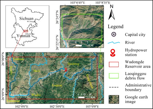
The Wudongde Reservoir area in the lower reaches of the Jinsha River is located at the junction of China’s Yunnan and Sichuan provinces. Influenced by historical upper tectonic activity and river erosion, a typical high mountain valley landscape has been formed (Zhang 2013; Zhao et al. 2018). The Jinsha River lies at the lowest elevation area at a valley depth between 800-2000 m. The peaks on both sides of the basin are approximately 2600 m above sea level, and there are folds and faults on both sides of the river, along with evidence of frequent geological disasters (Zhao et al. 2018). The climate of this region is characterized by a subtropical monsoon climate typical of a low latitude plateau. The region receives abundant sunshine, has high rates of evaporation, and is subjected to concentrated rainfall. The seasons alternate between wet and dry, with a rainy season from May to October. Peak rainfall occurs in July, and maximum daily rainfall is between 70 and 100 mm. The vegetation cover is dominated by natural savanna and sparse broad-leaved woods, and due to unreasonable logging and land reclamation, the natural vegetation has been severely damaged, resulting in a low vegetation cover (Zhang et al. 2011). The geological bodies are mainly sedimentary and metamorphic rocks (Li et al. 2014). The unique and complex topography, climate and geological characteristics of the study area have led to multiple geological hazards, such as landslides, collapses and debris flows. The water level fluctuations caused by human engineering activities, especially the construction of hydropower stations, have led to creep within the slopes of the upstream and downstream banks of the Wudongde Reservoir. This region is suitable for validating the performance of the SACTM baseline optimization TS-InSAR technique when used to identify creep.

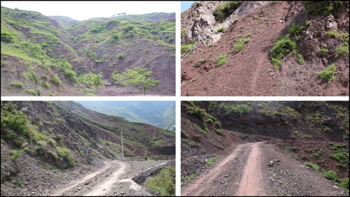
The Laoqinggou located on the east bank of the Xiaojiang River, a first-class tributary of the Jinsha River, is a small debris flow (He et al. 2003; Liu and Zhang 2004). Figure 2 shows some pictures of the material source area of the Laoqinggou debris flow. The field investigation found that the source area of the debris flow had loose soils, broken rocks and abundant accumulations of rock and soil after sliding, with obvious signs of creep.

Figure 2. Pictures of the Laoqinggou debris flow material source area.

2.2. HyP3 InSAR dataset

The SACTM interferometric baseline optimization TS-InSAR technique first requires obtaining the interferometric coherence coefficients and unwrapped interferograms. Nevertheless, the interferometric coherence coefficients and unwrapped interferograms can only be obtained after the interferometric processing of SAR images. Currently, conventional methods for interferometric processing that begin with SAR single-look complex (SLC) data require tremendous amounts of disk space, computational resources and processing time (Kennedy et al. 2021; Morishita et al. 2020), which makes it difficult to quickly obtain a large number of interferometric coherence coefficients and unwrapped interferograms. Fortunately, due to the open and free availability of large amounts of Sentinel-1 data and the development of big data cloud platform technologies, some online services can already provide a large amount of interferometric data for free with minimal wait times. These services include the LiCSAR system operated by COMET (Lazecky et al. 2020), the HyP3 system operated by NASA's Alaska Satellite Facility (ASF) (Kennedy et al. 2021), and the Advanced Rapid Imaging and Analysis (ARIA) system of NASA's Jet Propulsion Laboratory (JPL) (Bekaert et al. 2019). Among them, the HyP3 system can acquire interferometric pairs of arbitrary spatio-temporal baselines on demand and with a moderate pixel spacing (40 m) (https://asf.alaska.edu), which is convenient for coherence analysis and can help obtain better creep body identification results. Therefore, we used the interferometric data provided by HyP3 for interferometric baseline optimization and TS-InSAR processing.

HyP3 interferometric data are relatively easy to obtain, users can submit applications on the ASF portal or use the HyP3 Python SDK, and the system will automatically perform interferometric processing after data applications are submitted. Interferometric processing is performed using the GAMMA software hosted by Amazon Web Services (AWS). The processing steps consist mainly of data pre-processing, interferograms preparation and product creation (https://hyp3-docs.asf.alaska.edu). Notably, the process uses the Copernicus GLO-30 DEM to remove the topographic phase. The alignment accuracy of the interferometric pairs is better than 0.01 pixels. Adaptive spectral filtering and a mask with a coherence threshold of 0.1 is applied before phase unwrapping, which uses the minimum cost flow (MCF) method. The final available interferometric data contain wrapped and unwrapped interferograms, coherence maps, amplitude images, water mask images, DEMs, and look vector maps, etc. (https://hyp3.asf.alaska.edu/about).

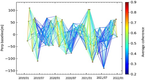
Theoretically, using all HyP3 interferometric data during the study time period could provide more alternatives for interferometric baseline optimization. However, as time increases, temporal decorrelation becomes significant, most low-coherence interferometric pairs become useless (Smittarello et al. 2022), and the creep bodies continue to deform. The creep deformation is likely to be larger than a quarter of the wavelength, i.e. 1.39 cm for Sentinel-1, which is prone to phase aliasing (Manconi et al. 2018; Moretto et al. 2017). To avoid introducing more error, this study sets the temporal baseline threshold as 108 days (encompassing three months) which can reflect the monthly variation in the coherence coefficients and provide a more relaxed alternative for interferometric baseline optimization. Due to the narrow orbit of the Sentinel-1 satellite system, satellites visit the same position repeatedly at close spatial distances (Prats-Iraola et al. 2015), which has little effect on the coherence (Braun 2021). Therefore, we do not set spatial baseline thresholds. Ultimately, we used the Baseline Tool of the HyP3 online service platform to obtain 725 descending track interferometric pairs over the time span from February 2019 to December 2021. Some of the HyP3 interferometric baseline information is shown in Table 1.

Table 1. Partial original HyP3 interferometric baseline information.

Interferometric pairs	Temporal baseline （day）	Spatial baseline （m）
20190209_20190221	12	81.4
20190209_20190305	24	136
20190209_20190329	48	27.2
20190209_20190410	60	−41.7
20190209_20190422	72	87.8
20190209_20190504	84	94.6
20190209_20190516	96	75
20190209_20190528	108	24.1
20190221_20190305	12	54.5
20190221_20190329	36	−54.3
20190221_20190410	48	−123.1
20190221_20190422	60	6.4
20190221_20190504	72	13.2
20190221_20190516	84	−6.5
20190221_20190528	96	−57.3
20190221_20190609	108	−164.2
20190305_20190329	24	−108.8
20190305_20190410	36	−177.6
20190305_20190422	48	−48.2
20190305_20190504	60	−41.3
20190305_20190516	72	−61
20190305_20190528	84	−111.8
20190305_20190609	96	−218.7
20190305_20190621	108	−164.5

3. Principle and methods

After obtaining the InSAR dataset from the HyP3 online service platform, the SACTM interferometric baseline optimization TS-InSAR technique needs to calculate the average coherence of each interferogram, distinguish the high coherence segment (high coherence months) and low coherence segment (low coherence months), calculate the average coherence of each segment separately, and then use the average coherence of each segment as a threshold to optimize the interferometric baselines. Finally, TS-InSAR processing is performed using the selected interferometric baselines to identify creep bodies. The overall technical flow is shown in Figure 3, which is mainly divided into interferogram segmentation, baseline optimization and TS-InSAR processing.

Figure 3. Flow chart of the processing sequence of the segmented average coherence threshold method (SACTM) using the interferometric baseline optimization TS-InSAR technique.

3.1. Interferogram segmentation

As shown in part 1 of Figure 3, the interferogram segmentation is based on the average coherences of all interferometric pairs (${\gamma }_{\mathit{all}}$) and monthly interferometric pairs (${\gamma }_{\mathit{month}}$). Additionally, this process separates the interferograms into high and low coherence segments by month. First, the coherence maps of all interferometric pairs are read, and then, based on the coherence maps, Eq. (1)(1) $${\gamma }_{\mathit{avg}}=\frac{\sum \begin{array}{c}W\\ i=1\end{array}\sum \begin{array}{c}I\\ j=1\end{array}{\gamma }_{(i,j)}}{W*I}$$(1) is used to calculate the average coherence of each interferogram in the study area (Wang et al. 2022). (1) $${\gamma }_{\mathit{avg}}=\frac{\sum \begin{array}{c}W\\ i=1\end{array}\sum \begin{array}{c}I\\ j=1\end{array}{\gamma }_{(i,j)}}{W*I}$$(1)

Where ${\gamma }_{\mathit{avg}}$ is the average coherence coefficient of the interferogram, $W$ and $I$ are the width and length of the image, respectively. $\gamma (i,j)$ is the coherence value at pixel $(i,j).$ ${\gamma }_{\mathit{avg}}$ range from 0.0 to 1.0, with 0.0 being completely no coherent and 1.0 being perfectly coherent.

After obtaining the average coherence coefficient of each interferogram in the study area, the average coherences of all interferometric pairs (${\gamma }_{\mathit{all}}$) can be calculated using Eq. (2)(2) $${\gamma }_{\mathit{all}}=\frac{\sum _{i=1}^n{\gamma }_{\mathit{avg}}}{n}$$(2) , and the monthly average coherence coefficient (${\gamma }_{\mathit{month}}$) can be calculated using Eq. (3)(3) $${\gamma }_{\mathit{month}}=\frac{\sum _{i=1}^m{\gamma }_{\mathit{avg}}}{m}$$(3) . Then, as shown in Eq. (4)(4) $$\{\begin{array}{c}{\gamma }_{\mathit{month}}\ge {\gamma }_{\mathit{all}},\text{high}\mathrm{ }\mathit{coherence}\mathrm{ }\mathit{segment}\\ {\gamma }_{\mathit{month}}<{\gamma }_{\mathit{all}},\mathit{low}\mathrm{ }\mathit{coherence}\mathrm{ }\mathit{segment}\end{array}$$(4) , the months with average coherence coefficients lower than the average coherences of all interferometric pairs are classified as low coherence segments (low coherence months), and the months with monthly average coherence coefficients higher than the average coherences of all interferometric pairs are classified as high coherence segments (high coherence months). (2) $${\gamma }_{\mathit{all}}=\frac{\sum _{i=1}^n{\gamma }_{\mathit{avg}}}{n}$$(2) (3) $${\gamma }_{\mathit{month}}=\frac{\sum _{i=1}^m{\gamma }_{\mathit{avg}}}{m}$$(3) (4) $$\{\begin{array}{c}{\gamma }_{\mathit{month}}\ge {\gamma }_{\mathit{all}},\text{high}\mathrm{ }\mathit{coherence}\mathrm{ }\mathit{segment}\\ {\gamma }_{\mathit{month}}<{\gamma }_{\mathit{all}},\mathit{low}\mathrm{ }\mathit{coherence}\mathrm{ }\mathit{segment}\end{array}$$(4)

Where $n$ is the number of all interferograms, ${\gamma }_{\mathit{all}}$ is their average coherence, $m$ is the number of interferograms per month and ${\gamma }_{\mathit{month}}$ is the monthly average coherence.

3.2. Baseline optimization

As shown in part 2 of Figure 3, baseline optimization is performed on the basis of the interferogram segmentation. The average coherence of all interferograms in the high coherence segment is defined as the high average coherence (${\gamma }_{\mathit{high}}$), the average coherence of all interferograms in the low coherence segment is defined as the low average coherence (${\gamma }_{\mathit{low}}$). Equations (5)(5) $${\gamma }_{\mathit{high}}=\frac{\sum _{\mathrm{i}=1}^H{\gamma }_{\mathit{avg}}}{H}$$(5) and (6)(6) $${\gamma }_{\mathit{low}}=\frac{\sum _{\mathrm{j}=1}^L{\gamma }_{\mathit{avg}}}{L}$$(6) , show how these values were derived. In the high coherence segment, ${\gamma }_{\mathit{high}}$ is used as the threshold to select the interferometric pairs. In the low coherence segment, ${\gamma }_{\mathit{low}}$ is used as the threshold to select the interferometric pairs. (5) $${\gamma }_{\mathit{high}}=\frac{\sum _{\mathrm{i}=1}^H{\gamma }_{\mathit{avg}}}{H}$$(5) (6) $${\gamma }_{\mathit{low}}=\frac{\sum _{\mathrm{j}=1}^L{\gamma }_{\mathit{avg}}}{L}$$(6)

Where $H$ is the number of all interferograms in the high coherence segment, ${\gamma }_{\mathit{high}}$ is the high average coherence, $L$ is the number of all interferograms in the low coherence segment, and ${\gamma }_{\mathit{low}}$ is the low average coherence coefficient.

3.3. TS-InSAR processing

After baseline optimization, the optimized interferometric pairs were processed using the TS-InSAR technique in the MintPy (The Miami insar timeseries software in Python) software package. MintPy is an open-source package for InSAR time series analysis and requires an input dataset that has already been unwrapped (https://mintpy.readthedocs.io). The InSAR dataset we downloaded from the HyP3 system has been unwrapped and can be directly analysed within the MintPy program. We only need to provide the path of the interferometric dataset, and MintPy can automatically read and perform the time series processing according to a predefined processing flow using parameter information. Finally, the three-dimensional (spatially two-dimensional and temporally one-dimensional) surface displacement can be obtained along the direction of the radar line of sight (LOS) (https://mintpy.readthedocs.io).

The default parameters and general processing steps that MintPy follows are described in detail in the literature (Yunjun et al. 2019). To ensure that TS-InSAR processing is performed using our optimized interferometric pairs, we turned off MintPy’s original network modification option. In addition, some parameters were changed to obtain more realistic creep deformation information within the study area, and the main processing steps and parameter information are as follows:

1. Load data: read the optimized HyP3 InSAR interferometric pairs.

2. Reference point determination: The reference point is the base point of all deformation data in the study area, and stable points in the regions with good coherence are generally selected. Since the study area is mostly mountainous, the coherence of most locations is highly variable. Therefore, in this study, the stable point was located on the Wudongde Dam and was manually selected as the reference point based on a priori knowledge.

3. Interferometric baseline network inversion: The network of interferograms can be converted into time series data using the weighted least square (WLS) estimator (Ansari et al. 2018) and by applying the inverse of covariance as the weights needed for the inversion process (Tough et al. 1995).

4. Tropospheric delay correction: Because of the large elevation differences in the study area, the empirical linear relationship between InSAR phase delay and elevation was used to correct for tropospheric delay (Doin et al. 2009).

5. Topographic residual correction: Corrects systematic topographic phase residuals caused by DEM errors.

6. Noise assessment: The root mean square error of the residual phase is calculated to assess the residual noise of the time series, and then the noisier data are removed (Lazecky et al. 2020).

7. Deformation rate estimation: Extraction of the final deformation rate and standard deviation of the deformation rate (Fattahi and Amelung 2015).

4. Results and discussion

4.1. Interferometric baseline optimization results

Once the 725 pairs of descending interferometric data for the study area are obtained from the HyP3 online service platform, the average coherence of each interferogram can be calculated according to Eq. (1)(1) $${\gamma }_{\mathit{avg}}=\frac{\sum \begin{array}{c}W\\ i=1\end{array}\sum \begin{array}{c}I\\ j=1\end{array}{\gamma }_{(i,j)}}{W*I}$$(1) . Figure 4 shows the interferometric baseline connection plots of all interferograms, and the colour of the baselines indicates the average coherence coefficient value. The average coherence coefficients in the study area have obvious monthly variations, with lower average coherence coefficients after July (blue baselines) and higher average coherence coefficients around January (red baselines), which is consistent with the alternating wet and dry climate in the study area.

Figure 4. Baseline connection diagram for all interferograms.

Figure 5 shows the average coherences of all interferometric pairs (${\gamma }_{\mathit{all}}$) and monthly interferometric pairs (${\gamma }_{\mathit{month}}$), and the average coherence for all interferometric pairs is 0.45. The months with average coherence coefficients higher than 0.45 (indicated by red triangles in the graph) are classified as high coherence segments. These were February, March, April, October, November and December in 2019; January, February, March, April, November and December in 2020; and January, February, March, November and December in 2021. The remaining months (indicated by blue triangles in the graph) are classified as low coherence segments. Then, according to Eqs. (3)(3) $${\gamma }_{\mathit{month}}=\frac{\sum _{i=1}^m{\gamma }_{\mathit{avg}}}{m}$$(3) and (4)(4) $$\{\begin{array}{c}{\gamma }_{\mathit{month}}\ge {\gamma }_{\mathit{all}},\text{high}\mathrm{ }\mathit{coherence}\mathrm{ }\mathit{segment}\\ {\gamma }_{\mathit{month}}<{\gamma }_{\mathit{all}},\mathit{low}\mathrm{ }\mathit{coherence}\mathrm{ }\mathit{segment}\end{array}$$(4) , the high average coherence coefficient is 0.51, and the low average coherence coefficient is 0.39. In the high coherence segment, we eliminate the interferometric pairs with coherence coefficients less than 0.51; in the low coherence segment. The interferometric pairs with coherence less than 0.39 are removed. The 295 interferometric pairs left are the final optimized interferometric pairs, and the information for the optimized partial interferograms is shown in Table 2.

Figure 5. The average coherences of all interferometric pairs and monthly interferometric pairs.

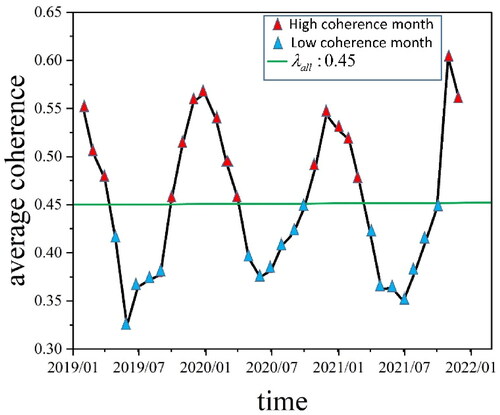
Table 2. Partial interferograms information after baseline optimization.

Interferometric pairs	Temporal baseline （day）	Average coherence
20190209_20190221	12	0.7295
20190209_20190305	24	0.59
20190209_20190329	48	0.6221
20190209_20190410	60	0.5818
20190221_20190305	12	0.7442
20190221_20190329	36	0.6517
20190221_20190410	48	0.5658
20190221_20190422	60	0.5879
20190221_20190504	72	0.5373
20190221_20190516	84	0.5403
20190305_20190329	24	0.615
20190305_20190410	36	0.535
20190305_20190422	48	0.5436
20190305_20190504	60	0.5341

4.2. Creep body identification results

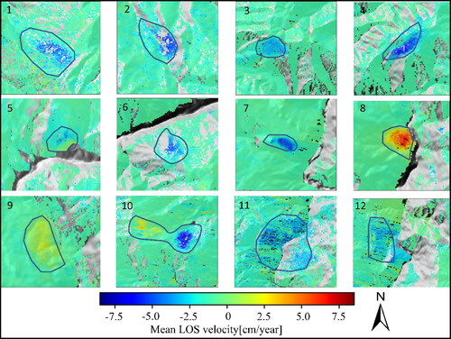
Using the TS-InSAR method in Section 3.3, we performed time series processing for the optimized HyP3 InSAR interferometric dataset, as shown in Figure 6, and successfully obtained the annual average deformation rate in the descending LOS direction from February 2019 to 2022. Positive deformation rate values indicate movement towards the sensor, while negative values indicate movement away from the sensor. There are several creep regions in the study area with significant deformation rates in the descending LOS direction, indicated by the numbers 1 to 12, and their detailed deformation information are shown in Figure 7. We reviewed historical data and found that these creep regions match with historical geologic hazard locations: No. 5 is the location of Zaogutian dangerous rock body, No. 7 is the Shuanglongtan landslide, No. 8 is the Dapingdi landslide, No. 9 is the Dacun-Fujiapingzi landslide, and No. 10 is the Lannigou landslide. The remaining creep bodies also match hazard areas identified in the existing literature (Ren et al. 2022; Wang et al. 2013; Xie et al. 2016; Zhao et al. 2018), which indicates that the creep body identification results from this study are reliable.

Figure 6. The LOS direction annual average deformation rate. The black curve symbol indicates the approximate area of significant creep.

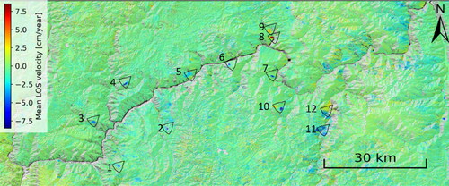
Figure 7. Enlarged view of the significant creep areas marked in Figure 6.

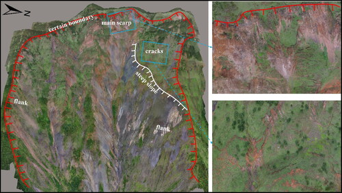
We have investigated the Shuanglongtan landslide and the landslide source area of Lannigou in the field. Figure 8 shows the unmanned aerial vehicle (UAV) realistic three-dimensional model of the Shuanglongtan landslide. From this model, it can be seen obvious landslide boundary, main scarp, minor scarp, clastic material and erosion valley. The sliding rock and soil were washed by the running water, forming a fan-shaped deposit at the bottom of the landslide body, which indicates that the landslide body is in a long-term sliding state. Figure 9 shows the UAV realistic three-dimensional model obtained in the source area of the Lannigou landslide. It can be seen the obvious landslide morphology, boundary, flanks, cracks, main scarp and other landslide features are obvious.

Figure 8. UAV realistic three-dimensional model of the Shuanglongtan landslide. The red serrated line is the certain boundary and the white serrated line indicates the steep slope.

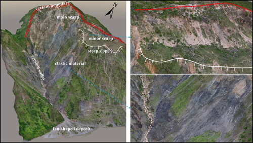
Figure 9. UAV realistic three-dimensional model of the Lannigou landslide source area.

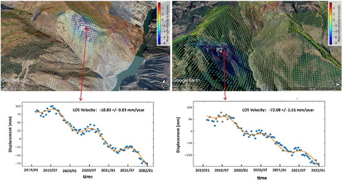
To further analyse the creep characteristics, two feature points (P1 and P2 in Figure 10) were selected from the Shuanglongtan landslide and the Lannigou landslide to extract their time series deformation curves. The lower part of Figure 10 shows the time series deformation curves of points P1 and P2, from which we can see that curves contain obvious seasonal fluctuations. It is presumed that creep is mainly caused by rainfall and weathering, and the alternating wet and dry climate of the creep area and the high slope of the terrain are conducive to the development of fissures. During the six month long dry season, the rock and soil lose water, and the cohesive force of the material is reduced to a minimum. This loose state makes it harder for the rock and sediment to withstand the force of gravity. In the rainy season, the infiltration of water causes the rock and soil to become heavier, while the moisture simultaneously reduces the friction along the sliding surface. This is especially true when heavy rain occurs, which is when the creep body is most prone to rapid destabilization, ultimately forming a geological disaster.

Figure 10. Creep areas and characteristic points P1 and P2. The points indicate the locations of the time–displacement curves of the Shuanglongtan landslide (left) and Lannigou landslide (right). The background is from Google Earth.

4.3. Baseline optimization assessment

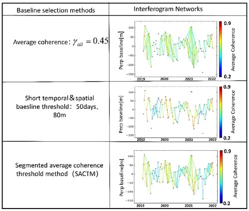
To assess the performance of the interferometric baseline optimization method, we compare it with two conventional interferometric baseline selection methods, the average coherence threshold and the short spatio-temporal baseline thresholds, which do not take into account the difference in coherence months. The final evaluation results are achieved by analysing the interferometric network structure and the standard deviation of the deformation rate.

The three Interferometric baseline networks in Figure 11 are obtained using the average coherence threshold (0.45), the short spatio-temporal baseline thresholds (50 days for the temporal baseline and 80 meters for the spatial baseline) and the SACTM method presented in this paper. It can be seen from the figure that the use of the short spatio-temporal baseline thresholds cannot eliminate the interferometric pairs that have short intervals but poor coherence (blue baseline). Additionally, the figure shows that there are few interferometric pairs connected to each scene SAR image, which easily introduces the decorrelation error. Using the average coherence as the threshold improves the overall coherence, but the interferometric network shows redundant interferometric pairs during the dry season, sparse interferometric pairs in the rainy season, and three disconnections, despite the rainy season often being a creep-prone period. Additionally, the absence of key SAR data can lead to a significant reduction in time series inversion accuracy. In contrast, the interferometric baselines optimized by the SACTM method can reduce the redundancy of interferometric pairs during high coherence months and increase the number of interferometric pairs in low coherence months while improving the overall coherence. This is done without interferometric baseline disconnections, which ultimately results in a more robust interferometric baseline network.

Figure 11. Different methods and corresponding baseline connection diagrams.

The standard deviation of the deformation rate can be used to characterize the noise level of the InSAR time series (Mengyao et al. 2021; Murray et al. 2019), with higher values indicating a noisier deformation rate map, which can be calculated using Eq. (7) (Mengyao et al. (7) $$\{\begin{array}{c}\sigma =\sqrt{\frac{1}{M}\sum _{i=1}^M\left(V_i-\mu \right)}\\ \mu =\frac{1}{M}\sum _{i=1}^M{V}_i\end{array}$$(7) 2021). (7) $$\{\begin{array}{c}\sigma =\sqrt{\frac{1}{M}\sum _{i=1}^M\left(V_i-\mu \right)}\\ \mu =\frac{1}{M}\sum _{i=1}^M{V}_i\end{array}$$(7)

Where $\sigma$ is the standard deviation, $M$ is the number of pixels, and $V_i$ is the deformation rate of the i-th pixel.

The standard deviations of the deformation rates obtained from TS-InSAR analysis using SACTM, the average coherence and the short spatio-temporal baseline thresholds are 0.61, 0.92 and 0.81, respectively. SACTM takes into account the different coherence values each month and can obtain smaller standard deviations for the deformation rates, which means that the error is smaller and the overall deformation rate is more stable.

4.4. Case study of Laoqinggou

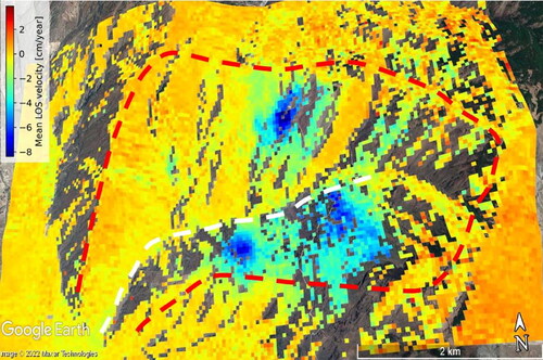
The Laoqinggou debris flow is taken as a case study to verify the applicability of the SACTM-based interferometric baseline optimization TS-InSAR technique in different scenarios. In the Laoqinggou debris flow region, a total of 710 pairs of descending HyP3 InSAR interferometric pairs from February 2019 to 2022 were obtained, and the average coherence (0.50) of all interferograms was calculated, the months with average coherence values higher than 0.50 were February, March, April, October, November, and December in 2019; January, February, March, October, November, and December in 2020; and January, February, March, November, and December in 2021. These months are classified as the high coherence segment, and the remaining months are classified as the low coherence segment. The high average coherence is 0.59, and the low average coherence is 0.43. A total of 302 pairs of interferometric images were acquired by the SACTM baseline optimization method for TS-InSAR processing. The identified creep areas are shown in Figure 12. The identified creep areas are mainly distributed on both sides of the debris flow gully which shows very clear signs of slipping.

Figure 12. Annual average LOS velocity of the Laoqinggou debris flow region, the white dashed line is the debris flow gully, and the red dashed line is the debris flow boundary.

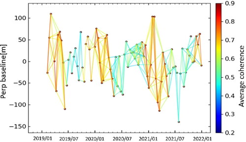
The interferometric baseline in the Laoqinggou debris flow region is selected by the SACTM method, as shown in Figure 13. Similar to the results of the Wudongde Reservoir Area, the SACTM method presented in this paper can select a robust interferometric baseline network. The standard deviation of the deformation rates obtained from the TS-InSAR analysis with the SACTM threshold, the average coherence and the short spatio-temporal baselines are 0.82, 0.96 and 1.00, respectively. The SACTM method can obtain a smaller standard deviation for the deformation rate, which indicates that the interferometric baseline method in this paper is also applicable in the Laoqinggou debris flow region.

Figure 13. Schematic of the optimized interference baseline network in the Laoqinggou debris flow region.

5. Conclusion

The TS-InSAR technique plays an important role in creep body identification. To address the limitations of conventional TS-InSAR using short spatio-temporal baselines or a fixed average coherence threshold to select interferometric pairs, this paper proposes the SACTM method to optimize the interferometric baselines. Compared with the traditional interferometric pair selection methods, this method takes into account the monthly coherence variability, which can improve the overall coherence of observations from the Wudongde Reservoir area. Additionally, this method reduces the redundancy of interferometric pairs during high coherence months, increases the number of interferometric pairs in low coherence months, and obtains a more robust interferometric baseline network. TS-InSAR processing using the interferometric pairs optimized by the SACTM method effectively identifies creep bodies in the Wudongde Reservoir area. The standard deviation of the deformation rate is 0.67, which is smaller than the standard deviation obtained by the average coherence threshold and the threshold methods that use short spatio-temporal baselines, this indicates that the introduced error is smaller. Finally, a case study was conducted in the Laoqinggou debris flow region, significant creep deformation information was found, and a smaller standard deviation for the deformation rate was obtained, which proved the applicability of the proposed method.

Disclosure statement

No potential conflict of interest was reported by the authors.

Data availability statement

The authors confirm that the data supporting the findings of this study are available within the article.

Additional information

Funding

This research was funded by the National Natural Science Foundation of China (No. 41961061) and the Yunnan Fundamental Research Projects (NO. 202001AT070057) and ‘Revitalizing Yunnan Talents Support Program’ project (No.YNWR-QNBJ-2020-048) and Yunnan Academician and Expert Workstation (No.2017IC063)

References

- Ansari H, De Zan F, Bamler R. 2018. Efficient phase estimation for interferogram stacks. IEEE Trans Geosci Remote Sens. 56(7):4109–4125. 10.1109/tgrs.2018.2826045.
- Ansari H, De Zan F, Parizzi A. 2021. Study of systematic bias in measuring surface deformation with SAR interferometry. IEEE Trans Geosci Remote Sens. 59(2):1285–1301. 10.1109/tgrs.2020.3003421.
- Baran I, Stewart M, Claessens S. 2005. A new functional model for determining minimum and maximum detectable deformation gradient resolved by satellite radar interferometry. IEEE Trans Geosci Remote Sens. 43(4):675–682. 10.1109/tgrs.2004.843187.
- Bekaert DP, Karim M, Linick JP, Hua H, Sangha S, Lucas M, Malarout N, Agram PS, Pan L, Owen SE. 2019. Development of open-access standardized InSAR displacement products by the advanced rapid imaging and analysis (ARIA) project for natural hazards. In AGU Fall Meeting Abstracts. Vol. 2019, pp. G23A–04.
- Braun A. 2021. Retrieval of digital elevation models from Sentinel-1 radar data – open applications, techniques, and limitations. Open Geosci. 13(1):532–569. 10.1515/geo-2020-0246.
- Cigna F, Tapete D. 2021. Present-day land subsidence rates, surface faulting hazard and risk in Mexico City with 2014–2020 Sentinel-1 IW InSAR. Remote Sens Environ. 253: 112161. 10.1016/j.rse.2020.
- Crosta GB, Frattini P, Agliardi F. 2013. Deep seated gravitational slope deformations in the European Alps. Tectonophysics. 605:13–33. 10.1016/j.tecto.2013.04.028.
- Doin MP, Lasserre C, Peltzer G, Cavalie O, Doubre C. 2009. Corrections of stratified tropospheric delays in SAR interferometry: validation with global atmospheric models. J Appl Geophys. 69(1):35–50. 10.1016/j.jappgeo.2009.03.010.
- Du J-C, Teng H-C. 2007. 3D laser scanning and GPS technology for landslide earthwork volume estimation. Autom Constr. 16(5):657–663. 10.1016/j.autcon.2006.11.002.
- Fattahi H, Amelung F. 2015. InSAR bias and uncertainty due to the systematic and stochastic tropospheric delay. J Geophys Res Solid Earth. 120(12):8758–8773., 10.1002/2015jb012419.
- He YP, Xie H, Cui P, Wei FQ, Zhong DL, Gardner JS. 2003. GIS-based hazard mapping and zonation of debris flows in Xiaojiang Basin, southwestern China. Environ Geol. 45(2):286–293. 10.1007/s00254-003-0884-0.
- Howard HR, Manandhar S, Wang Q, McMillan JM, Qie G, Liu X, Thapa K, Xu X, Wang G. 2022. Spatially characterizing land surface deformation and permafrost active layer thickness for Donnelly installation of Alaska using DInSAR and MODIS data. Cold Reg Sci Technol. 196:103510. 10.1016/j.coldregions.2022.103510.
- Kang Y, Lu Z, Zhao C, Xu Y, Kim J-w, Gallegos AJ. 2021. InSAR monitoring of creeping landslides in mountainous regions: a case study in Eldorado National Forest, California. Remote Sens Environ. 258:112400. 10.1016/j.rse.2021.112400.
- Kang Y, Lu Z, Zhao C, Zhang Q, Kim J-W, Niu Y. 2019. Diagnosis of Xinmo (China) landslide based on interferometric synthetic aperture radar observation and modeling. Remote Sens. 11(16):1846. 10.3390/rs11161846.
- Kang Y, Zhao C, Zhang Q, Lu Z, Li B. 2017. Application of InSAR techniques to an analysis of the Guanling landslide. Remote Sens. 9(10):1046. 10.3390/rs9101046.
- Kennedy J, Anderson R, Biessel R, Chase T, Ellis O, Fairbanks K, Fleming C, Horn W, Johnston A, Kristenson H. 2021. Skip the processing: on demand analysis-ready InSAR from ASF. AGU Fall Meeting Abstracts (Vol. 2021, p. G45B-0395).
- Lanari R, Mora O, Manunta M, Mallorqui JJ, Berardino P, Sansosti E. 2004. A small-baseline approach for investigating deformations on full-resolution differential SAR interferograms. IEEE Trans Geosci Remote Sens. 42(7):1377–1386. 10.1109/tgrs.2004.828196.
- Lauknes TR, Zebker HA, Larsen Y. 2011. InSAR deformation time series using an L-1-norm small-baseline approach. IEEE Trans Geosci Remote Sens. 49(1):536–546. 10.1109/tgrs.2010.2051951.
- Lazecky M, Spaans K, Gonzalez PJ, Maghsoudi Y, Morishita Y, Albino F, Elliott J, Greenall N, Hatton E, Hooper A, et al. 2020. LiCSAR: an automatic InSAR tool for measuring and monitoring tectonic and volcanic activity. Remote Sens. 12(15):2430. 10.3390/rs12152430.
- Li H, Hao W, Pan Y, Yang J, Xiao Y, Xie S. 2014. Composition and structure of geological prospecting in river deep overburden layers at dam site of Wudongde Hydropower Station. J. Eng. Geol. 22(5):944–950.
- Liu XL, Zhang D. 2004. Comparison of two empirical models for gully-specific debris flow hazard assessment in Xiaojiang valley of southwestern China. Nat Hazards. 31(1):157–175. 10.1023/B:NHAZ.0000020274.54664.a0.
- Lopez-Quiroz P, Doin M-P, Tupin F, Briole P, Nicolas J-M. 2009. Time series analysis of Mexico City subsidence constrained by radar interferometry. J Appl Geophys. 69(1):1–15. 10.1016/j.jappgeo.2009.02.006.
- Manconi A, Kourkouli P, Caduff R, Strozzi T, Loew S. 2018. Monitoring surface deformation over a failing rock slope with the ESA sentinels: insights from Moosfluh instability, Swiss Alps. Remote Sen. 10(5):672. 10.3390/rs10050672.
- Mengyao GAO, Caijun XU, Yang LIU. 2021. Evaluation of time‑series InSAR tropospheric delay correction methods over north‑western margin of the Qinghai‑Tibet Plateau. Geomat Inf Sci Wuhan Univ. 46(10):1548–1559.
- Mohammadimanesh F, Salehi B, Mahdianpari M, English J, Chamberland J, Alasset P-J. 2019. Monitoring surface changes in discontinuous permafrost terrain using small baseline SAR interferometry, object-based classification, and geological features: a case study from Mayo, Yukon Territory, Canada. GIscience Remote Sens. 56(4):485–510. 10.1080/15481603.2018.1513444.
- Moretto S, Bozzano F, Esposito C, Mazzanti P, Rocca AJG. 2017. Assessment of landslide pre-failure monitoring and forecasting using satellite SAR interferometry. Geosciences. 7(2):36.
- Morishita Y, Lazecky M, Wright TJ, Weiss JR, Elliott JR, Hooper A. 2020. LiCSBAS: an open-source InSAR time series analysis package integrated with the LiCSAR automated sentinel-1 InSAR processor. Remote Sens. 12(3):424. 10.3390/rs12030424.
- Murray KD, Bekaert DPS, Lohman RB. 2019. Tropospheric corrections for InSAR: statistical assessments and applications to the Central United States and Mexico. Remote Sens Environ. 232:111326. 10.1016/j.rse.2019.111326.
- Nichol J, Wong MS. 2005. Detection and interpretation of landslides using satellite images. Land Degrad Dev. 16(3):243–255. 10.1002/ldr.648.
- Prats-Iraola P, Rodriguez-Cassola M, De Zan F, Scheiber R, Lopez-Dekker P, Barat I, Geudtner D. 2015. Role of the orbital tube in interferometric spaceborne SAR missions. IEEE Geosci Remote Sensing Lett. 12(7):1486–1490. 10.1109/lgrs.2015.2409885.
- Ren K, Yao X, Li R, Zhou Z, Yao C, Jiang S. 2022. 3D displacement and deformation mechanism of deep-seated gravitational slope deformation revealed by InSAR: a case study in Wudongde Reservoir, Jinsha River. Landslides. 19(9):2159–2175. 10.1007/s10346-022-01905-8.
- Santoro M, Wegmuller U, Askne JIH. 2010. Signatures of ERS-envisat interferometric SAR coherence and phase of short vegetation: an analysis in the case of maize fields. IEEE Trans Geosci Remote Sens. 48(4):1702–1713., 10.1109/tgrs.2009.2034257.
- Smittarello D, d’Oreye N, Jaspard M, Derauw D, Samsonov S. 2022. Pair selection optimization for InSAR time series processing. J Geophys Res: Solid Earth. 127 e2021JB022825
- Sui L, Wang X, Zhao D. 2008. Application of 3D laser scanner for monitoring of landslide hazards. Int Arch Photogramm Remote Sens Spat Inf Sci. 37(PART B1).
- Sun N, Wang Y. 2018. Analysis of land subsidence monitoring in a mining area with time series InSAR technology, Proceedings ISPRS Symposium. Int Arch Photogramm Remote Sens Spatial Inf Sci. XLII-3:1589–1595.
- Tough J, Blacknell D, Quegan SJP. 1995. A statistical description of polarimetric and interferometric synthetic aperture radar data. Proc R Soc Lond, A: Math Phys Sci. 449: 567–589.
- Wang ZH, Guo DH, Zheng XW, Wang JC, Guo ZC, Dong LN. 2011. Remote sensing interpretation on June 28, 2010 Guanling landslide, Guizhou Province, China. Geosci. Front. 18:310–316.
- Wang G, Xie M, Chai X, Wang L, Dong C. 2013. D-InSAR-based landslide location and monitoring at Wudongde hydropower reservoir in China. Environ Earth Sci. 69(8):2763–2777. 10.1007/s12665-012-2097-x.
- Wang S, Zhang G, Chen Z, Cui H, Zheng Y, Xu Z, Li Q. 2022. Surface deformation extraction from small baseline subset synthetic aperture radar interferometry (SBAS-InSAR) using coherence-optimized baseline combinations. GIscience Remote Sens. 59(1):295–309. 10.1080/15481603.2022.2026639.
- Xie M, Huang J, Wang L, Huang J, Wang Z. 2016. Early landslide detection based on D-InSAR technique at the Wudongde hydropower reservoir. Environ Earth Sci. 75(8):1–13. 10.1007/s12665-016-5446-3.
- Xu Q, Guo C, Dong X, Li W, Lu H, Fu H, Liu X. 2021a. Mapping and characterizing displacements of landslides with InSAR and airborne LiDAR technologies: a case study of Danba County, Southwest China. Remote Sens. 13(21):4234. 10.3390/rs13214234.
- Xu Y, Schulz WH, Lu Z, Kim J, Baxstrom K. 2022. Geologic controls of slow-moving landslides near the US West Coast (vol 18, pg 3353, 2021). Landslides. 19(2):537–537. 10.1007/s10346-021-01801-7.
- Yunjun Z, Fattahi H, Amelung F., 2019. Small baseline InSAR time series analysis: unwrapping error correction and noise reduction. Comput Geosci. 133:104331.
- Zhang W, Li H-Z, Chen J-p, Zhang C, Xu L-m, Sang W-f 2011. Comprehensive hazard assessment and protection of debris flows along Jinsha River close to the Wudongde dam site in China. Nat Hazards. 58(1):459–477. 10.1007/s11069-010-9680-9.
- Zhang Y, Meng XM, Dijkstra TA, Jordan CJ, Chen G, Zeng RQ, Novellino A. 2020. Forecasting the magnitude of potential landslides based on InSAR techniques. Remote Sens Environ. 241:111738. 10.1016/j.rse.2020.111738.
- Zhang QY, Xiang W, Li XJ. 2007. Application of nondestructive detecting technology for geological radar in a large-scale highway lanslide treatment. KEM. 353-358:2309–2312.
- Zhang W. 2013, June 1. Research of evaluation methods for rock mass structures in the Wudongde Hydropower Reservoir Region [Ph.D. thesis]. Changchun, China: Jilin University.
- Zhao C, Kang Y, Zhang Q, Lu Z, Li B. 2018. Landslide identification and monitoring along the Jinsha River catchment (Wudongde Reservoir Area), China, using the InSAR method. Remote Sens. 10(7):993. 10.3390/rs10070993.
- Zhao C, Lu Z, Zhang Q, de la Fuente J. 2012. Large-area landslide detection and monitoring with ALOS/PALSAR imagery data over Northern California and Southern Oregon, USA. Remote Sens Environ. 124:348–359. 10.1016/j.rse.2012.05.025.
- Zhu Y, Qiu H, Yang D, Liu Z, Ma S, Pei Y, He J, Du C, Sun H. 2021. Pre- and post-failure spatiotemporal evolution of loess landslides: a case study of the Jiangou landslide in Ledu, China. Landslides. 18(10):3475–3484. 10.1007/s10346-021-01714-5.