Total organic carbon estimation in seagrass beds in Tauranga Harbour, New Zealand using multi-sensors imagery and grey wolf optimization

Abstract

Estimation of carbon stock in seagrass meadows is in challenges of paucity of assessment and low accuracy of the estimates. In this study, we used a fusion of the synthetic aperture radar (SAR) Sentinel-1 (S-1), the multi-spectral Sentinel-2 (S-2), and coupled this with advanced machine learning (ML) models and meta-heuristic optimization to improve the estimation of total organic carbon (TOC) stock in the Zostera muelleri meadows in Tauranga Harbour, New Zealand. Five scenarios containing combinations of data, ML models (Random Forest, Extreme Gradient Boost, Rotation Forest, CatBoost) and optimization were developed and evaluated for TOC retrieval. Results indicate a fusion of S1, S2 images, a novel ML model CatBoost and the grey wolf optimization algorithm (the CB-GWO model) yielded the best prediction of seagrass TOC (R², RMSE were 0.738 and 10.64 Mg C ha⁻¹). Our results provide novel ideas of deriving a low-cost, scalable and reliable estimates of seagrass TOC globally.

Keywords:

• Seagrass
• total organic carbon
• Sentinel image
• CatBoost
• metaheuristic optimization

1. Introduction

Seagrass meadows are hotspots of biodiversity (Mari et al. 2021; McHenry et al. 2021) and are widely distributed in different climatic regions. In recent years, diverse research approaches have unveiled valuable seagrass ecosystem services of nursery and breeding ground (Jiang et al. 2020), water filtration (Bulmer et al. 2018; Lincoln et al. 2021), food supplies (Jankowska et al. 2019), coastal stabilization (James et al. 2020) and sediment trapping (Nordlund et al. 2016; Potouroglou et al. 2017; Orth et al. 2020).

Since 2012, the blue carbon initiative (Fourqurean et al. 2012) has emerged in respond to the climate change emergency and the essential requirement of greenhouse gas (GHG) reduction (Hilmi et al. 2021). According to the Intergovernmental Panel on Climate Change (IPCC), a reduction of global GHG emission to 4–10% to the year 2030 will help to alleviate the negative impact of global warming (Grubb et al. 2022). Aside from a direct reduction of GHG from production sectors in the countries worldwide, absorption and sequestration of CO₂ emission in the atmosphere is crucial to reach and complete the 13th Sustainable Development Goal (SDG). Among coastal ecosystem, seagrass has been identified as the role in the sequestration of carbon sources (Duarte et al. 2013; Macreadie et al. 2019; Bedulli et al. 2020; Stankovic et al. 2021), through its potential to absorb and store the CO₂ in deep soil layers. There are arguments that restoration and enhancement of seagrass-based ecosystems are a potential candidate for a long-term, nature-based solution to climate change mitigation and adaptation (Stankovic et al. 2021), though the extent to which this is possible is challenged, with the IPCC suggesting that coastal blue carbon systems can sequester only about 0.5% of present day emissions (IPCC 2019). A major gap in the evaluation of the potential significance of seagrass meadow blue carbon is the limited number of assessment of carbon stock, which challenges any understanding of the relationship between seagrass and climate change mitigation (Thorhaug et al. 2017; Salinas et al. 2020).

To measure carbon stock in a seagrass meadow, field sampling coupled with laboratory analysis is the classical approach (Howard et al. 2014; Susi et al. 2019). This traditional sampling and soil analysis can provide an accurate measurement of total carbon stock; however a number of drawbacks remains, associated with the high person-time requirement that normally results in small-scale observations at a few, readily accessible locations. Remotely based approaches using the satellite-borne remote sensing and development of models are emerging as the fastest route to large-scale, long-term and cost effective mapping and monitoring of carbon stock (Pham et al. 2019; Sani et al. 2019). Unlike the mapping of seagrass biomass or above-ground parameters, which are potentially derived directly from remotely sensed reflectance (Ha et al. 2021a), a carbon stock retrieval that includes sediment contribution often requires an indirect estimation approach through the using of spectral index, soil index, and a variety of types of remote sensing band (Yang et al. 2015; Sani et al. 2019; Pham et al. 2021). As a result, the fusion of both multi-spectral data, returning visible and infra-red optical information, with synthetic aperture radar (SAR) data, returning information on texture and roughness, have been preferred recently (Yang and Guo 2019; Le et al. 2021; Nguyen et al. 2022). This has motivated a wide application of the Sentinel family of remote sensing satellites, with the most popular sensors being the SAR-equipped Sentinel-1 (S-1) and the multi-spectral Sentinel-2 (S-2). S-1 acquires the image at a spatial resolution of roughly 23.5 m, with 12-day revisiting cycle, and collects data at two polarizations as vertical transmission-horizontal receive (VH) and vertical transmission-vertical receive (VV) (ESA-S1 2020). S-2 provides 12 spectral bands (visible-near infrared (VNIR) to short wavelength infrared (SWIR)) at spatial resolutions of 10–60 m, on a 5-day revisit cycle (Naud et al. 2021). The integration of S-1 and S-2 sensors has been employed for retrieval of various biophysical parameters (Mahdianpari et al. 2018; Navarro et al. 2019; Le et al. 2021; Ha et al. 2021a), however their potential use for seagrass carbon stock estimation, is still in its infancy and requires further experiments to validate the sensor performance (Macreadie et al. 2019; Sani et al. 2019).

In order to accurately estimate the carbon stock from satellite imagery, a retrieval model, which helps to quantify the relationship between remote sensing and field measured data is a central component. Currently, machine learning (ML) models are widely used in developing these relationships. ML is capable of dealing with non-linear relationship, learning from a variety of data types, and has recently contributed to a high success of biophysical appraisal (Muttil and Chau 2007; Lary et al. 2016; Ahmad, 2019). More recently, the use of metaheuristic optimization for feature selection is emerging as the tool of choice for feature reduction to improve the quality of retrieval modelling (Agrawal et al. 2021; Ezenkwu et al. 2021; Ha et al. 2021a). To our best knowledge, a fusion of satellite products, ML modelling and metaheuristic optimization has yet to be evaluated for prediction of any seagrass ecosystem attributes.

In this study, we develop such an approach, using the fusion of S-1, S-2 datasets, the state-of-the-art ML model (CatBoost (CB)) and the grey wolf optimization (GWO), to estimate, for the first time, the seagrass total organic soil carbon stock at an accuracy of R² 0.74 in Tauranga Harbour, New Zealand. The method contributes reliable and advanced techniques as a low cost, accurate estimator of seagrass carbon stock that with appropriate validation and calibration could be applied worldwide.

2. Material and methodology

2.1. Study site

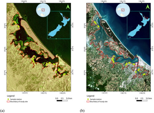
Our study site is Tauranga Harbour, which located in the western part of the Bay of Plenty, North Island, New Zealand (Ellis and Cawthron 2013) with approximately 14,000 ha of water surface area at high tide. The harbour (Figure 1) comprises north and south basins that drain in different directions to the Bay of Plenty marine environment. There are six sub-estuarines in the northern and southern basin. Two basins are connected through a intertidal flat in the central of the harbour (Tay et al. 2013). Seagrass meadows in Tauranga Harbour are in long-term decline (Ha et al. 2021b) but persists despite anthropogenic pressures from New Zealand’s busiest port, intensive catchment agriculture, and ongoing urban development (Tay et al. 2013; Cussioli et al. 2019; Figure 1). Only one small-leaved seagrass species has been recorded in the study area, Zostera muelleri (Tara et al. 2019), and mostly occupies in the inter-tidal region (Park 1999; Ha et al. 2020). The tide is semi-diurnal at a tidal range of 0.5–2 m (Reeve et al. 2018). At low tide, seagrass is mostly exposed to the air and hence is available for S-1 and S-2 imaging. The soil around the harbour was classified as saline grey raw soils with the loam covering the sand and 0–2% clay in the topsoil (Environment Bay of Plenty 2010). The depth of root penetration ranges between 20 and 60 cm (Environment Bay of Plenty 2010) from the soil surface, and therefore there is potential for seagrass meadows to contribute to carbon sequestration.

Figure 1. Study site – Tauranga Harbour in the illustration of (a) Sentinel-1 (date of acquisition 31 March 2020, pseudo colour using the combination of VH-VV-VH); (b) Sentinel-2 (date of acquisition 5 April 2020, pseudo colour using the combination of ρ_Red–ρ_Green–ρ_Blue) and the ground truth points during the field survey.

2.2. Material

2.2.1. Satellite image acquisition

S-1 and S-2 scenes were retrieved from the European Space Agency (ESA) Copernicus hub (https://scihub.copernicus.eu/dhus/#/home) and the United States geological survey (USGS) global visualization viewer (USGS GloVIS, https://glovis.usgs.gov/) (Table 1). The S-1 image was originally processed to level 1 and projected to the World Geodetic System (WGS-84) while the S-2 image was in level 1 C and the WGS-84 Universal Transverse Mercator (UTM), zone 60 south (60S), respectively. The images acquired on 31 March (for S-1) and 5 April (for S-2 images) were selected as closest to the field surveys 7–25 March 2020 and coincident with low tide to have a chance of exposing most seagrass meadows in the harbour (Ha et al. 2020, 2021a).

Table 1. Acquisitions of Sentinel-1 and Sentinel-2 datasets.

Sensor	Scene processing	Selected band	Acquisition date	Acquisition time	Local low tide
Sentinel-1	Ground range detected (GRD) level 1, sensor mode: interferometric wide swath (IW)	Dual-polarimetric VH, VV	31 March 2020	19:07	19:02
Sentinel-2	Level 1 C	Band 1 to 8, 8 A vegetation (8 A-V), 11, 12	5 April 2020	10:15	10:17

2.2.2. Field data collection

The field survey was conducted in the austral summer (between 7th and 25th March 2020). The locations of the soil sampling plots were randomly selected from ground truth points (GTPs) data collected in 2019 (Ha et al. 2020) with the additional requirement of accessibility with sampling equipment. At low tide at each site, we designated a 10 m × 10 m plot inside the seagrass meadow, which fitted a pixel size of the satellite image and collected one soil core at the centre of the plot using a rigid plastic soil corer with a metal cutting tip. A total of 57 sediment samples to the depth of 50 cm were collected (Howard et al. 2014). Soil subsamples (a maximum of 20 cm³ in volume) were extracted using a plastic syringe from each of sampling three depths (10, 30, 50 cm), and kept in labelled plastic bags, and maintained at −10 °C until further sample processing in the laboratory (Saiz and Albrecht 2016; Smith et al. 2020).

2.3. Methodology

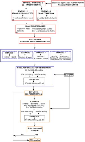
To estimate the seagrass meadow TOC from remotely sensed data, we developed our novel method using a series of steps (Figure 2): Preprocessing and creating of S-1 and S-2 stacked images, was followed by testing the performance of four different ML models described below for TOC retrieval through four scenarios, described below, using the field data for training and validation of models. Scenario 1 used only S-1 data. Scenario 2 used only S-2 data. Scenario 3 used both S-1 and S-2 data, and Scenario 4 was based on Scenario 3 but with the addition of feature selection using correlation, described below. After the ML model best predicting TOC was selected, Scenario 5 was run which used both S-1 and S-2 data and feature selection with the GWO algorithm.

Figure 2. Flowchart of the research with codes of red (image processing), blue (retrieval of the TOC using scenario 1–scenario 4) and orange (retrieval of the TOC using Scenario 5) colours.

2.3.1. Soil samples analysis and total organic carbon measurement

Soil samples analysis

In the laboratory, the soil subsample (for each of depth intervals) was dried at 60 °C for 72 h in the oven in the pre-weighed aluminium cup. The dried soil subsample was then taken out of the oven, cooled in a desiccator and weighted using an electric balance (accuracy ±0.01 g). The dry bulk density (DBD) was calculated using the formula of Howard et al. (2014): (1) $$\text{DBD}\mathrm{ }\left(\mathrm{g}/{\text{cm}}^3\right)\mathrm{ }=\mathrm{ }\text{Mass}\mathrm{ }\text{of}\mathrm{ }\text{dry}\mathrm{ }\text{soil}\mathrm{ }\left(\mathrm{g}\right)/\text{Wet}\mathrm{ }\text{volume}\mathrm{ }\text{sample}\mathrm{ }\left({\text{cm}}^3\right)$$(1)

Measurement of loss on ignition (LOI)

Organic content was estimated by the loss on ignition method. A subsample of the dried soil (approximately 15 mg) was homogenized by grinding with a mortar and pestle, and weighed into a porcelain crucible to ± 0.01 g). The sample was transferred to a muffle furnace to heat to combustion at 450 °C for 6 h. The ashed soil was taken out of the furnace, cooled in a desiccator for 1 h, then re-weighed. The weight loss was calculated and the percentage loss on ignition (%LOI) (Howard et al. 2014; Githaiga et al. 2017) was estimated as: (2) $$\%\text{LOI}\mathrm{ }=\mathrm{ }\left[\left(\text{dry}\mathrm{ }\text{mass}\mathrm{ }\text{before}\mathrm{ }\text{combustion}\mathrm{ }\left(\text{mg}\right)\mathrm{ }–\mathrm{ }\text{dry}\mathrm{ }\text{mass}\mathrm{ }\text{after}\mathrm{ }\text{combustion}\mathrm{ }\left(\text{mg}\right)\right)/\text{dry}\mathrm{ }\text{mass}\mathrm{ }\text{before}\mathrm{ }\text{combustion}\mathrm{ }\left(\text{mg}\right)\right]\mathrm{ }\times \mathrm{ }100$$(2)

Using the %LOI, we empirically estimated the percentage of organic carbon (%OC) from the empirical formula (Howard et al. 2014): (3) $$\%\text{LOI}\mathrm{ }<\mathrm{ }0.2\mathrm{ }\text{then}\mathrm{ }\%\text{OC}\mathrm{ }=\mathrm{ }0.40\times \%\text{LOI}\mathrm{ }–\mathrm{ }0.21$$(3) (4) $$\%\text{LOI}\mathrm{ }>\mathrm{ }0.2\mathrm{ }\text{then}\mathrm{ }\%\text{OC}\mathrm{ }=\mathrm{ }0.43\times \%\text{LOI}\mathrm{ }–\mathrm{ }0.33$$(4)

Total organic carbon stock (TOC) measurement

The TOC of each soil core was calculated using the proposed protocol for seagrass meadows (Howard et al. 2014) using the data of DBD, %OC, and core length and converted to the unit of Mg C ha⁻¹.

2.3.2. Sentinel-1 image processing and band transformation

The raw intensity value of S-1 image was converted to the backscattering coefficient (σ⁰) following the seven steps described by Filipponi (2019): (1) correct the orbit file; (2) thermal noise removal; (3) border noise removal; (4) radiometric calibration; (5) speckle filtering; (6) range Doppler terrain correction; and (7) conversion of pixel values to the normalized radar backscattering (Equation 5(5) $${\sigma }^0=10\times {\log }_{10}\left({DN}^2\right)$$(5) ) of the VH and VV bands. (5) $${\sigma }^0=10\times {\log }_{10}\left({DN}^2\right)$$(5) in which:

σ⁰: backscattering

DN: digital number of the raw intensity

In addition, we conducted the popular SAR band transformation (Pham et al. 2021; Ha et al. 2021a) to increase the number of input features for learning of ML models. There were a total of 27 transformed bands, including five band ratio, twenty bands derived from the grey level co-occurrence matrix (GLCM), and the two first principle component analysis (PCA1) derived from the seven bands (two VH, VV bands and five band ratios) and the 20 GLCM bands as the PCA1_7b and PCA1_GLCM, respectively (Table 3S). The steps of image preprocessing and band transformation were implemented in the environment of Sentinel application platform (SNAP) software (ESA 2020). All the bands were converted to the WGS-84 UTM-60S projection and resampled to a ground sampling distance (GSD) of 10 m.

2.3.3. Sentinel-2 image processing and band transformation

The S-2 level 1 C was advanced atmospheric correction to convert the pixel value from the top of atmosphere (TOA) reflectance to the surface reflectance (SR). We used the atmospheric correction for operational land imager (OLI) ‘lite’ toolbox (ACOLITE) (Vanhellemont 2016) with the dark spectrum algorithm (Vanhellemont 2019) and predefined input parameters (Table 1S) in the Python environment, resulting in an 11-SR bands image.

To improve the capability of the soil carbon retrieval, various forms of vegetation and soil radiometric indices (VIs and SIs) have been suggested (Pham, Le, et al. 2020; Ha et al. 2021a) to extract the carbon content in soil layers. Eight VIs were included here, ratio vegetation index (RVI), normalized difference vegetation index (NDVI), green normalized difference vegetation index (GNDVI), enhance vegetation index 2 (EVI2), normalized difference index using bands 4, 5 (NDI45), soil-adjusted vegetation index (SAVI), inverted red-edge chlorophyll index (IRECI), modified chlorophyll absorption in reflectance index (MCARI) and the three SIs of brightness index (BI), redness index (RI), colour index (CI) were created using the SR original bands (Table 2S), resulting in 22 bands of S-2 image.

The last step was to stack the 29 S-1 and 22 S-2 derived image bands to create a new 51 feature image at a 10 m spatial resolution and in the projection of the WGS-84 UTM-60S.

2.3.4. Machine learning model

Random forest (RF)

The RF algorithm, which was developed by Breiman (2001), is one of the best well-known machine learning techniques. This algorithm can be applied effectively in solving both classification and regression tasks (Breiman 2001). In the regression domain, a wide range of regression trees is included, of which each tree is built by the unique bootstrap sample from the original data, which helps in reducing overfitting problems. The original data is split into two-thirds of the samples (in-bag data) for the training sets and the remaining samples for the testing sets (out-of-bag [OBB] data). In the RF model, the number of regression trees and number of predictor variables must be tuned beforehand.

Rotation forest (RoF)

The RoF algorithm belongs to the ensemble decision tree learning, which is widely used in solving both classification and regression problems (Rodriguez et al. 2006). In the RoF model, the original data is divided into subsets with a number of features in each subset and then the principal component analysis (PCA) is used to each subset with bootstrapped training samples to generate the transformation matrix. The new training set, which is produced by rotation of the training set using the transformation matrix generated above is employed to train each decision tree. Last, a majority voting rules is applied to generate the individual decision trees results to produce the final result.

Extreme gradient boost (XGB)

The XGB algorithm, which belongs to the gradient boosting decision tree family, was firstly developed by Chen and Guestrin (2016). The XGB model is one of the most highly accurate ML techniques, which has widely used to handle both classification and regression problems (Pham, Yokoya, et al. 2020; Ha et al. 2021a, 2021b). The novelty of the XGB model is its scalability in all scenarios, which can be used in solving sparse data challenges. Another advantages of the XGB algorithm are parallelization, cache optimization, and out-of-core computation, which help in training data relatively quickly than existing gradient boosted regression tree techniques (Chen and Guestrin 2016). This algorithm is able to deal with the complexity problem of an ML model, particularly when having a large dataset. Moreover, the XGB technique can integrate different optimization algorithms for tuning hyper-parameters to best suit a specific dataset.

CatBoost (CB)

The CB algorithm, which is a novel gradient boosting algorithm, recently introduced by Dorogush et al. (2018). This technique is able to handle various datasets with categorical features and to minimize the over-fitting issue by choosing the best tree structure to calculate leaf values (Dorogush et al. 2018; Prokhorenkova et al. 2019). The CB model is one of the most powerful ML techniques that was recently implemented and released as an open-source library. This technique obtains excellent results in both classification and regression tasks by implementing ordered boosting, which is a modification of the gradient boosting algorithms (Dorogush et al. 2018). This algorithm has produced better performance than those in the decision tree-based ensemble learning family such as the XGB, the RF, and the RoF algorithms on various domains (Pham, Yokoya, et al. 2020; Le et al. 2021). The random permutations of the training set and the gradients are generated for choosing a best tree structure to enhance the robustness and for preventing overfitting problem of the model.

2.3.5. Machine learning hyper-parameters optimization

Machine learning model consists of various hyper-parameters and requires the optimization (hyper-parameter tuning) to archive the best performance for a given task. We used the GridSearchCV in the Scikit-learn library (Pedregosa et al. 2011) with five-fold cross-validation (CV) to find the best combination of ML model hyper-parameter (Table 4S(a-d)).

2.3.6. Metaheuristic optimization using GWO

Introduction of GWO

The GWO algorithm (Mirjalili et al. 2014), a powerful member (Faris et al. 2018; Maddio et al. 2019) of the group of metaheuristic optimizers, which works well with incomplete data to find a sufficient solution, and is inspired from the population structure, social hierarchy, and hunting mechanism of the grey wolf (Canis lupus). The GWO model comprises four components of alpha (the head of the pack), beta, delta and gamma ‘wolves’ that interlink through three phases of hunting, including tracking & chasing, pursuing & encircling, and attacking the prey. Similar to other metaheuristic optimizers, the GWO technique is capable of finding the optimized solutions for both the ML model hyper-parameter and ML feature selection (Faris et al. 2018). The implementation of the GWO is simple with a few parameters available for iteration, the size of population, and the objective function with a minimum or maximum metric.

GWO implementation

The GWO algorithm was configured (Table 5S) and implemented in the Python environment using the Zoofs library (source code is available at the GitHub [https://github.com/jaswinder9051998/zoofs]) (Singh 2021), which was wrapped in the Scikit-learn library (Pedregosa et al. 2011).

2.3.7. Total organic carbon (TOC) retrieval using selected machine learning model

Design of retrieval scenarios

Various combinations of S-1 and S-2 (transformed) bands were analyzed to explore the retrieval accuracy of the seagrass TOC (Table 2). Five scenarios were designed, scenario 1 included use of only S-1 image (29 bands), scenario 2 only S-2 image (22 bands), scenario 3 a combination of S-1 and S-2 images (51 band), and scenario 4 and 5 the optimal features derived from S-1, S-2 datasets using correlation and optimization methods of feature selection, respectively. A threshold 0.1 of the Spearman correlation coefficient was used to select a subset of input features (scenario 4) while the GWO algorithm supported the selection of the optimal features, using the best model obtained from four scenarios as the base model, for the TOC estimation (scenario 5) in the study site.

Table 2. Designed scenario for seagrass TOC estimation.

	Scenario		No. of input feature	No. of observation
1	Scenario 1	S-1 + SAR transformation	29	57
2	Scenario 2	S-2 + VIs + SIs	22	57
3	Scenario 3	S-1 + SAR transformation + S-2 + VIs + SIs	51	57
4	Scenario 4	S-1 + SAR transformation + S-2 + VIs + SIs and Spearman feature selection	20	57
5	Scenario 5	S-1 + SAR transformation + S-2 + VIs + SIs and GWO feature selection	22	57

Seagrass TOC estimation and mapping

Recent studies show that the random splitting method in machine learning regression is the most well-known and common technique for the estimates of total organic carbon in mangrove ecosystems (Pham, Yokoya, et al. 2020; Le et al. 2021) and in agricultural lands (Nguyen et al. 2022). We employed this technique in the current work for seagrass TOC estimation.

We randomly split the TOC dataset (57 observations) into 60% (34) for the training and 40% (23) for the testing sets in the various scenarios (scenario 1–scenario 4). The best model derived from designed scenarios was used to predict the seagrass TOC for the entire study site, to create the spatial distribution map of TOC. A pre-existing binary seagrass map (Ha et al. 2021b) was used to mask the non-seagrass parts in Tauranga Harbour.

2.3.8. Evaluation metrics

The skills of the ML model of seagrass TOC estimation were evaluated using a suite of standard metrics, involving the coefficient of determination (R²), root mean squared error (RMSE), RMSE percent of mean (RMSE%) (Equations 6–8). In addition, the metrics of Akaike information criteria (AIC), Bayesian information criteria (BIC) (Vrieze 2012) were applied to validate the statistical difference among the ML models (Equations 9(9) $$\mathrm{AIC}=n\times \log \left(\frac{\mathrm{RSS}}{n}\right)+2\times K$$(9) and 10(10) $$\mathrm{BIC}=n\times \log \left(\frac{\mathrm{RSS}}{n}\right)+K\times \log \left(n\right)$$(10) ), and the Taylor plot (Taylor 2001) used to visualize the overall performance of the model in the space of the standard deviation (SD), correlation coefficient, and root mean squared deviation (RMSD). The position of the model is located by the values of SD, correlation coefficient, and RMSD. Higher value of R² is expected while the lower values of RMSE, RMSE%, AIC, and BIC are all determining a better performance of the model. The prediction interval was computed using the python library doubt (Nielsen 2022) which use the bootstrap technique (Sricharan and Srivistava 2012) for the quantification of variation in a machine learning model prediction. (6) $$R^2\left(y,\widehat{y}\right)=1-\frac{{\sum }_{i=1}^n{\left(y_i-\widehat{y_i}\right)}^2}{{\sum }_{i=1}^n{\left(y_i-\overline{y}\right)}^2}$$(6) in which: $${\sum }_{i=1}^n{\left(y_i-\widehat{y_i}\right)}^2={\sum }_{i=1}^n{\epsilon }_i^2$$ $\epsilon :$ the error term

n: the total number of validation samples (7) $$\mathrm{RMSE}\left(y,\widehat{y}\right)=\sqrt{\frac{1}{n_{\mathrm{samples}}}{\sum }_{i=0}^{n_{\mathrm{samples}}-1}{\left(y_i-{\widehat{y}}_i\right)}^2}$$(7) (8) $${\mathrm{RMSE}}_{\%}\left(y,\widehat{y}\right)=\sqrt{\frac{1}{n_{\mathrm{samples}}}{\sum }_{i=0}^{n_{\mathrm{samples}}-1}{\left(\frac{y_i-{\widehat{y}}_i}{y_i}\right)}^2\times 100}$$(8) in which:

${\widehat{y}}_i:$ predicted valued of the i sample

$y_i:$ corresponding true value of the i sample

$n_{\mathrm{samples}}:$ the total number of validation samples (9) $$\mathrm{AIC}=n\times \log \left(\frac{\mathrm{RSS}}{n}\right)+2\times K$$(9) (10) $$\mathrm{BIC}=n\times \log \left(\frac{\mathrm{RSS}}{n}\right)+K\times \log \left(n\right)$$(10) in which:

$\mathrm{RSS}:$ residuals sum of squares

$K:$ number of parameters (including intercept)

$n:$ number of observations

3. Results

In Tauranga Harbour, organic carbon (OC) varied among the depth layers with a trend of higher accumulation of OC at the depths of 30 cm and 50 cm. The OC contents range from 2.73 to 27.1 Mg C ha⁻¹ in the top layer 0–10 cm, 5.4–79.7 Mg C ha⁻¹ in the layer 10–30 cm and 6.8–92.4 Mg C ha⁻¹ in the layer 30–50 cm, respectively (Figure 3). Lower content of OC (layer 30–50 cm) was observed in a few sampling plots due to the contribution of clay at the layer while measured OC to the depth 30 cm agreed with observed OC content of Z. muelleri in Australia (Ewers Lewis et al. 2020).

Figure 3. Variation of organic carbon content in study site.

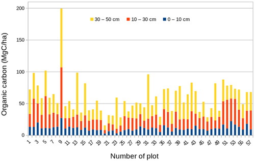
The total measured seagrass meadow TOC integrated across depths ranged from 15.5 to 199.3 Mg C ha⁻¹ (Figure 1S) with a mean value of 60.4 Mg C ha⁻¹ and a standard deviation (SD) of 27.5 Mg C ha⁻¹. Approximately 80% of the field data ranged between 15.5 and 70 Mg C ha⁻¹ and up to 99% of the field data varied from 15.5 to 100 Mg C ha⁻¹.

3.1. Seagrass total organic carbon estimation from remotely sensed data

The four selected ML models were first evaluated for each of the three scenarios that did not include feature optimization (Table 3). In all these three scenarios, the CB outperformed the RF, the XGB, and the RoF models with a highest value R² of 0.46. Surprisingly, for most models, there was little difference in performance for each of the scenarios 1 and 2, where only S-1 or S-2 bands were involved. A fusion of S-1 and S-2 sensors (scenario 3) improved the model skill with a slight increment of R² in cases of the XGB and the RoF model while the CB retrieved the TOC at a higher confidence (R² = 0.46, RMSE = 16.22 Mg C ha⁻¹, Table 3).

Table 3. Model performance of TOC estimation in scenario 1, scenario 2, scenario 3.

	Scenario 1					Scenario 2					Scenario 3
	R^2	RMSE	RMSE%	AIC	BIC	R^2	RMSE	RMSE%	AIC	BIC	R^2	RMSE	RMSE%	AIC	BIC
RF	0.24	19.33	63.06	194.24	227.17	0.24	19.30	57.71	180.17	205.15	0.20	19.89	64.27	239.56	297.47
XGB	0.32	18.32	52.65	191.79	224.71	0.31	18.48	55.88	178.17	203.15	0.33	18.11	49.69	235.25	293.16
CB	0.37	17.63	48.25	190.01	222.94	0.34	18.03	48.25	177.02	202.00	0.46	16.22	46.69	230.17	288.08
RoF	0.15	20.46	66.51	196.86	229.79	0.20	19.72	63.10	181.77	206.15	0.17	20.16	66.79	240.17	298.08

R² is used to compare model performance among scenarios while other metrics are opted for the evaluation of ML model in each of scenario due to a random splitting of the samples.

3.2. Improving of seagrass TOC estimation using feature selection method

To retrieve the TOC with accuracy, feature selection is often required to define a subset of the most significant input bands. Scenario 4 applied a Spearman correlation analysis to select these, while scenario 5 experimented an advanced metaheuristic GWO to select the most informative bands. All ML models for scenario 4 showed an improvement in TOC retrieval over scenarios 1–3 (Table 4 and Figure 4) with the RF, the XGB, and the RoF were converging on R² from 0.42 to 0.45 while the CB continued to yield a best performance with highest R² (0.53) and lowest RMSE (13.09 Mg C ha⁻¹). As the most accurate candidate, the CB was used as the base model in the GWO for feature selection, which resulted in a further improvement of the TOC retrieval accuracy (Table 4 and Figure 4).

Figure 4. Scatter plot of seagrass TOC estimation derived from ML models in scenario 4: (a–d) and scenario 5 (e): (a) RF, (b) XGB, (c) CB, (d) RoF, (e) CB-GWO.

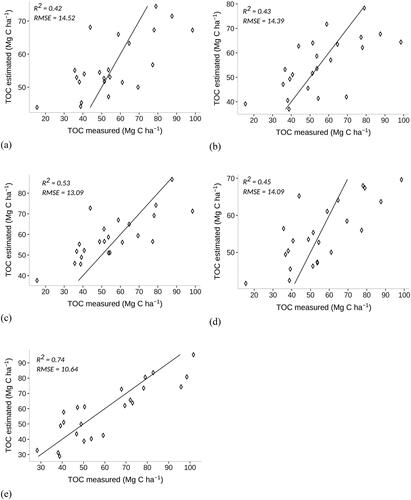
Table 4. Model performance of TOC estimation in scenario 4 and scenario 5.

	Scenario 4					Scenario 5
	R^2	RMSE	RMSE%	AIC	BIC	R^2	RMSE	RMSE%	AIC	BIC
RF	0.42	14.52	45.67	163.07	185.78
XGB	0.43	14.39	39.13	162.66	185.37
CB	0.53	13.09	38.49	158.31	181.02	0.74	10.64	19.58	152.78	177.76
RoF	0.45	14.09	42.44	161.70	184.41

R² is used to compare model performance among scenarios while other metrics are opted for the evaluation of ML model in each of scenario due to a random splitting of the samples.

As the best candidate for TOC estimation in designed scenarios, we visualized the CB performance in scenarios 3, 4, and 5 using the Taylor plot (Figure 2S). In the domains of the SD, correlation and RMSD, the CB model in scenario 5 presented a highest confidence for seagrass TOC estimation in the study site (the highest correlation coefficient and the lowest RMSD of the CBR_E3 observed in the Taylor plot, Figure 2S).

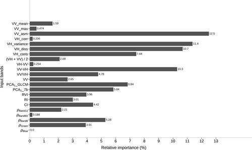
Of the 22 variables derived as informative from the GWO algorithm (Figure 5), S-2 contributed 8 bands (accounting for roughly 23%). The green, the near-infrared (NIR, band 8), and the short wavelength infrared (SWIR, band 12) contributed 11.4% while the transformed bands of the CI, the RI, the RVI supported a same ratio of 11.39% to the estimation of seagrass TOC. The S-1 sensor provided 14 meaningful bands (approximately 77% variation). The single band VV constituted 2.65% while 61.05% were imparted for the derived GLCM (44.30%), PCA (12.68%), and band ratio (17.42%). The CB indicated the S-2 NIR (band 8) and CI and the S-1 VV-VH, VH_diss, VH_variance and VV_asm as the most impact input variables on the accurate mapping of the seagrass TOC in Tauranga Harbour (Figure 5).

Figure 5. Variable contribution derived from the CB-GWO model for seagrass TOC estimation.

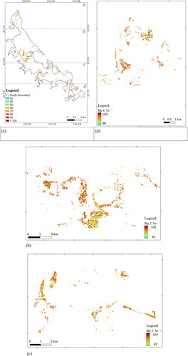
Using the CB-GWO model, the spatial variation of seagrass TOC in Tauranga Harbour (Figure 6) ranges from 30 to 104 Mg C ha⁻¹, with areas with TOC from 35 to 60 Mg C ha⁻¹ most frequent in the far north and the middle basin of the harbour (Figure 6(a,b)), while the middle and the southern basin mostly stored TOC > 60 Mg C ha⁻¹ (Figure 6(c,d)).

Figure 6. Seagrass TOC derived from the CB-GWO model and (a) the northern, (b) the upper middle, (c) the lower middle, (d) the southern parts in Tauranga Harbour.

4. Discussion

To successfully estimate the seagrass TOC from satellite sensing, we integrated a wide range of different approaches, multi-sensor satellite images, ML models, and advanced feature selection using the metaheuristic optimization. The results are promising with clear evidence that using both S-1, S-2 sensors modern ML models and methods of feature selection all improved overall prediction skill. The feature selection using the GWO algorithm improved the confidence of TOC estimation (R² = 0.74) to a magnitude of higher 60% and 39.6% compared to the accuracy in scenario 3 (R² = 0.46) without feature selection and scenario 4 (R² = 0.53) with the traditional Spearman feature selection.

Of the two bagging and boosting ML models, the boosting group, XGB and CB models, performs much better with a higher confidence (Table 3 and Table 4), with the CB model consistently the best in scenarios 1, 2, 3, and 4. The RoF model produced a relatively higher in R² score than the XGB, however was at higher RMSE% and therefore was less confident than the XGB model (Table 4, scenario 4). The performance of the CB model was found to be consistent with reports for mangrove and other ecosystems (Pham, Yokoya, et al. 2020; Ha et al. 2021a; Luo et al. 2021; Pham et al. 2021; Tran et al. 2021) in retrieving the biophysical parameters and carbon stock. The outperformance of the CB model for seagrass TOC estimation might be in part attributed to its novel ordered boosting mechanism, which mitigates overfitting, and its oblivious decision tree structure, which allows it to regularize the tree parameters to optimize different solutions, and hence reduces modelling uncertainty. In addition, the CB is recognized as working well with heterogeneous data types (i.e. mixture of different types of input data), and therefore may be expected to learn effectively from a fusion of both S-1 and S-2 data and derived variables.

Our study supports the use of feature selection and highlights the difference in the contribution of input variables to the final CB model. The Spearman analysis introduced a new subset of input variables, however it was evidences that correlation based selection was not sufficient to find the most contributed variables to the retrieval of TOC in this study. In converse, the metaheuristic GWO effect a good optimization in the search space, which results in the best combination of 22 input variables for the seagrass TOC retrieval in Tauranga Harbour. Metaheuristic optimization and the GWO algorithm, in particular are increasingly well-known methods for optimization of a wide ranges of problems (Abdel-Basset et al. 2018; Wong and Ming 2019; Agrawal et al. 2021). The potential application of this group method in the ecology and environmental science, however has not been discovered spaciously for a specific problem of accurate TOC estimation in seagrass ecosystems. The GWO mathematically simulates the hunting behaviour of the grey wolf herds, a well-known hunting strategy in the nature with the capability of relocating the solutions (i.e. updating positions of alpha, beta and delta wolfs to the solutions), and therefore is very powerful to discover the combination of input variables to archive the best solution under a given metric (i.e. the mean squared error in this study). In a n-dimensional search space, the GWO is designed to be self-adjustment to a balance of the exploitation (A parameter) and exploration (C parameter), and hence results in a fast convergence with less memory usage – the model structure using only one vector of position and three best saved solutions and computation time (Faris et al. 2018). For the seagrass TOC, we designed the objective function using the CB model with a medium size of both the iteration (200) and population (200), which appears to suit the estimation of the TOC in the complex coastal ecosystem. Figures indicated that TOC was sequestered to a lesser degree in the northern part (larger area with light green colour, Figure 6(a)) while more TOC was sequestered in the middle and southern parts of the harbour (Figure 6(b–d)). The variation of the TOC fit well with the dense and stable seagrass meadows (Ha et al. 2020), which supports better trapping and storage of carbon in the soil layers. The map indicated a spatial gradient of the TOC in different sub-spaces of the harbour, which can be assumed to reflect the different impacts of healthy seagrass, other biophysical parameters and topography of the catchment on carbon sequestration mechanisms (Samper-Villarreal et al. 2016; Alemu I et al. 2022). Furthermore targetted data collection and analysis may be required to evaluate, with confidence, specific impacts of the agriculture, urbanization and port business on the seagrass carbon sequestration in Tauranga Harbour.

Previous studies targeting carbon stock estimation using remote sensing across a variety of ecosystem types (though not seagrass ecosystem) reported a variation of accuracy broadly similar to that shown here (R² ranges 0.6–0.87) (Wicaksono et al. 2016; Sanderman et al. 2018; Pham et al. 2021; Sun et al. 2021; Nguyen et al. 2022). Seagrass meadows can be expected to be difficult for such estimates, as the above-ground biomass collapses at low tide, when sensing is possible, and a high proportion of carbon is below ground. Unlike above-ground parameters (above-ground biomass, spatial distribution, canopy height, for instances), the below-ground carbon stock requires either an indirect approach using different soil/vegetation indexes, input band transformation or longer wavelength SAR sensors (ALOS-2 PALSAR-2 with L band, for instance), in which the band is capable of penetrating deeper into the layers below the soil surface. Since the S-1 C-band penetrates only to a few centimetres below the surface, our estimates are likely indirect, and this is consistent with inputs from a variety of image transformation (band ratio, GLCM, PCA). The use of SAR only, multi-spectral only, or fusion of both, resulted in low retrieval accuracy in scenarios 1–3. High accuracy was only obtained in scenario 5 with GWO and the CB feature importance function determined a larger contribution proportion of S-1 (nearly 77%) than S-2 (approximately 23%) sensor to the final model. This indicates the advantage of satellite data fusion to achieve high confidence mapping of seagrass meadow TOC. The variation in carbon stock therefore likely correlates to both the colour, texture of the soil surface (Nguyen et al. 2022) and the above-ground vegetation structure (Xue and Su 2017; Morcillo-Pallarés et al. 2019). As expected, the green, red and NIR spectra (band 8 and CI indexes, S-2 sensor), which strongly reflect the variation in the soil/vegetation, significantly contributed to the success retrieval of TOC. The contribution from S-1 (transformed) bands were found similar for carbon stock in other ecosystems (Byrd et al. 2018; Nguyen et al. 2022) or seagrass above-ground biomass estimation (Ha et al. 2021a) and may prefect a correlation between the surface features and the presence of dense, species diverse and carbon-rich seagrass meadows. Our case study determined the VV band and the transformation of VV-VH and GLCM (VH_diss, VH_variance and VV_asm) to have the most useful information on the vegetation structure or soil texture to the accurate estimation of seagrass TOC in Tauranga Harbour.

The methods developed and results obtained in this study provide novel insights into TOC retrieval using a suite of the state-of-the-art remote sensing, modelling and feature selection tools. The proposed framework is solid and reliable, using the advanced models and high quality remotely sensed data, it is applicable and very low cost since we use only open access remote sensing data and the open source codes for image processing, modelling and optimization. The processing codes adapted in this research are all available in the GitHub (https://github.com/), SourceForge (https://sourceforge.net/) or well-developed and independent open source project (Sentinel Toolbox (https://sentinel.esa.int/web/sentinel/toolboxes), QGIS (https://www.qgis.org/en/site/)), which guarantees for a wide exchange in method and further extending to other blue carbon ecosystems and improves the certainty in global blue carbon estimation in the future. High temporal resolution (5–12 days) of both S-1 and S-2 sensors supports users to locate more acquired images to find the best scenes fitting their study site. In addition, the band transformation will provide more options for model fitting, rather than the two original bands of S-1 and 12 original bands of S-2 sensors, in deriving critical information for the retrieval model.

Our research, however was narrowed to the C-band of S-1 sensor, and constrained by the need for low tide to sense the intertidal zones. In addition, we acknowledge that the TOC mapping was only produced for the vegetated areas (i.e. seagrass meadows) in Tauranga Harbour. The proposed CB-GWO model is able to explain 74% of spatial TOC distribution with a degree of prediction variation (Figure 3S) in the study site. The model performance indicates challenges and leaves a degree of uncertainty in the quantification of the seagrass TOC. Beside the complexity in seagrass meadow structure in the intertidal zone which might increase the noise in satellite signal retrieval, the must-use indirect approach for soil properties estimate in dense covered vegetation also contributes to the uncertainty of retrieval models for seagrass TOC quantification in the coastal zones. Future field surveys will need to cover a wider range of sediment samples, including both vegetated and unvegetated areas in the intertidal zones, to provide more intensive data for our proposed methods. New research is underway with experiments for a variety of seagrass species in different bio-ecological regions, using the same approach with novel ML models or better feature selection algorithms.

5. Conclusion

Seagrass TOC is an important biophysical parameter with unsolved challenges for accurate estimation worldwide. We have developed a novel and effective approach using the fusion of multi-spectral and SAR satellite images, integrated with CatBoost machine learning technique and the GWO algorithm (CB-GWO) to derive and map TOC distribution across seagrass meadows in a large New Zealand estuary. Five scenarios of performance were designed, which indicated that neither S-1, S2 nor a fusion of all S-1, S-2 bands derived with high precision the variation of TOC, and that feature selection was required to extract the most contributed input variables. In addition to the well-known RF and the XGB models, this study highlights the better performance of the CatBoost model combined with GWO, the CB-GWO (R² = 0.74, RMSE = 10.64 Mg C ha⁻¹, RMSE% = 19.58%) and the potential use of the RoF model for further improvement of TOC estimation. Feature selection using metaheuristic optimization with the GWO algorithm improved the accuracy up to 60% in comparison to the same models run without feature selection.

Our proposed method is robust and applicable, easy to implement with open-source codes for machine learning algorithms, image processing and metaheuristic optimization. The workflows presented in this study are not limited to the ecosystem of seagrass, rather the methods of image analysis and modelling are rationale to apply to various biophysical parameters in different blue carbon ecosystems (i.e. mangrove forest, salt-marsh). In addition, we suggest the using of the GWO for an accurate selection of input variables in further multi-modal data analysis of inventory and conservation of blue carbon ecosystems. This approach, however also comes with an unavoidable drawback of the SAR image application. Due to the attenuation of the SAR signal in the water environment, we suggest the use of the proposed methods for the intertidal regions where the habitats are exposed at the low tide and the SAR image could be used effectively to derive more accurate the variation of TOC.

Future field survey campaigns will validate and expand our proposed method for seagrass TOC retrieval in different climate regions worldwide. In addition, a comparison of various metaheuristic algorithms for feature selection is proposed discover and better understand the contribution of multi-spectral and SAR image bands for the estimation of seagrass TOC.

Author contributions

All authors have read and agree to the published version of the manuscript. Conceptualization, N.T.H and I.H; methodology, N.T.H.; software, N.T.H. and T.D.P.; validation, N.T.H. and T.D.P; resources, N.T.H, T.H.P, I.H; writing-original draft preparation, N.T.H.; writing-review and editing, N.T.H., T.D.P., T.H.P, D.A.T and I.H. All authors have read and agreed to the published version of the manuscript.

Acknowledgements

We sincerely thank the staff in the Marine Field Station, Tauranga, New Zealand who assisted us during the field survey conducted in Tauranga Harbour, New Zealand.

Disclosure statement

No potential conflict of interest was reported by the author(s).

Data availability statement

The data that support the findings of this study are available from the corresponding author, Nam-Thang Ha, upon reasonable request.

Additional information

Funding

The authors acknowledge the partial support of University of Agriculture and Forestry, Hue University under the Strategic Research Group Program, Grant No. NCM.ĐHNL.2021.03: GIS, remote sensing, and precision farming.

References

- Abdel-Basset M, Abdel-Fatah L, Sangaiah AK. 2018. Chapter 10 – Metaheuristic algorithms: a comprehensive review. In: Sangaiah AK, Sheng M, Zhang Z, editors. Computational intelligence for multimedia big data on the cloud with engineering applications. Cambridge, Massachusetts, US: Academic Press; p. 185–231.
- Agrawal P, Abutarboush HF, Ganesh T, Mohamed AW. 2021. Metaheuristic algorithms on feature selection: a survey of one decade of research (2009–2019). IEEE Access. 9:26766–26791.
- Ahmad H. 2019. Machine learning applications in oceanography. Aquat Res.:161–169.
- Alemu IJB, Yaakub SM, Yando ES, San Lau RY, Chang Lim C, Puah JY, Friess DA. 2022. Geomorphic gradients in shallow seagrass carbon stocks. Estuarine Coastal Shelf Sci. 265:107681.
- Bedulli C, Lavery PS, Harvey M, Duarte CM, Serrano O. 2020. Contribution of seagrass blue carbon toward carbon neutral policies in a touristic and environmentally-friendly island. Front Mar Sci. 7:1.
- Breiman L. 2001. Random Forest. Machine Learning. 45(1):5–32.
- Bulmer RH, Townsend M, Drylie T, Lohrer AM. 2018. Elevated turbidity and the nutrient removal capacity of seagrass. Front Mar Sci. 5:462.
- Byrd KB, Ballanti L, Thomas N, Nguyen D, Holmquist JR, Simard M, Windham-Myers L. 2018. A remote sensing-based model of tidal marsh aboveground carbon stocks for the conterminous United States. ISPRS J Photogramm Remote Sens. 139:255–271.
- Chen T, Guestrin C. 2016. XGBoost: a scalable tree boosting system. In: Proceedings of the 22nd ACM SIGKDD International Conference on Knowledge Discovery and Data Mining – KDD ’16 [Internet]. San Francisco (CA): ACM Press; [accessed 2019 Dec 27]; p. 785–794. https://doi.org/10.1145/2939672.2939785.
- Cussioli MC, Bryan KR, Pilditch CA, de Lange WP, Bischof K. 2019. Light penetration in a temperate meso-tidal lagoon: implications for seagrass growth and dredging in Tauranga Harbour, New Zealand. Ocean Coast Manag. 174:25–37.
- Dorogush AV, Ershov V, Gulin A. 2018. CatBoost: gradient boosting with categorical features support [Internet]; [accessed 2022 Dec 25]. https://doi.org/10.48550/arXiv.1810.11363.
- Duarte CM, Kennedy H, Marbà N, Hendriks I. 2013. Assessing the capacity of seagrass meadows for carbon burial: current limitations and future strategies. Ocean Coast Manag. 83:32–38.
- Ellis J, Cawthron T. 2013. Ecological survey of Tauranga Harbour [accessed 2022 May 30]. https://www.researchgate.net/publication/271197663_Ecological_Survey_of_Tauranga_Harbour.
- Environment Bay of Plenty. 2010. Soils of the Bay of Plenty Volume 1. [accessed 2021 Dec 20]. https://www.boprc.govt.nz/media/32401/EnvReport-201011-SoilsBayofPlentyV1WesternBay.pdf.
- ESA. 2020. Toolboxes – STEP. [accessed 2022 Jan 8]. https://step.esa.int/main/toolboxes/.
- ESA-S1. 2020. Sentinel-1 SAR. [accessed 2020 Aug 24]. https://sentinel.esa.int/web/sentinel/user-guides/sentinel-1-sar.
- Ewers Lewis CJ, Young MA, Ierodiaconou D, Baldock JA, Hawke B, Sanderman J, Carnell PE, Macreadie PI. 2020. Drivers and modelling of blue carbon stock variability in sediments of southeastern Australia. Biogeosciences. 17(7):2041–2059.
- Ezenkwu CP, Akpan UI, Stephen BU-A. 2021. A class-specific metaheuristic technique for explainable relevant feature selection. Mach Learn Appl. 6:100142.
- Faris H, Aljarah I, Al-Betar MA, Mirjalili S. 2018. Grey wolf optimizer: a review of recent variants and applications. Neural Comput Appl. 30(2):413–435.
- Filipponi F. 2019. Sentinel-1 GRD preprocessing workflow. Multidiscip Digit Publish Inst Proc. 18(1):11.
- Fourqurean JW, Duarte CM, Kennedy H, Marbà N, Holmer M, Mateo MA, Apostolaki ET, Kendrick GA, Krause-Jensen D, McGlathery KJ, et al. 2012. Seagrass ecosystems as a globally significant carbon stock. Nat Geosci. 5(7):505–509.
- Githaiga MN, Kairo JG, Gilpin L, Huxham M. 2017. Carbon storage in the seagrass meadows of Gazi Bay, Kenya. PLoS One. 12(5):e0177001.
- Grubb M, Okereke C, Arima J, Bosetti V, Chen Y, Edmonds J, Gupta S, Köberle A, Kverndokk S, Malik A, et al. 2022. Introduction and framing. In IPCC, 2022: Climate Change 2022: Mitigation of Climate Change. Contribution of Working Group III to the Sixth Assessment Report of the Intergovernmental Panel on Climate Change. Cambridge (UK): Cambridge University Press.
- Ha N-T, Manley-Harris M, Pham TD, Hawes I. 2020. A comparative assessment of ensemble-based machine learning and maximum likelihood methods for mapping seagrass using Sentinel-2 imagery in Tauranga Harbor, New Zealand. Remote Sens. 12(3):355.
- Ha N-T, Manley-Harris M, Pham TD, Hawes I. 2021a. The use of radar and optical satellite imagery combined with advanced machine learning and metaheuristic optimization techniques to detect and quantify above ground biomass of intertidal seagrass in a New Zealand estuary. Int J Remote Sens. 42(12):4712–4738.
- Ha N-T, Manley-Harris M, Pham T-D, Hawes I. 2021b. Detecting multi-decadal changes in seagrass cover in Tauranga Harbour, New Zealand, using Landsat imagery and boosting ensemble classification techniques. ISPRS Int J Geo-Inf. 10(6):371.
- Hilmi N, Chami R, Sutherland MD, Hall-Spencer JM, Lebleu L, Benitez MB, Levin LA. 2021. The role of blue carbon in climate change mitigation and carbon stock conservation. Front Clim. 3:710546.
- Howard J, Hoyt S, Isensee K, Pidgeon E, Telszewski M. 2014. Coastal Blue Carbon: methods for assessing carbon stocks and emissions factors in mangroves, tidal salt marshes, and seagrass meadows. Telszewski M, editor. Arlington (VA): Intergovernmental Oceanographic Commission of UNESCO, International Union for Conservation of Nature.
- IPCC. 2019. Special report on the ocean and cryosphere in a changing climate. Cambridge (UK): Cambridge University Press.
- James RK, Christianen MJA, Katwijk MM, Smit JC, Bakker ES, Herman PMJ, Bouma TJ. 2020. Seagrass coastal protection services reduced by invasive species expansion and megaherbivore grazing. J Ecol. 108(5):2025–2037.
- Jankowska E, Michel LN, Lepoint G, Włodarska-Kowalczuk M. 2019. Stabilizing effects of seagrass meadows on coastal water benthic food webs. J Exp Mar Biol Ecol. 510:54–63.
- Jiang Z, Huang D, Fang Y, Cui L, Zhao C, Liu S, Wu Y, Chen Q, Ranvilage CIPM, He J, et al. 2020. Home for marine species: seagrass leaves as vital spawning grounds and food source. Front Mar Sci. 7:194.
- Lary DJ, Alavi AH, Gandomi AH, Walker AL. 2016. Machine learning in geosciences and remote sensing. Geosci Front. 7(1):3–10.
- Le NN, Pham TD, Yokoya N, Ha NT, Nguyen TTT, Tran TDT, Pham TD. 2021. Learning from multimodal and multisensor earth observation dataset for improving estimates of mangrove soil organic carbon in Vietnam. Int J Remote Sens. 42(18):6866–6890.
- Lincoln S, Vannoni M, Benson L, Engelhard GH, Tracey D, Shaw C, Molisa V. 2021. Assessing intertidal seagrass beds relative to water quality in Vanuatu, South Pacific. Mar Pollut Bull. 163:111936.
- Luo M, Wang Y, Xie Y, Zhou L, Qiao J, Qiu S, Sun Y. 2021. Combination of feature selection and CatBoost for prediction: the first application to the estimation of aboveground biomass. Forests. 12(2):216.
- Macreadie PI, Anton A, Raven JA, Beaumont N, Connolly RM, Friess DA, Kelleway JJ, Kennedy H, Kuwae T, Lavery PS, et al. 2019. The future of Blue Carbon science. Nat Commun. 10(1):3998.
- Maddio S, Pelosi G, Righini M, Selleri S. 2019. A comparison between grey wolf and invasive weed optimizations applied to microstrip filters. In 2019 IEEE International Symposium on Antennas and Propagation and USNC-URSI Radio Science Meeting. p. 1033–1034.
- Mahdianpari M, Salehi B, Mohammadimanesh F, Homayouni S, Gill E. 2018. The first wetland inventory map of Newfoundland at a spatial resolution of 10 m using Sentinel-1 and Sentinel-2 data on the Google Earth Engine cloud computing platform. Remote Sens. 11(1):43.
- Mari L, Melià P, Gatto M, Casagrandi R. 2021. Identification of ecological hotspots for the seagrass Posidonia oceanica via metapopulation modeling. Front Mar Sci. 8:456.
- McHenry J, Rassweiler A, Hernan G, Uejio CK, Pau S, Dubel AK, Lester SE. 2021. Modelling the biodiversity enhancement value of seagrass beds. Divers Distrib. 27(11):2036–2049.
- Mirjalili S, Mirjalili SM, Lewis A. 2014. Grey wolf optimizer. Adv Eng Softw. 69:46–61.
- Morcillo-Pallarés P, Rivera-Caicedo JP, Belda S, De Grave C, Burriel H, Moreno J, Verrelst J. 2019. Quantifying the robustness of vegetation indices through global sensitivity analysis of homogeneous and forest leaf-canopy radiative transfer models. Remote Sens. 11(20):2418.
- Muttil N, Chau K-W. 2007. Machine-learning paradigms for selecting ecologically significant input variables. Eng Appl Artif Intell. 20(6):735–744.
- Naud C, Courrech C, De Gauiac H. 2021. Sentinel-2 products specification document. [accessed 2020 Jul 23]. https://sentinel.esa.int/documents/247904/685211/Sentinel-2-Products-Specification-Document.
- Navarro JA, Algeet N, Fernández-Landa A, Esteban J, Rodríguez-Noriega P, Guillén-Climent ML. 2019. Integration of UAV, Sentinel-1, and Sentinel-2 data for mangrove plantation aboveground biomass monitoring in Senegal. Remote Sens. 11(1):77.
- Nguyen TT, Pham TD, Nguyen CT, Delfos J, Archibald R, Dang KB, Hoang NB, Guo W, Ngo HH. 2022. A novel intelligence approach based active and ensemble learning for agricultural soil organic carbon prediction using multispectral and SAR data fusion. Sci Total Environ. 804:150187.
- Nielsen DS. 2022. Doubt. [accessed 2022 Sep 9]. https://github.com/saattrupdan/doubt.
- Nordlund LM, Koch EW, Barbier EB, Creed JC. 2016. Seagrass ecosystem services and their variability across genera and geographical regions. PLoS One. 11(10):e0163091.
- Orth RJ, Lefcheck JS, McGlathery KS, Aoki L, Luckenbach MW, Moore KA, Oreska MPJ, Snyder R, Wilcox DJ, Lusk B. 2020. Restoration of seagrass habitat leads to rapid recovery of coastal ecosystem services. Sci Adv. 6(41):eabc6434.
- Park SG. 1999. Changes in abundance of seagrass (Zostera spp.) in Tauranga Harbour from 1959–96. Whakatane, New Zealand [accessed 2019 Oct 11]. https://cdn.boprc.govt.nz/media/362713/changes-in-abundance-of-seagrass-zostera-spp-in-tauranga-harbour-from-1959-96.pdf.
- Pedregosa F, Varoquaux G, Gramfort A, Michel V, Thirion B, Grisel O, Blondel M, Prettenhofer P, Weiss R, Dubourg V, et al. 2011. Scikit-Learn: machine learning in Python. J Mach Learn Res. 12:2825–2830.
- Pham TD, Le NN, Ha NT, Nguyen LV, Xia J, Yokoya N, To TT, Trinh HX, Kieu LQ, Takeuchi W. 2020. Estimating mangrove above-ground biomass using extreme gradient boosting decision trees algorithm with fused Sentinel-2 and ALOS-2 PALSAR-2 data in can Gio Biosphere Reserve, Vietnam. Remote Sens. 12(5):777.
- Pham TD, Xia J, Ha NT, Bui DT, Le NN, Tekeuchi W. 2019. A review of remote sensing approaches for monitoring blue carbon ecosystems: mangroves, seagrasses and salt marshes during 2010–2018. Sensors. 19(8):1933.
- Pham TD, Yokoya N, Nguyen TTT, Le NN, Ha NT, Xia J, Takeuchi W, Pham TD. 2021. Improvement of mangrove soil carbon stocks estimation in North Vietnam using Sentinel-2 data and machine learning approach. GISci Remote Sens. 58(1):68–87.
- Pham TD, Yokoya N, Xia J, Ha NT, Le NN, Nguyen TTT, Dao TH, Vu TTP, Pham TD, Takeuchi W. 2020. Comparison of machine learning methods for estimating mangrove above-ground biomass using multiple source remote sensing data in the Red River Delta Biosphere Reserve, Vietnam. Remote Sensing. 12(8):1334.
- Potouroglou M, Bull JC, Krauss KW, Kennedy HA, Fusi M, Daffonchio D, Mangora MM, Githaiga MN, Diele K, Huxham M. 2017. Measuring the role of seagrasses in regulating sediment surface elevation. Sci Rep. 7(1):1–11.
- Prokhorenkova L, Gusev G, Vorobev A, Dorogush AV, Gulin A. 2019. CatBoost: unbiased boosting with categorical features. arXiv:170609516 [cs] [Internet]; [accessed 2019 Dec 26]. http://arxiv.org/abs/1706.09516
- Reeve G, Stephens SA, Wadhwa A. 2018. Tauranga Harbour inundation modelling. Tauranga, New Zealand: NIWA.
- Rodriguez JJ, Kuncheva LI, Alonso CJ. 2006. Rotation forest: a new classifier ensemble method. IEEE Trans Pattern Anal Mach Intell. 28(10):1619–1630.
- Saiz G, Albrecht A. 2016. Methods for smallholder quantification of soil carbon stocks and stock changes. In Rosenstock TS, Rufino MC, Butterbach-Bahl K, Wollenberg L, Richards M, editors. Methods for measuring greenhouse gas balances and evaluating mitigation options in smallholder agriculture. Cham: Springer International Publishing; p. 135–162.
- Salinas C, Duarte CM, Lavery PS, Masque P, Arias‐Ortiz A, Leon JX, Callaghan D, Kendrick GA, Serrano O. 2020. Seagrass losses since mid-20th century fuelled CO2 emissions from soil carbon stocks. Glob Chang Biol. 26(9):4772–4784.
- Samper-Villarreal J, Lovelock CE, Saunders MI, Roelfsema C, Mumby PJ. 2016. Organic carbon in seagrass sediments is influenced by seagrass canopy complexity, turbidity, wave height, and water depth. Limnol Oceanogr. 61(3):938–952.
- Sanderman J, Hengl T, Fiske G, Solvik K, Adame MF, Benson L, Bukoski JJ, Carnell P, Cifuentes-Jara M, Donato D, et al. 2018. A global map of mangrove forest soil carbon at 30 m spatial resolution. Environ Res Lett. 13(5):055002.
- Sani DA, Hashim M, Hossain MS. 2019. Recent advancement on estimation of blue carbon biomass using satellite-based approach. Int J Remote Sens. 40(20):7679–7715.
- Singh J. 2021. Zoofs [accessed 2022 Jan 11].
- Smith P, Soussana J-F, Angers D, Schipper L, Chenu C, Rasse DP, Batjes NH, van Egmond F, McNeill S, Kuhnert M, et al. 2020. How to measure, report and verify soil carbon change to realize the potential of soil carbon sequestration for atmospheric greenhouse gas removal. Glob Chang Biol. 26(1):219–241.
- Sricharan K, Srivistava A. 2012. Bootstrap prediction intervals in non-parametric regression with applications to anomaly detection. [accessed 2022 Sep 1]. https://ntrs.nasa.gov/api/citations/20130014367/downloads/20130014367.pdf.
- Stankovic M, Ambo-Rappe R, Carly F, Dangan-Galon F, Fortes MD, Hossain MS, Kiswara W, Van Luong C, Minh-Thu P, Mishra AK, et al. 2021. Quantification of blue carbon in seagrass ecosystems of Southeast Asia and their potential for climate change mitigation. Sci Total Environ. 783:146858.
- Sun S, Wang Y, Song Z, Chen C, Zhang Y, Chen X, Chen W, Yuan W, Wu X, Ran X, et al. 2021. Modelling aboveground biomass carbon stock of the Bohai Rim coastal wetlands by integrating remote sensing, terrain, and climate data. Remote Sens. 13(21):4321.
- Susi R, Udhi EH, Kathryn M, Bayu P, Hanif BP, A’an JW, Mat V. 2019. Blue carbon in seagrass ecosystem: guideline for the assessment of carbon stock and sequestration in Southeast Asia. Yogyakarta, Indonesia: UGM Press.
- Tara JA, Mark M, Alison M, Malcolm C, Roberta D, Nelson W, Tracey D, Gordon D, Read G, Kettles H, et al. 2019. Review of New Zealand’s key biogenic habitats [accessed 2022 Sep 9]. https://www.mfe.govt.nz/sites/default/files/media/Marine/NZ-biogenic-habitat-review.pdf.
- Tay H, Bryan K, de Lange W, Pilditch C. 2013. The hydrodynamics of the southern basin of Tauranga Harbour. N Z J Mar Freshw Res. 47(2):249–274.
- Taylor KE. 2001. Summarizing multiple aspects of model performance in a single diagram. J Geophys Res. 106(D7):7183–7192.
- Thorhaug A, Poulos HM, López-Portillo J, Ku TCW, Berlyn GP. 2017. Seagrass blue carbon dynamics in the Gulf of Mexico: stocks, losses from anthropogenic disturbance, and gains through seagrass restoration. Sci Total Environ. 605–606:626–636.
- Tran DA, Tsujimura M, Ha NT, Nguyen VT, Binh DV, Dang TD, Doan Q-V, Bui DT, Anh Ngoc T, Phu LV, et al. 2021. Evaluating the predictive power of different machine learning algorithms for groundwater salinity prediction of multi-layer coastal aquifers in the Mekong Delta, Vietnam. Ecol Indic. 127:107790.
- Vanhellemont Q. 2016. ACOLITE for Sentinel-2: aquatic applications of MSI imagery. In Proceedings of the 2016 ESA Living Planet Symposium. Prague, Czech Republic: ESA Special Publication; p. 8.
- Vanhellemont Q. 2019. Adaptation of the dark spectrum fitting atmospheric correction for aquatic applications of the Landsat and Sentinel-2 archives. Remote Sens Environ. 225:175–192.
- Vrieze SI. 2012. Model selection and psychological theory: a discussion of the differences between the Akaike information criterion (AIC) and the Bayesian information criterion (BIC). Psychol Methods. 17(2):228–243.
- Wicaksono P, Danoedoro P, Nehren, U, Hartono. 2016. Mangrove biomass carbon stock mapping of the Karimunjawa Islands using multispectral remote sensing. Int J Remote Sens. 37(1):26–52.
- Wong W, Ming CI. 2019. A review on metaheuristic algorithms: recent trends, benchmarking and applications. In 2019 7th International Conference on Smart Computing Communications (ICSCC); p. 1–5.
- Xue J, Su B. 2017. Significant remote sensing vegetation indices: a review of developments and applications. J Sens. 2017:1–17.
- Yang R, Rossiter DG, Liu F, Lu Y, Yang F, Yang F, Zhao Y, Li D, Zhang G. 2015. Predictive mapping of topsoil organic carbon in an alpine environment aided by Landsat TM. PLoS One. 10(10):e0139042.
- Yang R-M, Guo W-W. 2019. Modelling of soil organic carbon and bulk density in invaded coastal wetlands using Sentinel-1 imagery. Int J Appl Earth Obs Geoinf. 82:101906.