Identification and delineation of groundwater-dependent ecosystems (GDEs) in the Khakea–Bray transboundary aquifer region using geospatial techniques

Abstract

Identifying and delineating groundwater-dependent ecosystems (GDEs) is critical in understanding their location, distribution and groundwater allocation. However, this information is inadequately understood due to limited available data for most areas where they occur. Thus, this study aims to address this gap using remotely sensed, analytical hierarchy process (AHP) and in situ data to identify and delineate GDEs in the Khakea–Bray transboundary aquifer region. The study tested various spatial-explicit GDE indices that integrates environmental factors that predict occurrence of GDEs. These include the normalized difference vegetation index as a proxy for vegetation productivity and modified normalized difference water index as proxy for moisture availability, land-use and landcover, topographical factors such as slope, topographic wetness index, flow accumulation and curvature. The GDEs were delineated using the weighted overlay tool in a Geographic Information System (GIS) environment. The thematic output layer was then spatially classified into two classes, namely, GDEs and non-GDEs. The results showed that only 1.34% of the area is characterised by GDEs covering 721,908 ha. Overall, identified GDEs were found mostly on a gentle slope on the large portion of shrubland and grassland. The derived GDEs map was then statistically compared with groundwater level (GWL) data from 22 boreholes that occur in the area. Our results indicated that: GDEs are concentrated at the northern, central and south-western part of the study area. The validation results showed significant overlapping of GDEs classes with both the groundwater level (GWL) and rainfall in the study area. The results show a possible delineation of GDEs in the study area using remote sensing and GIS techniques along with AHP and is transferable to other arid and semiarid environments. The results of this study contributes to identifying and delineating priority areas where appropriate water conservation programmes for sustainable groundwater development can be implemented.

Keywords:

• Analytical hierarchy process
• explanatory variables
• groundwater-dependent ecosystems
• Khakea–Bray transboundary aquifer
• Sentinel-2

1. Introduction

The sustainable management of groundwater-dependent ecosystems (GDEs) is critical given their ecological role and biodiversity conservation. GDEs can be divided mainly into terrestrial and aquatic systems. They include rivers (riparian habitats), lakes, forests and bushes, grasslands, wetlands, seeps and springs, as well as estuarine and coastal ecosystems (Kløve et al. 2011; Doody et al. 2017; Duran-Llacer et al. 2021; Liu et al. 2021). Specifically, they provide several ecological and socio-economic benefits, for example, ecological services such as carbon sequestration, water purification and mitigation amongst floods and droughts (Doody et al. 2019; Yang and Liu 2020; Dalu and Wasserman 2021). Furthermore, GDEs supports livelihoods through the provision of access to clean water, protection from natural disaster such as floods and droughts. In addition, they act as tourism attraction sites especially wetlands as they may have cultural significant and economic value (Kumar and Kanaujia 2014; Chaikumbung et al. 2016).

Despite their ecological and socio-economic benefits, climate variability and anthropogenic activities threaten GDEs’ ability to provide key ecological services. GDEs’ health and sustainability are threatened through excessive groundwater extraction (Eamus and Froend 2006; Kløve et al. 2011; Erostate et al. 2020; Williams et al. 2022). Groundwater is used in many ways in semiarid environments which include household, industrial and agricultural uses (Mango et al. 2017; Dube et al. 2020; Gronwall and Danert 2020; Verlicchi and Grillini 2020). Khakea–Bray transboundary aquifer region is amongst the areas that experience rapid increase in water abstraction for agriculture and domestic use. Consequently, the structure and functions of these ecosystems can be easily degraded owing to limits to groundwater availability and the absence of surface-water resources (Howard and Merrifield 2010; Orellana et al. 2012; Liu et al. 2021).

Although GDEs are distributed all over the world, they are not fully documented particularly in transboundary aquifers of water-limited regions (Liu et al. 2021). Limited research has been undertaken to delineate GDE in southern Africa. Studies of GDEs in transboundary aquifers focused on their impact of climate change (Majola et al. 2021), vegetation diversity (Mpakairi et al. 2022). However, spatial extent of GDEs in transboundary aquifers is underexplored and are poorly understood (Altchenko and Villholth 2013). This might be because GDE studies and management are limited to a few jurisdictions globally while they cross international borders (Rohde et al. 2017). Documenting their distribution and understanding their status is critical for their conservation as these ecosystems rely on groundwater on a temporary or permanent basis to sustain their structure, function and productivity (Howard and Merrifield 2010; Duran-Llacer et al. 2021; Rohde et al. 2021; Saito et al. 2021; Brim Box et al. 2022). The groundwater resources in these transboundary aquifers are challenging to monitor or manage for most partner countries (Mpakairi et al. 2022). Additionally, Mpakairi et al. (2022) found that vegetation in Khakea–Bray transboundary aquifer is diverse particularly around natural water pans and along rivers and roads. Thus, the GDEs in these areas provide several benefits such as water purification and nutrient cycling even though their spatial extent is unknown. There is a need to identify and delineate the location and spatial extent of GDEs, respectively, particularly in transboundary aquifer of semiarid environments to ensure sustainable GDEs management during current climate and anthropogenic change. This emphasises the necessity to delineate GDEs in Khakea–Bray transboundary aquifer region.

Accurate GDEs delineation forms the foundation for their definition and mapping, and is of great significance for GDEs conservation management and research (Rohde et al. 2017; Zheng et al. 2017). The use of GDEs identification methods depends largely on the extent of the area under study and its accessibility. For instance, the identification of GDEs at local scale can be based on stable isotope techniques to determine whether these systems use groundwater (Howard and Merrifield 2010; Miller et al. 2010; Orellana et al. 2012; Koit et al. 2021; Liu et al. 2021). However, this method is challenging in regional scale assessments (Eamus and Froend 2006; Eamus et al. 2015; Kuginis et al. 2016). Thus, studies are currently applying spatial explicit method such as remote sensing which provides robust, rapid and spatially extensive monitoring of GDEs (Eamus et al. 2015; Glanville et al. 2016; Tian et al. 2016; Ghosh and Das 2020; Kibler et al. 2021). Remote sensed data provide an opportunity to extract GDEs’ spatial extent since they occur in various sizes, over space and time and their aspects such as water and vegetation variability over time.

Studies (e.g. Münch and Conrad 2007; Gou et al. 2015; Chiloane et al. 2020; Gxokwe et al. 2020; Zwedzi 2020; Duran-Llacer et al. 2021; Liu et al. 2021; Martínez-Santos et al. 2021;  Thamaga et al. 2021) have indicated the capability of multispectral sensors such as Landsat-8 OLI with the advanced sensing design and Sentinel-2 with 10, 20 and 60 m spatial resolutions, with 5-day revisit period which allows the detection of GDEs spatial coverage in remote areas. These studies utilized image classification methods, multispectral or hyperspectral derived indices together with machine learning algorithms (Rapinel et al. 2019). For example, Chiloane et al. (2020) indicated the successful groundwater-dependent terrestrial vegetation identification using Sentinel derived normalized difference vegetation index (NDVI) with accuracy of 95% in the Greater Floristic Region of the Western Cape province, South Africa. In a different study, Liu et al. (2021) utilised to remote sensed data to map GDEs in central Asia. Furthermore, Dresel et al. (2010) developed an integrated method using the derived Moderate Resolution Imaging Spectroradiometer (MODIS)-Enhanced Vegetation Index (EVI) and derived Landsat-NDVI coupled with image classification, to identify GDEs at Victoria in Australia, whereas Gou et al. (2015) proposed a GDE index and combined three remote sensing measures to identify potential GDEs in Texas, USA.

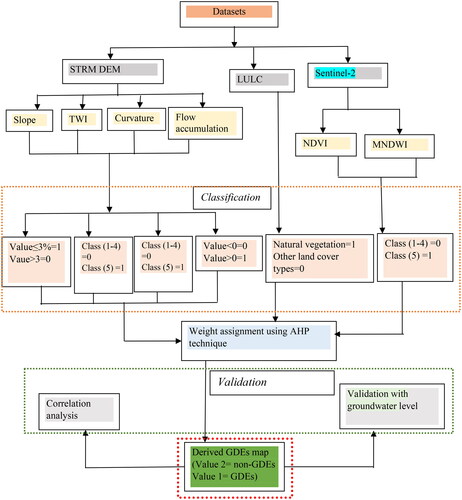
Thus, this study aims to identify and delineate GDEs spatial extent using different method of Sentinel-2 MSI derived spectral indices together with analytical hierarchy process (AHP) in Geographic Information System (GIS) environment in Khakea–Bray transboundary aquifer region. This method integrates a multicriteria process based on expert opinion, GIS techniques, remote sensing and field work. Additionally, it includes geospatial information including land-use and landcover (LULC), topographical parameters such as topographic wetness index (TWI), slope, curvature and flow accumulation, multispectral indices such as NDVI and modified normalized difference water index (MNDWI). Hence, this method allows the GDEs to be delineated and is transferable to other arid and semiarid environments.

2. Materials and methods

2.1. Study area

The study was conducted in Khakea–Bray transboundary aquifer region that is situated on the border of South Africa and Botswana (Figure 1). Khakea–Bray transboundary aquifer region is situated on a dolomitic outcrop of the Campbell–Rand dolomites and overlain by Kalahari sands stretching from South Africa to Botswana (Carlsson et al. 2009; Haasbroek 2018). Intergranular (porous) covers a small portion in part of South African on the Kalahari Beds. The intergranular aquifer is characterised by the borehole yield of medium of 1.8–7.2 m³/h and highest of >7.2 m³/h. The dolomite as well as intergranular aquifers are highlighted as aquifer of high potential to store groundwater (Carlsson et al. 2009). The depth to the groundwater level within Khakea–Bray transboundary region extent more than 100 m.

Figure 1. The location of the study area in southern Africa between South Africa and Botswana with its land-use and landcover (LULC) based on European Space Agency (ESA) for 2016.

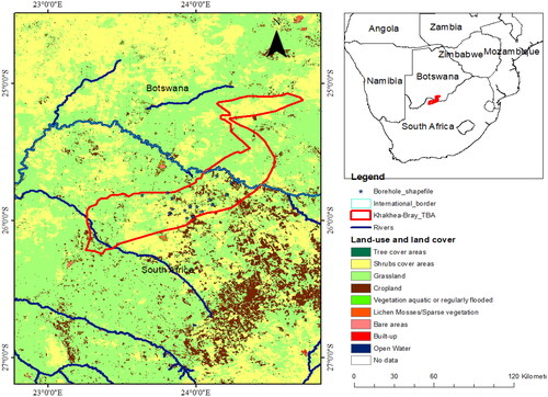
Khakea–Bray transboundary aquifer region covers approximately 3000 km² (Turton et al. 2006). The area is characterised by semiarid environment due to the low rainfall received (Godfrey and Van Dyk 2002). It receives low annual rainfall of an average of approximately 300–450 mm per year (Turton et al. 2006; Altchenko and Villholth 2013; Haasbroek 2018). It is also characterised by a mean annual catchment evapotranspiration of 2107 mm per year (Haasbroek 2018). Additionally, the area is characterized by very low (0–2 mm per year) to low (2–20 mm per year) annual recharge (Turton et al. 2006). Recharge results from infiltration through the beds of perennial from run-off to closed depressions, swamps and pans (Carlsson et al. 2009).

The human population density residing in the Khakea–Bray transboundary aquifer region is approximately 57,000. Most of activities are dependent on groundwater including farming (i.e. subsistence and commercial) and ranching livestock (Godfrey and van Dyk 2002; Turton et al. 2006). It was estimated that a mean annual amount of 1.4 mm³ of groundwater was abstracted in South Africa side during the year 2010 (Transboundary Waters Assessment Programme Groundwater 2015). This might have impacts on GDEs found in Khakea–Bray transboundary aquifer region.

2.2. Data acquisition and processing

2.2.1. Satellite images and preprocessing

Sentinel-2 MSI images were acquired in October 2020 with 10 m resolution was acquired from Google Earth Engine (GEE) platform (https://code.earthengine.google.com). The image was acquired at the end of dry season (October 2020) following the criterion that vegetation that remain green in dry season have access to groundwater (Barron et al. 2014). It was further corrected for geometric and atmospheric errors. Sentinel-2 imagery was selected based on its historical success in vegetation, water and GDEs mapping, assessment and monitoring (Kaplan and Avdan 2017; Ludwig et al. 2019; Chiloane et al. 2022). Frequency of revisit time and spatial resolution also guided the use of Sentinel-2 in this study. With this criterion, Sentinel-2 image of the dry season were used to calculate all the spectral indices. According to National Aeronautics and Space Administration (NASA) (https://power.larc.nasa.gov/data-access-viewer/) our study area received the lowest rainfall average of 0.15 mm for dry season (April to October) where October received 0.40 mm when compared wet season (January to March and November to December) with average of 2.2 mm in 2020 experienced a low rainfall.

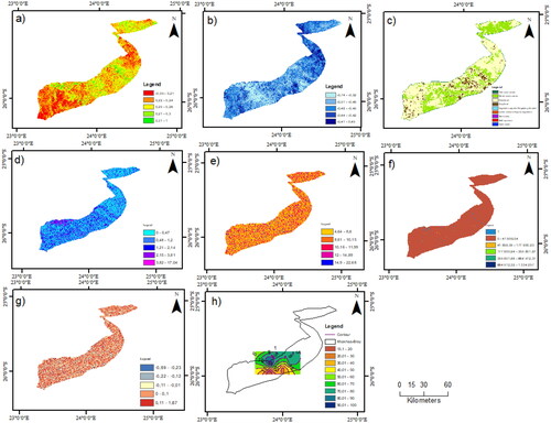
Seven thematic layers, namely, NDVI, MNDWI, LULC, slope, TWI, curvature and flow accumulation were prepared to assess the GDEs with the aid of remote sensing and GIS techniques. These variables are considered to influence groundwater dependence of ecosystems (Duran-Llacer et al. 2021; Liu et al. 2021). Martínez-Santos et al. (2021) also added that the preferred variables should be selected on a case-specific. In this case the parameters for this study were selected taking into account that the potential indicators of GDEs are vegetation communities. Figure 2 illustrate an overview of the adopted methodology.

Figure 2. Spatial distribution of explanatory variables, (a) NDVI; (b) MNDWI; (c) LULC; (d) Slope; (e) TWI; (f) Flow accumulation; (g) Curvature; (h) GWL.

Satellite observations reveal potential information about the presence of GDEs particularly in arid and semiarid environments (Liu et al. 2021). This is usually captured by vegetation and water related indices like the NDVI, Enhanced Vegetation Index (EVI), Ratio Vegetation Index (RVI) and Normalised Difference Water Index (NDWI), MNDWI, Automated Water Extraction Index (AWEI) and Water Ratio Index (WRI) (Pérez Hoyos et al. 2016; Chiloane et al. 2020). In this study, NDVI was used as a proxy for vegetation productivity (Glanville et al. 2016; Fontana and Collischonn 2019), whereas MNDWI was used to determine the presence of moisture content in the area (Glanville et al. 2016; Sarun et al. 2016).

The NDVI is widely used and is considered appropriate for arid region settings because studies found that exceptionally high biomass conditions are not encountered within the arid areas (Petus et al. 2013, Huntington et al. 2016). Furthermore, it has been used in various studies to identify terrestrial ecosystems and wetlands that depend on groundwater (Barron et al. 2012; Barron et al. 2014; White et al. 2016; Santos; Duran-Llacer et al. 2021). MNDWI has also been successfully used in the delineation of surface water features (Nhamo et al. 2017; Masocha et al. 2018; Chiloane et al. 2020; Orimoloye et al. 2020). Thus, these indices were used in this study based on their well delineation performance in the arid and semiarid environments (Biswas et al. 2020; Duran-Llacer et al. 2021; Chiloane et al. 2022).

The vegetation index (NDVI) and water index (MNDWI) were obtained by the following equations using the map algebra tool from the spatial analyst tools in ArcMap 10.8 (1) $$\mathrm{NDVI}=\frac{\mathrm{NIR}-\mathrm{R}}{\mathrm{NIR}+\mathrm{R}}$$(1) (2) $$\mathrm{MNDWI}=\frac{\mathrm{G}-\mathrm{SWIR}1}{\mathrm{G}+\mathrm{SWIR}1}$$(2) where R — red band (Band 4), NIR — near infrared (Band 8), G — green (Band 3) and SWIR1 — short-wave infrared (Band 11).

Shuttle Radar Topography Mission (SRTM) void-filled image, with 30 m spatial resolution, was downloaded from USGS online portal (https://earthexplorer.usgs.gov/). The downloaded SRTM was used to extract information about explanatory variables include slope, curvature, flow accumulation and TWI of the study area in ArcGIS 10.8 software. Slope and related parameters such as curvature, TWI are predicted to explain the areas where GDEs occurs as they control accumulation of water (Martínez-Santos et al. 2021). TWI map was used also as the integrator of soil properties since its computation sums up the influence of topographic roughness, hillslope and foothill on sideways groundwater flow. Thus, areas of high TWI allow the identification of areas of soil moisture accumulation and infiltration potential (Owolabi et al. 2020). Duran-Llacer et al. (2021) further emphasised that TWI demonstrates soil moisture conditions. For instance, Biswas et al. (2020) and Kumar et al. (2022) indicated that slope plays a dominant role in determining run-off and the rate of infiltration, thus, the gentle the slope the more infiltration and groundwater recharge which assures the presence of GDEs. Martínez-Santos et al. (2021) further indicated that GDEs usually occur in valleys and depressions, where the water table intersects the topographic surface. This implies that both topography and the elevation of the water table are likely predictors for GDEs occurrence. Thus, geomorphology of an area is considered essential component in delineation of GDEs (Biswas et al. 2020).

LULC data for the year 2016 were obtained from the European Space Agency (ESA) prototype land cover map of Africa version 1.0 based on one year of Sentinel-2A observation from December 2015 to December 2016 (http://2016africalandcover20m.esrin.esa.int/download.php?token=e23ee4b5a8858e70730e0a8121efd20). The downloaded land cover map comprises the 20 m resolution and ten primary land cover classes, including trees cover areas, shrub cover areas, grassland, cropland, vegetation aquatic or regularly flooded, sparse vegetation, bare areas, built-up areas, ice/snow (does not exist in South Africa and Botswana) and open water. LULC data was used in this study since Biswas et al. (2020) indicated that the importance on infiltration, surface water and groundwater requirements can be inferred from land cover map of an area of interest. Thus, LULC influences the occurrence of groundwater (Kumar et al. 2022).

Groundwater level data for this study was obtained from Southern African Development Community-Groundwater Information Portal (SADC-GIP) (http://www.gip.sadc-gmi.org/). Twenty-two boreholes information were used for validation of derived GDEs map. Rainfall data for October 2020 was acquired from Center for Hydrometeorology and Remote Sensing (CHRS) (https://chrsdata.eng.uci.edu/). The data has resolution of 0.04° × 0.04° or 4 km × 4 km. All the downloaded data datasets Sentinel-2, Land cover map, DEM and rainfall data were extracted for the study area and resampled to 30 m using bilinear method to ensure high quality results. They were also re-projected to the WGS 1984 UTM Zone 34S geographical coordinates system.

2.2.2. Classification

The NDVI and MNDWI were classified in ArcMap 10.8 and resulted into five classes. The class five represented the highly productive vegetation and surface water associated with water availability for NDVI and MNDWI respectively. Class one to four are characterised with vegetation and water bodies that have limited access to groundwater whereas class five represented the areas with the highest potential for GDEs. Vegetation that are productive and the presence of surface water in prolonged dry period indicate that they have access to groundwater resources (Dresel et al. 2010; Barron et al. 2014; Gonzalez et al. 2019).

All other explanatory variables were also produced with five classes (i.e. one to five), except for LULC and groundwater level with ten and nine classes, respectively (Figure 2). The maps were reclassified into two classes, namely, class one represented areas that were characterised by highly productive vegetation, high moisture, natural vegetation, gentle slopes of less than 3%, positive curvature (depression areas), high flow accumulation and TWI and shallow groundwater level depth, while class two represent areas that do not have suitable characteristics to support GDEs (Figure 5).

Land cover that are not suitable for GDEs existence including cropland, bare areas and built-up areas and suitable landcover types such as trees cover areas, shrub cover areas, grassland, vegetation aquatic or regularly flooded, sparse vegetation and open water. The topographic characteristics that were calculated from SRTM dataset were selected based on the criteria suitable for GDEs. They were set as areas with a gentle slope of less or equal to 3%, a positive curvature values and very high values of TWI and flow accumulation, as suitable for GDEs occurrence. Steep slope with value greater than 3, curvature with negative values and, TWI and flow accumulation with fewer values were categorised as nonsuitable for GDEs occurrence. Figure 2 illustrate the spatial distribution of explanatory variables used in this study.

2.2.3. Weight calculation

Weights were respectively assigned to the various thematic layers depending on their extent of influence on the GDEs delineation (i.e. NDVI, MNDWI, LULC, slope, TWI, curvature and flow accumulation) using AHP techniques. Analytical hierarchical process was used in this study since it has been rated as the most efficient multicriteria decision-making tool (Jha et al. 2010). The relative importance of the used explanatory variables was determined using Saaty’s (1980) AHP method based on a scale of 1–9 (Table 1) as stated in Goepel, (2013). Furthermore, a paired-wise comparison matrix was developed to compare all the explanatory variables and their influence on GDEs by assigning specific values to these explanatory variables (Table 2). All seven explanatory variables were integrated using weighted overlay tool in GIS environment to produce GDEs map with consistency ratio of 0.075.

Table 1. Class ratings and weights of explanatory variables in groundwater-dependent ecosystem (GDE) delineation.

Explanatory variable	Unit	Class	GDEs suitability	Class ratings	Weight (%)	Consistency measure
NDVI	Level	–0.05 − 0.21	Not suitable	2	26.4	12.6
		0.21 − 0.24
		0.24 − 0.26
		0.26 − 0.30
		0.30 − 1	Suitable	1
MNDWI	Level	–0.74 to −0.52	Not suitable	2	18.1	8.9
		–0.52 to −0.49
		–0.49 to −0.45
		–0.45 to −0.42
		–0.42 − 0.45	Suitable	1
LULC	Level	Unknown	Not suitable	2	25.0	5.6
		Built up areas
		Bare areas
		Cropland
		Vegetation aquatic or regularly flooded	Suitable	1
		Lichen Mosses/ Sparse vegetation
		Shrubs cover areas
		Tree cover areas
		Open water
		Grassland
Slope	%	0 − 0.47	Suitable	1	10.2	4.4
		0.47 − 1.20
		1.20 − 2.14
		2.14 − 3.81
		3.81 − 17.04	Not suitable	2
TWI	Level	4.64 − 8.60	Not suitable	2	9.1	3.3
		8.60 − 10.15
		10.15 − 11.99
		11.99 − 14.89
		14.89 − 22.68	Suitable	1
Flow accumulation	m	0–41 859.04	Not suitable	2	7.7	3.6
		41 859.04–177 900.93
		177 900.93–355 801.87
		355 801.87–664 512.31
		664 512.31 − 1 334 257	Suitable	1
Curvature	m	–0.89 to −0.23	Not suitable	2	3.6	1.1
		–0.23 to −0.12
		–0.12 to −0.01
		–0.01 − 0.10
		0.10 − 1.67	Suitable	1

Table 2. Pair-wise comparison matrix of seven explanatory variables.

Explanatory variables	NDVI	MNDWI	LULC	Slope	TWI	Flow accumulation	Curvature	Normalized principal Eigenvector (%)	Final consistency measure (%)
NDVI	1	1	1	1	5	5	9	25.94	11.2
MNDWI	1	1	1	3	1	1	5	17.81	8.0
LULC	1	1	1	3	3	5	7	25.28	5.9
Slope	1	1/3	1/3	1	1	1	3	10.34	6.2
TWI	1/5	1	1/3	1	1	1	3	9.18	3.6
Flow accumulation	1/5	1	1/5	1	1	1	1	7.76	4.4
Curvature	1/9	1/5	1/7	1/3	1/3	1	1	3.68	1.6
Consistency Ratio (CR) − 0.075
Consistency Index (CI) − 0.09
Random Index (RI) − 1.32
Principal Eigen values − 7.603

2.2.4. Validation and statistical analysis

Derived GDEs map was validated with the GWL data from the 22 boreholes, rainfall data and LULC data within the study area. The coefficient of determination (r²), coefficient of correlation (r) and the p-value of the relationship between GDEs and groundwater data from boreholes and rainfall were calculated in Microsoft Excel, while with LULC was calculated in Arc GIS environment. The correlation coefficient (r) is a measure of the strength of a linear relationship between two variables (Liu et al. 2021). The GDEs that occurred in areas with shallow GWL (less than 20 m), indicate the reliability of the results. This is based on one of the assumptions that has been used for the validation of GDE identification that assume that an ecosystem depends on the presence of shallow groundwater, within the rooting depth (Eamus and Froend 2006; Liu et al. 2021).

The groundwater level has been presented in the form of contours (Figure 2h). The study used interpolation approach to groundwater elevations at monitoring wells to get groundwater elevation contours across the landscape (Figure 2h). This is regarded as more accurate approach since it provides much more accurate contours of depth-to-groundwater along streams and other land surface depressions where GDEs are commonly found. Unlike the common practice of contour depth-to-groundwater over a large area by interpolating measurements at monitoring wells. This practice causes errors when the land surface contains features like stream and wetland depressions because it assumes the land surface is constant across the landscape and depth-to-groundwater is constant below these low-lying areas.

In addition, GDEs have been associated with boreholes by applying a 5 km buffer ring around the boreholes. LULC dataset was also used for GDEs validation. Percentage of the GDEs were calculated within each LULC type that has the potential to support GDEs. This was conducted in ArcGIS environment (Figure 3).

Figure 3. Flow diagram summarising the methodological and analysis steps for mapping groundwater-dependent ecosystem (GDE) distribution.

2.3. Results

2.3.1. Suitability classes for GDE from explanatory variables

The NDVI (vegetation index) shows that northern, central and south-western part of the study has high vegetation productivity when compared to the other regions. The study area was characterised by gentle slopes except for sections of the south-western part where mountains are found. The curvature (surface depression) and TWI are evenly spread and indicate that there is little water flowing within the study area. The MNDWI (water index) demonstrated the presence of surface water on the northern, north-eastern, central and sparsely distributed on the southern part of the study area.

Natural vegetation dominates the area and according to the land cover data, the areas of natural vegetation consist of grassland; trees cover area, shrub cover areas, vegetation aquatic or regularly flooded and sparse vegetation. Thus, our analysis showed that a small proportion of areas in Khakea–Bray transboundary aquifer region has the potential to support GDEs. The areas in green colour are characterised by highly productive vegetation, high moisture, natural and productive vegetation, gentle slopes of less than 3% which will accommodate GDEs that occurs on the bottom valleys, positive curvature (depression areas), high flow accumulation and TWI and shallow GWL, thus suitable to identify the presence of GDEs. Areas indicated by the peach colour do not have suitable characteristics to classify the occurrence of GDEs (Figure 4).

Figure 4. Individual map derived from (a) NDVI; (b) MNDWI; (c) LULC; (d) Slope; (e) TWI; (f) Flow accumulation; (g) Curvature; (h) GWL showing areas that are suitable and unsuitable for GDE mapping.

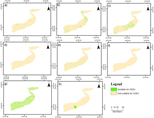
The GDEs map of the study area was derived through the integration of all the classified suitable explanatory variables in GIS environment and is it shown in Figure 5. The GDEs are sparsely distributed and dominant in the central part along the river and south-western part (mountainous) when compared to the other areas where they are sparsely spread. The GDEs covers small total area of 7219.08 hectares (ha) when compared to the huge total area covered by non-GDEs of 530,328.51 ha (Table 3).

2.3.2. The distribution of GDEs in the Khakea–Bray transboundary aquifer

Figure 5. Distribution of GDE within the Khakea–Bray transboundary aquifer region derived from integrated explanatory variables.

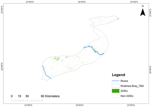
Table 3. GDEs category and their distribution.

Category	Area (km^2)	Area (ha)	Percentage (%)
GDEs	721.91	7219.08	1.34
Non-GDEs	53032.85	530328.51	98.66

2.3.3. Validation of GDEs map

2.3.3.1. Validation with groundwater level data

The GWL data obtained from SADC-GIP related to the 22 groundwater boreholes distributed in the study area were used to validate the mapped GDEs (Figure 6). The level depth of the groundwater in the study area ranges from 13.74 m to 93.68 m below ground level. The GDEs that falls within shallow GWL (less than 20 m) covers a total area of 1.44 km² (6.32%) whereas those that falls within deep GWL covers 21.33 km² (93.68%) (Figure 7). The results indicate that a large portion of the study area in deep GWL support GDEs occurrence. Furthermore, the data shows that all of the boreholes (22) used for validation exist in the Non-GDEs (Table 4).

Figure 6. GDE map of the Khakea–Bray transboundary aquifer and borehole locations.

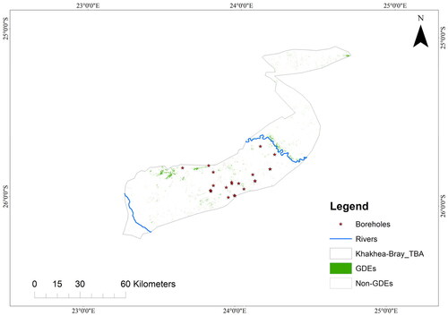
Figure 7. (a) Areas identified as GDE with shallow GWL (less than 20 m) and deep GWL (larger than 20 m) and (b) the area and percentage of GDEs in GWL.

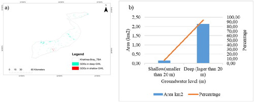
Table 4. The data of groundwater boreholes located in the Khakea–Bray transboundary aquifer region.

No.	Station name	Date	Coordinate (WSG 84)		Water level (m, bgl)	GDEs map classes^a
			X	Y
1	D4N1703	2020/02/12	23.63695	–25.81278	61.9	2
2	D4N2326	2020/09/09	23.98139	–25.97056	29.72	2
3	D4N2325	2020/09/09	23.98417	–25.9725	28.59	2
4	D4N2323	2020/09/10	23.80765	–25.79589	90.82	2
5	D4N2322	2020/09/09	23.94156	–25.98289	28.51	2
6	D4N2320	2020/11/27	23.839	–25.83446	93.68	2
7	D4N2317	2020/09/09	23.92636	–25.92356	46.45	2
8	D4N2316	2020/09/08	23.82593	–25.94892	13.74	2
9	D4N2315	2020/09/07	24.09883	–25.84426	75.16	2
10	D4N2314	2020/09/08	24.11524	–25.88143	84.76	2
11	D4N2311	2020/09/07	24.2113	–25.8077	69.41	2
12	D4N2310	2020/09/07	24.11333	–25.88194	22.71	2
13	D4N2305	2020/09/08	24.00768	–25.89818	22.29	2
14	D4N2302	2020/09/10	24.04289	–25.93098	35.42	2
15	D4N2298	2020/09/07	24.2116	–25.8089	70.98	2
16	D4N2297	2020/09/07	24.23915	–25.72107	70.88	2
17	D4N2296	2020/09/08	24.14435	–25.67413	81.19	2
18	D4N2291	2020/09/08	23.8249	–25.9429	11.7	2
19	D4N2290	2020/09/08	23.82339	–25.94431	10.13	2
20	D4N2289	2020/09/08	23.8418	–25.9138	36.32	2
21	D4N2288	2020/09/09	23.9625	–25.8997	29.18	2
22	D4N2287	2020/09/09	23.9616	–25.8918	47.53	2

^a The classes of the derived GDEs by GIS with AHP for Khakea–Bray Transboundary Aquifer.

bgl: below ground level.

A spearman’s correlation analysis results demonstrated strong positive significant correlation (r = 0.67; p = 0.00; r² = 0.45) between the borehole data and GDEs classes (Table 5). These results indicate a possible delineation of GDEs in the study area using remote sensing and GIS techniques along with AHP. Additionally, the GDEs within 5 km buffer covers a total area of 85,257 ha (0.97%) (Figure 8).

Figure 8. Association of GDEs to boreholes within 5 km buffer in Khakea–Bray transboundary aquifer.

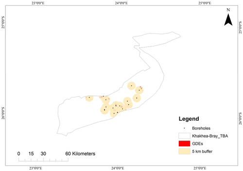
Table 5. Results of the GDEs model assessment with groundwater level data.

Test parameters	Estimates
Correlation coefficient (r)	0.67
Coefficient of determination (r^2)	0.45
t value	24,14138222
Degree of freedom	704
p value	2,79375 E – 94

2.3.3.2. Validation with land cover types

LULC data was also used to validate the GDEs map. In areas that have the potential to support the occurrence of GDEs, the percentage was determined of each landcover type that is suitable for GDEs (Table 6). Each type of LULC was overlay weighted with GDEs in ArcGIS environment to obtain area covered by GDEs within each LULC types. The results demonstrated that GDEs were associated with grasslands and shrublands. Shrublands were recognised as the landcover type most likely to access groundwater covering 23.58 ha of the area (53.27%), followed by grassland covering 18.90 (42.66%), while vegetation aquatic or regularly flooded was the least likely covering less than 0.01 ha of the area.

Table 6. Areas and percentages of the GDEs for each LULC type.

GDEs covered in different land covers	Area (km^2)	Area (ha)	Percentage
Trees cover	0.10	0.99	2.26
Shrubland	2.36	23.58	53.27
Grassland	1.89	18.90	42.66
Regularly flooded	<0.01	<0.10	<0.00
Lichen Mosses/ sparse vegetation	0.06	0.63	1.35
Water	0.03	0.27	0.45

2.3.3.3. Validation with rainfall data

Rainfall data was used to verify the accuracy of GDEs mapping. The spatial distribution was obtained using the ordinary Kriging interpolation method (Figure 9). The monthly rainfall ranges from 15.27 to 64.76 mm per month with more rainfall received from northern and some region of southern and south western part of the area. The coefficient of determination (r² = 0.49) obtained indicates that the GDEs model is partially fit for the delineation of GDEs. This was further established by the coefficient of correlation (r = 0.70) and the test for significance (p = 0.00) for the model which that the modelling procedure shows a very significant and strong positive relationship with the borehole data (Table 7). This indicate that the model can provide relevant and applicable information on the availability of groundwater in dwelling of boreholes.

Figure 9. Spatial pattern of the trend for month rainfall over October 2020 in Khakea–Bray transboundary aquifer.

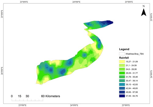
Table 7. Results of the GDEs model assessment with rainfall data.

Test parameters	Estimates
Correlation coefficient (r)	0.70
Coefficient of determination (r^2)	0.49
t value	26,01186038
Degree of freedom (df)	704
p value	4,6994 E – 105

2.4. Discussion

2.4.1. Distribution of GDEs in Khakea–Bray transboundary aquifer region

Identification and delineation of GDEs is a crucial step towards sustainable groundwater resource use and GDEs since groundwater resources are being increasingly depended upon under a warming climate. The delineation of GDEs was prepared for the study area due to the necessity to understand and improve groundwater management practices in the area. Based on this, our study area was categorised into two classes, where class one represented GDEs and two represent non-GDEs. The non-GDEs covers about 530,328.51 ha which accounts for 98.66%, whereas GDEs covers 7219.08 ha which accounts for 1.34% of the transboundary area. The GDEs of this study covers a small portion of the area when compared to other studies (Marques et al. 2019; Duran-Llacer et al. 2021; Liu et al. 2021) where their GDEs covers large portion than non-GDEs. However, the study is similar to Xu et al. (2022) where their study found that GDEs covers small percentage of their areas when compared areas covered by non-GDEs.

The results of the study indicate that the GDEs are sparsely, although unevenly distributed across Khakea–Bray transboundary aquifer. The GDEs were primarily concentrated in the northern, central and south-western part where groundwater discharge may be expected. Due to limited knowledge on amount of groundwater used by the vegetation in the area, the ecosystems particularly in the central part might be reliant on the groundwater recharged by the Molopo River. This results are similar to Liu et al. (2021) where they found that the potential GDEs were concentrated primarily around large lakes, where groundwater discharge may be expected. Similarly, Duran-Llacer et al. (2021) indicated the very high GDEs zone mainly in the river valleys and flat zones where there is significant interaction between surface and groundwater.

The northern and central parts were characterised by a gentle slope and fall within natural vegetation particularly shrubland and grassland. This is not surprising as Biswas et al. (2020) and Kumar et al. (2022) declared the importance of gentle slope in influencing less run-off and more infiltration rate, and groundwater recharge which promises the presence of GDEs. Additionally, Marques et al. (2019) found that slope is one of the factors influencing the occurrence of groundwater dependent vegetation in administrative region of Alentejo, Portugal. Duran-Llacer et al. (2021) also found that very high and high GDEs zone were located on flat terrain for 2002 and 2017 in semienvironments in Chile.

According to the LULC map of the study, shrubland and grassland covers 57.28% and 35.97% of the area respectively, accounting for 93.25% of the area combined. The derived GDEs map demonstrate that GDEs are mostly found in the shrubland with total area of 23.58 ha (53.27%) and 18.9 ha (42.66%) in grassland than other LULC types suitable for GDEs occurrence. This is similar to Liu et al. (2021) where they have noticed that areas of grassland in certain areas had high potential GDEs. Similarly, Brim Box et al. (2022) indicated that large trees (e.g. Corymbia spp.) that were considered groundwater dependent in the study area occur as small, discrete clusters in hummock grassland. It is reasonable that the GDEs are distributed mainly on grassland and shrubland since our study took place in Savanna Biome that is dominated by grass and shrubs (Low and Rebelo 1996) on a gentle slope.

The grassland of which GDEs were found was dominated by Eragrostis lehmanniana that prefer areas where minimum winter temperatures rarely fall below 0 °C and summer rainfall is between 150 mm and 220 mm (Uchytil 1992). Their basal leaves stay evergreen throughout the winter and stems stay green after autumn frost (Bosch et al. 2002). This might be owing to access to groundwater by the species. On the other side, shrubland that dominates the study area is Grewia flava (Weare and Yalala 1971; Mpakairi et al. 2022). Grewia flava is favoured by the semiarid climate that is characterised by hot summers and arid cool winters. It is also dominant in areas with rainfall that is averaging about 350 mm annually (Mainah 2001).

Surface water systems are scarcely distributed in Khakea–Bray transboundary aquifer region as shown in Figure 4, with only 2 main rivers, namely, Molopo River in the central part and Phepane River in the southern part of the area. Molopo River which cut across the central region might be affected by groundwater extraction due to the presence of extensive irrigation systems used mainly for potato farming (Rampheri M.B, personal observation).

In addition, the pans are common seasonally in the southern part of the areas where GDEs are sparsely distributed. Some of the pans floor are grasses which composite of species like Sporobolus spp. Eragrostis sp., Panicum coloralum, and Marsilea spp. The pans are also surrounded by species such as Acacis giraffe, Dichrostachys cinerea which are associated with topography and climate (Weare and Yalala 1971). Siebert et al. (2010) indicated that Letaba exclosures in Kruger National Park was also characterised by D. cinerea, with summer rainfall of approximately 400 mm per year and the mean daily temperature of 23.3 °C, ranging from 7.8 °C in winter, to a maximum of 34.1 °C in summer. Thus, our results indicate that the southern part is characterised by a gentle slope which might influence the pans vegetation occurrence.

2.4.2. Validation of GDEs map

Our results indicated positive significant correlation between derived GDEs map and GWL. Our results are similar to the most of the GDEs studies (Liu et al. 2021; Martínez-Santos et al. 2021) that found correlation between GDEs and GWL. This might be influenced by the presence of GDEs within shallow GWL data used in their studies. There is a theory that the more the groundwater is shallower, the higher the likelihood of GDEs (Eamus and Froend 2006; Liu et al. 2021; Xu et al. 2022). However, our study contradict with the theory since GDEs were found in the relatively deep GWL. Majority of the boreholes (21 out of 22) used for validation were characterised by deep GWL of greater than 20 m below ground level. This indicate that not all GDEs depend on shallow GWL. The results might be attributed to the root system, for example, mechanics of capillary fringe which is not well known for the study area. Furthermore, the GDEs might access the groundwater from the aquifer perches.

However, some studies (Páscoa et al. 2020) indicated the certain portion of GDEs existing in deep GWL. Marques et al. (2019) found that groundwater depth appeared to have a lower influence on groundwater-dependent vegetation density than climate drivers. On the other side, Liu et al. (2021) showed that there were some uncertainties about the assumption which may limit the validation reliability. Additionally, Hawkins et al. (2003); Wang et al. (2011); Pierret et al. (2016) indicated that the depth of vegetation roots in dry climates can sometimes reach tens of meters. Nevertheless, this suggests that accurately delineation of GDEs in semiarid environments need to be more inclusive. For example, it will need to be validated using integrated diverse methods.

Thus, rainfall data was also used to validate the precision of derived GDEs. The results indicated the strong positive significant correlation between rainfall and GDEs. This might be attributed to the principle that vegetation is positively correlated with rainfall in arid and semiarid regions. Analysis of the results of the correlation and linear regression between GDEs-GWL and GDEs-rainfall showed a significant stronger GDEs-rainfall relationship (r = 0.70) than GDEs-GWL relationship (r = 0.67). This demonstrate that the GDEs were affected more by the decrease in rainfall than by the decrease in GWL.

Overall, the results of the study indicate a possible delineation of GDEs in the study area using remote sensing and GIS techniques along with AHP techniques.

2.4.3. Strengths and limitations of GDEs mapping

Remote sensing and GIS together with in situ data show the capability to identify and delineate GDEs in the study area. The study adopted the principle that vegetation will remain green and physiologically active during extended dry periods due to access to groundwater (Tweed et al. 2007). This principle has been successfully applied in other studies (e.g. Dresel et al. 2010; Liu et al. 2021) to identify GDEs. For this study, we combined two criteria, namely, overlay analysis and correlation analysis to avoid the disadvantages of using a single criterion, an approach was adopted from Gou et al. (2015).

There is a limited number of previous studies of GDEs in transboundary aquifers in Southern Africa, thus, we proposed a combination of individual derived maps from explanatory variables, produced GDEs map from combination of all explanatory variables, and GWL. The method has produced the reliable results in identification and delineation the GDEs in Khakea–Bray transboundary aquifer region.

However, the study observed two major limitations related to classification method used for explanatory variables that were used for GDEs delineation. First, as seen from Figure 2, some areas suitable for GDEs have been exaggerated on the MNDWI map. For example, MNDWI classified some roads as surface water in the southern part and it should have been masked out because bare surface does not contain water. Similar to flow accumulation map, most of the areas have been omitted. For example, areas located on a gentle slope of less than 3% and close to water bodies like Molopo and Phepane rivers could have been covered. The quality of the GDEs delineation can be improved by investigating and including alternative water indices and topographical indices as well as machine learning algorithms and their performance.

2.5. Conclusions

Understanding the location and spatial extent of GDEs is crucial for sustainable management of groundwater resources and for their protection. Thus, adequate delineating is essential for the protection of GDEs, particularly in arid regions where GDEs are at risk of disappearing due to anthropogenic factors and changing climate. Attempts to map and delineate GDEs should always take into account the relevant explanatory variables. This study utilised method of combining two analyses (i.e. overlay analysis and correlation analysis) that are based on remote sensing datasets to identify and delineate GDEs located in Khakea–Bray transboundary aquifer region. The results of our study demonstrated the effectiveness of integrating expert opinion, GIS techniques, remote sensing and field-work for verification to suitably delineate GDEs. The coefficient of determination (r² = 0.45; r² = 0.49) obtained indicates that the GDEs model is partially fit for the delineation of GDEs. Overall, the result indicates that the approach is reliable and can be adopted for a reliable delineation of GDEs in any arid and semiarid environments.

The used approach has the potential to provide important baseline knowledge on terrestrial as well as aquatic GDEs occurrence across remote and poorly studied arid region. The validation of GDEs with rainfall and GWL confirmed the presence of GDEs in Khakea–Bray transboundary aquifer region. Thus, this study concludes that Khakea–Bray transboundary aquifer region has small proportion of area covered by GDEs, which are concentrated in the northern, central areas around the Molopo River and cultivated areas, and southern part on the foot of the mountains. The GDEs in the southern region of our study area are also sparsely distributed around the pans and Phepane River.

We further conclude that due to uncertainties and limited availability of in situ data, and observation such as vegetation root system and soil types in our study area, it was challenging to conclude on the mechanism behind the presence of GDEs in deep GWL regions. Thus, more integration of validation methods based on remote sensing is recommended in future for effective GDEs delineation studies. We also recommend further studies on the vegetation root systems with Khakea–Bray transboundary aquifer region. Better knowledge of location and spatial extent of GDEs, as well as effective implementation of groundwater management policies, should be highlighted for protecting GDEs in Khakea–Bray transboundary aquifer region to prevent their loss or destruction.

Data availability statement

Data used in this research is available upon request.

Disclosure statement

The authors declare that they have no known competing financial interests or personal relationships that could have appeared to influence the work reported in this paper.

Additional information

Funding

The authors are grateful for the financial support offered by JRS Biodiversity Foundation through the Southern African Development Community - Groundwater Management Institute (SADC-GMI). The study was also supported financially by National Research Foundation (NRF) grant number 138206 and the authors are grateful.

References

- Altchenko Y, and Villholth KG. 2013. Transboundary aquifer mapping and management in Africa: a harmonised approach. Hydrogeol J. 21(7):1497–1517.
- Barron O, Silberstein R, Ali R, Donohue R, McFarlane DJ, Davies P, Hodgson G, Smart N, Donn M. 2012. Climate change effects on water-dependent ecosystems in south-western Australia. J Hydrol. 434:95–109.
- Barron OV, Emelyanova I, Van Niel TG, Pollock D, Hodgson G. 2014. Mapping groundwater-dependent ecosystems using remote sensing measures of vegetation and moisture dynamics. Hydrol Process. 28(2):372–385.
- Biswas S, Mukhopadhyay BP, Bera A. 2020. Delineating groundwater potential zones of agriculture dominated landscapes using GIS based AHP techniques: a case study from Uttar Dinajpur district, West Bengal. Environ Earth Sci. 79(12):1–25.
- Bosch CH, Siemonsma JS, Lemmens RHMJ, and Oyen LPA. (Editors), 2002. Plant Resources of Tropical Africa / Ressources Végétales de l'Afrique Tropicale. Basic list of species and commodity grouping / Liste de base des espèces et de leurs groupes d'usage. PROTA Programme, Wageningen, the Netherlands. 341.
- Brim Box J, Leiper I, Nano C, Stokeld D, Jobson P, Tomlinson A, Cobban D, Bond T, Randall D, Box P. 2022. Mapping terrestrial groundwater‐dependent ecosystems in arid Australia using Landsat‐8 time‐series data and singular value decomposition. Remote Sens Ecol Conserv. 8(4):464–476.
- Carlsson L, Masalila-Dodo C, Bejugam R, Sola L, Alemaw BF, Mahomed I, Madec G. 2009. Groundwater review of the Molopo-Nossob Basin for rural communities including assessment of national databases at the sub-basin level for possible future integration. Fachbericht Nr. Orasecom/005/2009, 190 S.
- Chaikumbung M, Doucouliagos H, Scarborough H. 2016. The economic value of wetlands in developing countries: a meta-regression analysis. Ecol Econ. 124:164–174.
- Chiloane C, Dube T, Shoko C. 2020. Monitoring and assessment of the seasonal and inter-annual pan inundation dynamics in the Kgalagadi Transfrontier Park, Southern Africa. Phys Chem Earth, Parts A/B/C. 118:102905.
- Chiloane C, Dube T, Shoko C, 2022. Impacts of groundwater and climate variability on terrestrial groundwater dependent ecosystems: a review of geospatial assessment approaches and challenges and possible future research directions.Geocarto Intern. 37(23):6755–6779.
- Dalu T, Wasserman RJ, editors. 2021. Fundamentals of tropical freshwater wetlands: from ecology to conservation management. Elsevier.
- Doody TM, Barron OV, Dowsley K, Emelyanova I, Fawcett J, Overton IC, Pritchard JL, Van Dijk AI, Warren G. 2017. Continental mapping of groundwater dependent ecosystems: a methodological framework to integrate diverse data and expert opinion. J Hydrol: Reg Stud. 10:61–81.
- Doody TM, Hancock PJ, Pritchard JL. 2019. Information guidelines explanatory note: assessing groundwater-dependent ecosystems. Report prepared for the independent expert scientific Committee on Coal Seam Gas and Large Coal Mining development through the Department of the Environment and Energy, Common Wealth of Australia 2019.
- Dresel PE, Clark R, Cheng X, Reid M, Terry A, Fawcett J, Cochrane D. 2010. Mapping terrestrial groundwater dependent ecosystems: method development and example output. Melbourne, Australia: Department of Primary Industries.
- Dube T, Shoko C, Sibanda M, Baloyi MM, Molekoa M, Nkuna D, Rafapa B, Rampheri BM. 2020. Spatial modelling of groundwater quality across a land use and land cover gradient in Limpopo Province, South Africa. Phys Chem Earth Parts A/B/C. 115:102820.
- Duran-Llacer I, Arumí JL, Arriagada L, Aguayo M, Rojas O, González-Rodríguez L, Rodríguez-López L, Martínez-Retureta R, Oyarzún R, Singh SK. 2021. A new method to map groundwater-dependent ecosystem zones in semi-arid environments: a case study in Chile. Sci Total Environ.816:151528.
- Eamus D, Froend R. 2006. Groundwater-dependent ecosystems: the where, what and why of GDEs. Aust J Bot. 54(2):91–96.
- Eamus D, Zolfaghar S, Villalobos-Vega R, Cleverly J, Huete A. 2015. Groundwater-dependent ecosystems: recent insights from satellite and field-based studies. Hydrol Earth Syst Sci. 19(10):4229–4256.
- Erostate M, Huneau F, Garel E, Ghiotti S, Vystavna Y, Garrido M, Pasqualini V. 2020. Groundwater dependent ecosystems in coastal Mediterranean regions: characterization, challenges and management for their protection. Water Res. 172:115461.
- Fontana RB, Collischonn W. 2019. Remote sensing and GIS based analysis of Groundwater-dependent ecosystems in the Brazilian Cerrado. Simpósio Brasileiro de Recursos Hídricos (23.: foz do Iguaçu, 2019). Anais [recurso eletrônico]. Porto Alegre: ABRH.
- Ghosh S, Das A. 2020. Wetland conversion risk assessment of East Kolkata Wetland: a Ramsar site using random forest and support vector machine model. J Cleaner Prod. 275:123475.
- Glanville K, Ryan T, Tomlinson M, Muriuki G, Ronan M, Pollett A. 2016. A method for catchment scale mapping of groundwater-dependent ecosystems to support natural resource management (Queensland, Australia). Environ Manage. 57(2):432–449.
- Godfrey L, Van Dyk G. 2002. Reserve determination for the Pomfret-Vergelegen Dolomitic Aquifer, North West Province. Part of catchments D41C, D, E and F. Groundwater Specialist Report. Report No. ENV-PC 31.
- Goepel KD. 2013. Implementing the analytic hierarchy process as a standard method for multi-criteria decision making in corporate enterprises–a new AHP excel template with multiple inputs. Proceedings of the International Symposium on the Analytic Hierarchy Process, June. Kuala Lumpur, Malaysia: Creative Decisions Foundation Kuala Lumpur. Vol. 2, No. 10, p. 1–10.
- Gonzalez E, González Trilla G, San Martin L, Grimson R, Kandus P. 2019. Vegetation patterns in a South American coastal wetland using high-resolution imagery. J Maps. 15(2):642–650.
- Gou S, Gonzales S, Miller GR. 2015. Mapping potential groundwater‐dependent ecosystems for sustainable management. Ground Water. 53(1):99–110.
- Gronwall J, Danert K. 2020. Regarding groundwater and drinking water access through a human rights lens: self-supply as a norm. Water. 12:419.
- Gxokwe S, Dube T, Mazvimavi D. 2020. Multispectral remote sensing of wetlands in semi-arid and arid areas. A review on applications, challenges and possible future research directions. Remote Sens. 12(24):4190.
- Haasbroek 2018. Khakea-Bray Transboundary Dolomite Aquifer Recharge Assessment. Available at: https://wis.orasecom.org/khakheabrayaquifer/.
- Hawkins BA, Field R, Cornell HV, Currie DJ, Guégan J-F, Kaufman DM, Kerr JT, Mittelbach GG, Oberdorff T, O'Brien EM, et al. 2003. Energy, water, and broad‐scale geographic patterns of species richness. Ecology. 84(12):3105–3117.
- Howard J, Merrifield M. 2010. Mapping groundwater dependent ecosystems in California. PLoS One. 5(6):11249.
- Huntington J, McGwire K, Morton C, Snyder K, Peterson S, Erickson T, Niswonger R, Carroll R, Smith G, Allen R. 2016. Assessing the role of climate and resource management on groundwater dependent ecosystem changes in arid environments with the Landsat archive. Remote Sens Environ. 185:186–197.
- Jha MK, Chowdary VM, Chowdhury A. 2010. Groundwater assessment in Salboni Block, West Bengal (India) using remote sensing, geographical information system and multi-criteria decision analysis techniques. Hydrogeol J. 18(7):1713–1728.
- Kaplan G, Avdan U. 2017. Mapping and monitoring wetlands using Sentinel-2 satellite imagery. ISPRS annals of photogrammetry. Remote Sens Spatial Infor Sci. 4:1–7.
- Kibler CL, Schmidt EC, Roberts DA, Stella JC, Kui L, Lambert AM, Singer MB. 2021. A brown wave of riparian woodland mortality following groundwater declines during the 2012–2019 California drought. Environ Res Lett. 16(8):084030.
- Kløve B, Ala-Aho P, Bertrand G, Boukalova Z, Ertürk A, Goldscheider N, Ilmonen J, Karakaya N, Kupfersberger H, Kvœrner J, et al. 2011. Groundwater dependent ecosystems. Part I: hydroecological status and trends. Environ Sci Policy. 14(7):770–781.
- Koit O, Tarros S, Pärn J, Küttim M, Abreldaal P, Sisask K, Vainu M, Terasmaa J, Retike I, Polikarpus M. 2021. Contribution of local factors to the status of a groundwater dependent terrestrial ecosystem in the transboundary Gauja-Koiva River basin, North-Eastern Europe. J Hydrol. 600:126656.
- Kuginis L, Dabovic J, Byrne G, Raine A, Hemakumara H. 2016. Methods for the identification of high probability groundwater dependent vegetation ecosystems. DPI Water. Sydney: NSW.
- Kumar A, Kanaujia A. 2014. Wetlands: significance. Threats and their conservation. Environment. 7:1–24.
- Kumar M, Singh SK, Kundu A, Tyagi K, Menon J, Frederick A, Raj A, Lal D. 2022. GIS-based multi-criteria approach to delineate groundwater prospect zone and its sensitivity analysis. Appl Water Sci. 12(4):1–14.
- Liu C, Liu H, Yu Y, Zhao W, Zhang Z, Guo L, Yetemen O. 2021. Mapping groundwater-dependent ecosystems in arid Central Asia: implications for controlling regional land degradation. Sci Total Environ. 797:149027.
- Low AB, Rebelo AG. 1996. Vegetation of South Africa, Lesotho and Swaziland. Pretoria: department of Environmental Affairs and Tourism. Voelcker Bird Book Fund. calvus in relation to rainfall and grass-burning. IBIS. 127:159–173.
- Ludwig C, Walli A, Schleicher C, Weichselbaum J, Riffler M. 2019. A highly automated algorithm for wetland detection using multi-temporal optical satellite data. Remote Sens Environ. 224:333–351.
- Mainah J. 2001. The distribution and association of Grewia flava with other species in the Kalahari environment. Botswana Notes Rec. 33(1):115–128.
- Majola K, Xu Y, Kanyerere T. 2021. Assessment of climate change impacts on groundwater-dependent ecosystems in transboundary aquifer settings with reference to the Tuli-Karoo transboundary aquifer. Ecohydrol Hydrobiol. 22(1):126-140.
- Mango N, Siziba S, Makate C. 2017. The impact of adoption of conservation agriculture on smallholder farmers’ food security in semi-arid zones of southern Africa. Agric Food Secur. 6(1):1–8.
- Marques IG, Nascimento J, Cardoso RM, Miguéns F, de Melo MTC, Soares PM, Gouveia CM, Besson CK. 2019. Mapping the suitability of groundwater-dependent vegetation in a semi-arid Mediterranean area. Hydrol Earth Syst Sci. 23(9):3525–3552.
- Martínez-Santos P, Díaz-Alcaide S, De la Hera-Portillo A, Gómez-Escalonilla V. 2021. Mapping groundwater-dependent ecosystems by means of multi-layer supervised classification. J Hydrol. 603:126873.
- Masocha M, Dube T, Makore M, Shekede MD, Funani J. 2018. Surface water bodies mapping in Zimbabwe using landsat 8 OLI multispectral imagery: a comparison of multiple water indices. Phys Chem Earth, Parts A/B/C. 106:63–67.
- Miller GR, Chen X, Rubin Y, Ma S, Baldocchi DD. 2010. Groundwater uptake by woody vegetation in a semiarid oak savanna. Water Resour Res. 46(10):1–14.
- Mpakairi KS, Dube T, Dondofema F, Dalu T. 2022. Spatio–temporal variation of vegetation heterogeneity in groundwater dependent ecosystems within arid environments. Ecol Inf. 69:101667.
- Münch Z, Conrad J. 2007. Remote Sensing and GIS base determination of groundwater dependent ecosystems in the Western Cape, South Africa. Hydrogeol J. 15(1):19–28.
- Nhamo L, Magidi J, Dickens C. 2017. Determining wetland spatial extent and seasonal variations of the inundated area using multispectral remote sensing. WSA. 43(4):543–552.
- Orellana F, Verma P, Loheide SP, Daly E. 2012. Monitoring and modeling water‐vegetation interactions in groundwater‐dependent ecosystems. Rev Geophys. 50(3):1–24
- Orimoloye IR, Kalumba AM, Mazinyo SP, Nel W. 2020. Geospatial analysis of wetland dynamics: wetland depletion and biodiversity conservation of Isimangaliso Wetland, South Africa. J King Saud Univ-Sci. 32(1):90–96.
- Owolabi ST, Madi K, Kalumba AM, Orimoloye IR. 2020. A groundwater potential zone mapping approach for semi-arid environments using remote sensing (RS), geographic information system (GIS), and analytical hierarchical process (AHP) techniques: a case study of Buffalo catchment, Eastern Cape, South Africa. Arab J Geosci. 13(22):1–17.
- Páscoa P, Gouveia CM, Kurz-Besson C. 2020. A simple method to identify potential groundwater-dependent vegetation using NDVI MODIS. Forests. 11(2):147.
- Pérez Hoyos IC, Krakauer NY, Khanbilvardi R, Armstrong RA. 2016. A review of advances in the identification and characterization of groundwater-dependent ecosystems using geospatial technologies. Geosciences. 6(2):17.
- Petus C, Lewis M, White D. 2013. Monitoring temporal dynamics of Great Artesian Basin wetland vegetation, Australia, using MODIS NDVI. Ecol Indic. 34:41–52.
- Pierret A, Maeght JL, Clément C, Montoroi JP, Hartmann C, Gonkhamdee S. 2016. Understanding deep roots and their functions in ecosystems: an advocacy for more unconventional research. Ann Bot. 118(4):621–635.
- Rapinel S, Fabre E, Dufour S, Arvor D, Mony C, Hubert-Moy L. 2019. Mapping potential, existing and efficient wetlands using free remote sensing data. J Environ Manage. 247:829–839.
- Rohde MM, Froend R, Howard J. 2017. A global synthesis of managing groundwater dependent ecosystems under sustainable groundwater policy. Ground Water. 55(3):293–301.
- Rohde MM, Stella JC, Roberts DA, Singer MB. 2021. Groundwater dependence of riparian woodlands and the disrupting effect of anthropogenically altered streamflow. Proc Natl Acad Sci USA. 118(25):e2026453118
- Saaty TL. 1980. The analytic hierarchy process, planning, priority setting, resource allocation. New York: McGraw-Hill. p. 287.
- Saito L, Christian B, Diffley J, Richter H, Rohde MM, Morrison SA. 2021. Managing groundwater to ensure ecosystem function. Ground Water. 59(3):322–333.
- Sarun S, Vineetha P, Kumar RA. 2016. Semi-automated methods for wetland mapping using Landsat ETM+: a case study from tsunami affected panchyats of Alappad & Arattupuzha, South Kerala. Int J Sci Res. 5(8):1150–1154.
- Siebert F, Siebert SJ, Eckhardt HC. 2010. The vegetation and floristics of the Letaba exclosures, Kruger National Park, South Africa. Koedoe. 52(1):1–12.
- Thamaga KH, Dube T, Shoko C. 2021. An assessment of small wetland ecohydrological dynamics using Sentinel-2 MSI derived spectral indices in semi-arid environments of South Africa.
- Tian S, Zhang X, Tian J, Sun Q. 2016. Random forest classification of wetland landcovers from multi-sensor data in the arid region of Xinjiang, China. Remote Sens. 8(11):954.
- Transboundary Waters Assessment Programme Groundwater. 2015. Transboundary Aquifer Information Sheet. AF6-Khakhea/Bray Dolomite.
- Turton A, Godfrey L, Julien F, Hattingh H. 2006. Unpacking groundwater governance through the lens of a trialogue: a Southern African case study. International Symposium on Groundwater Sustainability (ISGWAS), Alicante, Spain. p. 24–27.
- Tweed SO, Leblanc M, Webb JA, Lubczynski MW. 2007. Remote sensing and GIS for mapping groundwater recharge and discharge areas in salinity prone catchments, southeastern Australia. Hydrogeol J. 15(1):75–96.
- Uchytil RJ. 1992. Eragrostis lehmanniana. In: Fire effects information system (Online), USDA Forest Service.
- Verlicchi P, Grillini V. 2020. Surface and groundwater quality in South Africa and Mozambique-Analysis of the most critical pollutants for drinking purposes and challenges in water treatment. Water. 12:305.
- Wang Y, Shao MA, Zhu Y, Liu Z. 2011. Impacts of land use and plant characteristics on dried soil layers in different climatic regions on the Loess Plateau of China. Agric Meteorol. 151(4):437–448.
- Weare PR, Yalala A. 1971. Provisional vegetation map of Botswana. Botswana Notes Rec. 131–147.
- White DC, Lewis MM, Green G, Gotch TB. 2016. A generalizable NDVI-based wetland delineation indicator for remote monitoring of groundwater flows in the Australian Great Artesian Basin. Ecol Indic. 60:1309–1320.
- Williams J, Stella JC, Voelker SL, Lambert AM, Pelletier LM, Drake JE, Friedman JM, Roberts DA, Singer MB. 2022. Local groundwater decline exacerbates response of dryland riparian woodlands to climatic drought. Global Change Biol. 28(22):6771–6788.
- Xu W, Kong F, Mao R, Song J, Sun H, Wu Q, Liang D, Bai H. 2022. Identifying and mapping potential groundwater-dependent ecosystems for a semi-arid and semi-humid area in the Weihe River, China. J Hydrol. 609:127789.
- Yang X, Liu J. 2020. Assessment and valuation of groundwater ecosystem services: a case study of Handan City, China. Water. 12(5):1455.
- Zheng Y, Niu Z, Gong P, Li M, Hu L, Wang L, Yang Y, Gu H, Mu J, Dou G, et al. 2017. A method for alpine wetland delineation and features of border: Zoigê Plateau, China. Chin Geogr Sci. 27(5):784–799.
- Zwedzi L. 2020. Delineating wetland waterbodies of wide spatial variation using remote sensing techniques [doctoral thesis]. Johannesburg: University of Johannesburg.