Accurate deformation analysis based on point position uncertainty estimation and adaptive projection point cloud comparison

Abstract

The accuracy of the scanning scene representation and corresponding points extraction are key factors in deformation analysis based on point cloud. Still, little is known about the influence of terrestrial laser scanner (TLS) survey properties on point cloud. In our study, an accurate deformation analysis method based on point position uncertainty estimation and adaptive projection point cloud comparison is proposed, which consists of two parts: (1) Evaluating the influence of scanning geometry on point cloud quality to gain high accuracy points; (2) an adaptive projection radius and depth point cloud comparison algorithm is constructed for acquiring corresponding points and calculating the deformation. A regular geometry and a landslide point cloud are selected. Results show that the mean error and mean absolute deviation of the distance between corresponding points are –0.3 mm and 16.2 mm, which demonstrates the method can provide an effective solution for the deformation analysis of complex topography.

Keywords:

• Point cloud
• deformation analysis
• scanning geometry
• point position uncertainty
• adaptive projection point cloud comparison

1. Introduction

Deformation analysis refers to the process of surveying the region of interest at different epochs and identifying geometric changes between captured datasets, which can be used for predictive maintenance and alarming (Mukupa et al. 2017). However, how to accurately describe the position, magnitude and direction of the deformation areas is a critical problem in the field of surveying engineering.

Traditionally, point-wise surveying methods have been employed to extract object surface deformation, including the high accuracy leveling for elevation measurement, the total station and global navigation satellite system (GNSS) for 3D spatial movements (Streletskiy et al. 2017; Huang et al. 2018). However, these traditional methods based on single points are tedious, time-consuming and prone to danger in data capturing. In recent years, with the development of non-contact remote sensing technology, shape-based methods (e.g. interferometric synthetic aperture radar (InSAR) (Alam et al. 2022) and terrestrial laser scanning (TLS) (Chen et al. 2018)) for acquiring deformation information are gaining increasing interest (Tiwari et al. 2020). Among them, InSAR technology acquires the surface change by comparing the phase information from repeated observations, but it requires a series of data post-processing such as geometric correction, image mosaic and enhancement, which are complicated, error-prone and limited in camera calibration (Riquelme et al. 2014). Compared to the InSAR technology, the dense point cloud captured by the TLS technology makes up for the shortcomings of traditional surveying methods that hardly reflect the overall variation with fewer sampling points and can effectively avoid the locality and one-sidedness of previous results based on sparse sampling points (Sun et al. 2020). Two types of results exist, the displacement field calculated based on the corresponding primitives within successive point cloud and the distance between two temporal point cloud represented by the color-coded inspection map (Dimitri et al. 2013). Corresponding to the aforementioned results, deformation analysis methods based on point cloud include the transformation parameters of corresponding areas, mesh-to-mesh strategies, cloud-to-mesh strategies and cloud-to-cloud strategies (Zhao et al. 2018).

In the work of Teza et al. (2007) and Monserrat and Crosetto (2008), the transformation parameters of the corresponding area from the multitemporal point cloud are applied to obtain the displacement field. Specifically, the iterative closest point and least square 3D surface matching algorithms are used to transform the target point cloud to the coordinate system where the reference point cloud is located, and the transformation parameters are applied to characterize the landslide movement. But they need to divide the point cloud into grids and accurately align them.

For scanning scenes that are close to horizontal or after rotation, the digital elevation models (DEMs) difference is the most common deformation analysis method, which has been widely used in landslides (Kasperski et al. 2010), debris-flow channel (Schürch et al. 2011) and volcanoes monitoring (Hayakawa et al. 2016), etc. However, the change is measured exclusively along a single, user-defined direction (Williams et al. 2021). For this reason, scholars propose to analyze the deformation information by calculating the distance of cloud to mesh or mesh to mesh. Radial basis function (RBF), bicubic interpolation (BI) and non-uniform rational b-splines (NURBS) are commonly applied to construct mesh models (Xu et al. 2018; Huang et al. 2019). However, it is easy to introduce uncertain values that are difficult to quantify in the interpolation process.

The deformation analysis methods based on cloud-to-cloud comparison are the simplest and fastest as there is no requirement to construct meshes on the object surface. Girardeau-Montaut et al. (2005) extracted deformation areas of the slope by calculating the Hausdorff distance of corresponding grids constructed by octree structure. In the work of Abellán et al. (2009, 2010), the unprocessed point cloud and nearest neighbor averaging value are applied to calculate the rockfall displacement. It is noted that the aforementioned methods are greatly affected by the point cloud roughness, density distribution and abnormal points. To solve the problem, the multiscale model to model cloud comparison (M3C2) method is proposed by Dimitri et al. (2013), which includes two parts: one is to calculate the local distance between two temporal point cloud along the normal surface direction, and the other is to estimate the confidence interval for each distance measurement. Results show that the method can handle the 3D differences and obtain more accurate deformation information in complex situations, such as rockfall surface, and thaw subsidence (Jafari et al. 2017; Williams et al. 2018; Anders et al. 2020; Jack et al. 2021). Furthermore, an improved M3C2 algorithm that processes surface roughness and low-density areas is proposed by Fey and Wichmann (2017), which includes searching the query point in the target point cloud along the normal direction, fitting the neighbor points using the least square algorithm, calculating the distance between the query point and its fitting plane. However, the normal neighborhood radius, the search depth and the search radius of the corresponding points are difficult to adapt to diverse scanning scenarios.

Although some researchers have successfully employed TLS to detect the change by the exploitation of the high-redundancy points (Kromer et al. 2017), there are still several non-trivial challenges in the processing of TLS point cloud, such as the dramatically varying point position uncertainty with increasing measuring range, the corresponding points are difficult to identify for the scattering point cloud. In this study, an accurate deformation analysis method based on point position uncertainty estimation and adaptive projection point cloud comparison is proposed, the main contributions are:

1. Exploring the effects of scanning geometry on the point position uncertainty to accurately characterize the point cloud quality and quantify the deformation information, focusing on the laser beam divergence, the incidence angle and the range of the laser beam with respect to a surface.

2. Identifying the identical points of the multitemporal point cloud is the prerequisite for deformation analysis. This study proposes the adaptive projection point cloud comparison algorithm, which ensures the accuracy of corresponding points extraction and deformation magnitude calculation.

This article is organized as follows: point position uncertainty estimation and adaptive projection point cloud comparison are described in section 2. The evaluation and results of the deformation analysis are carried out in section 3, followed by the discussion and conclusions in section 4.

2. Methods

2.1. Point position uncertainty estimation

When the laser beam irradiates the target surface, it can form footprints with irregular shapes and different scales, the beam may be anywhere on the footprints due to it is not always perpendicular to the reflecting surface (Soudarissanane et al. 2011). As a result, the point coordinates obtained derived from different footprint positions are not consistent. It is necessary to comprehensively analyze the parameters related to the footprint scales for estimating the point position uncertainty (Lichti and Gordon 2004; Lichti 2007). Specifically, when the beam direction is perpendicular to the target surface, that is, the incident angle is zero, the returned energy reaches the maximum and the measurement error is relatively small. As the laser incident angle increases, the measurement error also increases owing to the beam energy occurring attenuation. Analogous to the incident angle, the point position uncertainty also expands as the scanning distance increases due to the existence of the divergence. Therefore, the effects of the scanning geometry including laser incidence angle, scanning distance and laser beam divergence on the point position uncertainty are discussed.

2.1.1. Normal vector calculating

Before point position uncertainty calculation, the tangent plane of each point is reconstructed using the local fitting plane. The neighboring points of point $p,$ indicated by $p_i(x_i,y_i,z_i),i=1,2,\dots ,k$ are selected to calculate the tangent plane $\mathrm{T},$ which can be expressed by Eq. (1)(1) $$P=\left\{p|〈\mathit{n},p〉-d=0,p\in R^3\right\}$$(1) : (1) $$P=\left\{p|〈\mathit{n},p〉-d=0,p\in R^3\right\}$$(1)

Where $\mathit{n}\mathit{(}{n}_x,n_y,n_z)$ and $d$ are the normal vector of the tangent plane and the distance from the origin point to the tangent plane $T,$ respectively. Then the least square algorithm is adopted to construct the tangent plane using Eq. (2)(2) $$\mathrm{T}\left(\mathit{n},d\right)=\text{argmin}{\sum }_{i=1}^k{\left(〈\mathit{n},p_i〉-d\right)}^2$$(2) : (2) $$\mathrm{T}\left(\mathit{n},d\right)=\text{argmin}{\sum }_{i=1}^k{\left(〈\mathit{n},p_i〉-d\right)}^2$$(2)

Considering that the tangent plane passes through the centroid $\overline{p}$ of neighboring points $p_i,$ the normal vector $\mathit{n}$ needs to satisfy ${\Vert \mathit{n}\Vert }_2=1.$ Therefore, the minimizing formula is transformed into the covariance matrix eigenvalue decomposition, and the covariance matrix corresponding to $k$ neighboring points is described by Eq. (3)(3) $${\mathrm{C}}_{3\times 3}=\frac{1}{k}{\sum }_{i=1}^k\left(p_i-\overline{p}\right){\left(p_i-\overline{p}\right)}^{\mathrm{T}}$$(3) : (3) $${\mathrm{C}}_{3\times 3}=\frac{1}{k}{\sum }_{i=1}^k\left(p_i-\overline{p}\right){\left(p_i-\overline{p}\right)}^{\mathrm{T}}$$(3)

The eigenvalues ${\lambda }_1,$ ${\lambda }_2$ and ${\lambda }_3$ corresponding eigenvectors ${\mathit{v}}_1,$ ${\mathit{v}}_2$ and ${\mathit{v}}_3$ are calculated by performing an eigenvalue decomposition, and the normal vector $\mathit{n}$ of the tangent plane $T$ is the eigenvector corresponding to the minimum eigenvalue. To ensure the consistency of the point cloud normal direction, the minimum spanning tree (MST) is constructed, which is a spanning tree whose sum of edge weights is as small as possible. Specifically, the normal vector of the point with the largest z-coordinate is labeled as the positive direction of the z-axis and this point is treated as the root node. Then the MST is traversed by depth first search to adjust the normal direction of each node reference to that of the root node.

2.1.2. Point position uncertainty

Let $\mathit{l}$ be defined as the beam direction from the scanner to the object surface, $\theta$ is the incidence angle between the beam direction $\mathit{l}$ and the normal vector $\mathit{n},$ which can be obtained by Eq. (4)(4) $$\theta =\arccos \left(\mathit{l}\cdot \mathit{n}/\left|\mathit{l}\right|\left|\mathit{n}\right|\right),0\le \theta \le \pi /2$$(4) : (4) $$\theta =\arccos \left(\mathit{l}\cdot \mathit{n}/\left|\mathit{l}\right|\left|\mathit{n}\right|\right),0\le \theta \le \pi /2$$(4)

The footprint of a laser beam can be modeled as a circle or an ellipse formed by the intersection between a cone formed by origin $O,$ beam direction $\mathit{l},$ beam divergence $\epsilon ,$ and the local tangent plane $T$ with normal $\mathit{n},$ which is shown in Figure 1.

Figure 1. Point position uncertainty caused by scanning geometry.

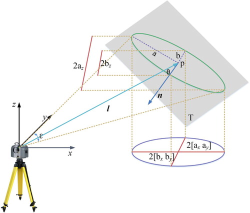
Assuming the beam emitted by the 3D terrestrial laser scanning system conforms to the Gaussian propagation, that is, the laser energy distribution in the footprint is normally distributed. Point position uncertainty resulting from the scanning geometry can be approximated by Eq. (5)(5) $${\sigma }_{xy}^{\text{geom}}=\frac{1}{3}\max \left(\left|\begin{array}{c}{a}_x\\ a_y\end{array}\right|,\left|\begin{array}{c}{b}_x\\ b_y\end{array}\right|\right),{\sigma }_z^{\text{geom}}=\frac{1}{3}\max \left(\left|a_z\right|,\left|b_z\right|\right)$$(5) (Schaer et al. 2007): (5) $${\sigma }_{xy}^{\text{geom}}=\frac{1}{3}\max \left(\left|\begin{array}{c}{a}_x\\ a_y\end{array}\right|,\left|\begin{array}{c}{b}_x\\ b_y\end{array}\right|\right),{\sigma }_z^{\text{geom}}=\frac{1}{3}\max \left(\left|a_z\right|,\left|b_z\right|\right)$$(5)

Where $a_x,$ $a_y,$ $a_z,$ $b_x,$ $b_y$ and $b_z$ are the projection length of the footprint semi-major axis $a$ and semi-minor axis $b$ on the x-axis, y-axis and z-axis, respectively. So, the total position uncertainty is ${\sigma }_{\text{total}}=\sqrt{{\sigma }_{xy}^2+{\sigma }_z^2}.$

First, the spatial rectangular coordinate $O-x^{\prime }{y}^{\prime }{z}^{\prime }$ at the laser origin $O$ is created, where the laser beam direction $\mathit{l}$ and the plane perpendicular to the laser beam direction are regarded as the z′-axis and the $x^{\prime }O{y}^{\prime }$ coordinate plane, respectively. The cone formed by the origin, laser direction, and beam divergence is expressed by Eq. (6)(6) $${z^{\prime }}^2={\left(\cot \epsilon /2\right)}^2\left({x^{\prime }}^2+{y^{\prime }}^2\right)$$(6) : (6) $${z^{\prime }}^2={\left(\cot \epsilon /2\right)}^2\left({x^{\prime }}^2+{y^{\prime }}^2\right)$$(6)

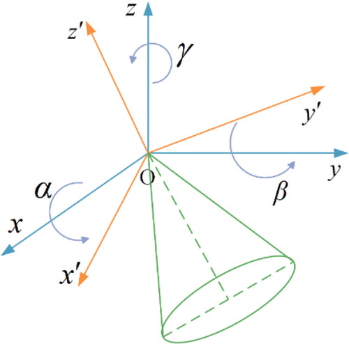
Figure 2 shows the position relationship between the $O-\mathit{xyz}$ and $O-x^{\prime }{y}^{\prime }{z}^{\prime }$ coordinate systems, the point coordinate can be calculated by Eq. (7)(7) $$\left(\begin{array}{c}{x}^{\prime }\\ y^{\prime }\\ z^{\prime }\end{array}\right)=\left[\begin{array}{ccc}\hspace{0.17em}\cos \hspace{0.17em}\beta \hspace{0.17em}\cos \hspace{0.17em}\gamma & \hspace{0.17em}\cos \hspace{0.17em}\beta \hspace{0.17em}\sin \hspace{0.17em}\gamma & -\hspace{0.17em}\sin \hspace{0.17em}\beta \\ -\hspace{0.17em}\cos \hspace{0.17em}\alpha \hspace{0.17em}\sin \hspace{0.17em}\gamma +\hspace{0.17em}\sin \hspace{0.17em}\mathrm{\alpha }\hspace{0.17em}\sin \hspace{0.17em}\beta \hspace{0.17em}\cos \hspace{0.17em}\gamma & \hspace{0.17em}\cos \hspace{0.17em}\alpha \hspace{0.17em}\cos \hspace{0.17em}\gamma +\hspace{0.17em}\sin \hspace{0.17em}\alpha \hspace{0.17em}\sin \hspace{0.17em}\beta \hspace{0.17em}\sin \hspace{0.17em}\gamma & \hspace{0.17em}\sin \hspace{0.17em}\alpha \hspace{0.17em}\cos \hspace{0.17em}\beta \\ \hspace{0.17em}\sin \hspace{0.17em}\alpha \hspace{0.17em}\sin \hspace{0.17em}\gamma +\hspace{0.17em}\cos \hspace{0.17em}\alpha \hspace{0.17em}\sin \hspace{0.17em}\beta \hspace{0.17em}\cos \hspace{0.17em}\gamma & -\hspace{0.17em}\sin \hspace{0.17em}\alpha \hspace{0.17em}\cos \hspace{0.17em}\gamma +\hspace{0.17em}\cos \hspace{0.17em}\alpha \hspace{0.17em}\sin \hspace{0.17em}\beta \hspace{0.17em}\sin \hspace{0.17em}\gamma & \hspace{0.17em}\cos \hspace{0.17em}\alpha \hspace{0.17em}\cos \hspace{0.17em}\beta \end{array}\right]\left(\begin{array}{c}x\\ y\\ z\end{array}\right)=\mathbf{C}\left(\begin{array}{c}x\\ y\\ z\end{array}\right)$$(7) : (7) $$\left(\begin{array}{c}{x}^{\prime }\\ y^{\prime }\\ z^{\prime }\end{array}\right)=\left[\begin{array}{ccc}\hspace{0.17em}\cos \hspace{0.17em}\beta \hspace{0.17em}\cos \hspace{0.17em}\gamma & \hspace{0.17em}\cos \hspace{0.17em}\beta \hspace{0.17em}\sin \hspace{0.17em}\gamma & -\hspace{0.17em}\sin \hspace{0.17em}\beta \\ -\hspace{0.17em}\cos \hspace{0.17em}\alpha \hspace{0.17em}\sin \hspace{0.17em}\gamma +\hspace{0.17em}\sin \hspace{0.17em}\mathrm{\alpha }\hspace{0.17em}\sin \hspace{0.17em}\beta \hspace{0.17em}\cos \hspace{0.17em}\gamma & \hspace{0.17em}\cos \hspace{0.17em}\alpha \hspace{0.17em}\cos \hspace{0.17em}\gamma +\hspace{0.17em}\sin \hspace{0.17em}\alpha \hspace{0.17em}\sin \hspace{0.17em}\beta \hspace{0.17em}\sin \hspace{0.17em}\gamma & \hspace{0.17em}\sin \hspace{0.17em}\alpha \hspace{0.17em}\cos \hspace{0.17em}\beta \\ \hspace{0.17em}\sin \hspace{0.17em}\alpha \hspace{0.17em}\sin \hspace{0.17em}\gamma +\hspace{0.17em}\cos \hspace{0.17em}\alpha \hspace{0.17em}\sin \hspace{0.17em}\beta \hspace{0.17em}\cos \hspace{0.17em}\gamma & -\hspace{0.17em}\sin \hspace{0.17em}\alpha \hspace{0.17em}\cos \hspace{0.17em}\gamma +\hspace{0.17em}\cos \hspace{0.17em}\alpha \hspace{0.17em}\sin \hspace{0.17em}\beta \hspace{0.17em}\sin \hspace{0.17em}\gamma & \hspace{0.17em}\cos \hspace{0.17em}\alpha \hspace{0.17em}\cos \hspace{0.17em}\beta \end{array}\right]\left(\begin{array}{c}x\\ y\\ z\end{array}\right)=\mathbf{C}\left(\begin{array}{c}x\\ y\\ z\end{array}\right)$$(7)

Where $\alpha ,$ $\beta$ and $\gamma$ are the rotation angle of the cone axis around the x-axis, y-axis and z-axis, respectively. For brevity, let $\mathbf{C}=\left[\begin{array}{ccc}{\mathbf{C}}_{11}& {\mathbf{C}}_{12}& {\mathbf{C}}_{13}\\ {\mathbf{C}}_{21}& {\mathbf{C}}_{22}& {\mathbf{C}}_{23}\\ {\mathbf{C}}_{31}& {\mathbf{C}}_{32}& {\mathbf{C}}_{33}\end{array}\right],$ So (8) $${\mathbf{C}}^{-1}=\frac{\left[\begin{array}{ccc}{\mathbf{C}}_{22}{\mathbf{C}}_{33}-{\mathbf{C}}_{32}{\mathbf{C}}_{23}& {\mathbf{C}}_{32}{\mathbf{C}}_{13}-{\mathbf{C}}_{12}{\mathbf{C}}_{33}& {\mathbf{C}}_{12}{\mathbf{C}}_{23}-{\mathbf{C}}_{13}{\mathbf{C}}_{22}\\ {\mathbf{C}}_{23}{\mathbf{C}}_{31}-{\mathbf{C}}_{21}{\mathbf{C}}_{33}& {\mathbf{C}}_{11}{\mathbf{C}}_{33}-{\mathbf{C}}_{31}{\mathbf{C}}_{13}& {\mathbf{C}}_{21}{\mathbf{C}}_{13}-{\mathbf{C}}_{11}{\mathbf{C}}_{23}\\ {\mathbf{C}}_{21}{\mathbf{C}}_{32}-{\mathbf{C}}_{31}{\mathbf{C}}_{22}& {\mathbf{C}}_{12}{\mathbf{C}}_{31}-{\mathbf{C}}_{11}{\mathbf{C}}_{32}& {\mathbf{C}}_{11}{\mathbf{C}}_{22}-{\mathbf{C}}_{12}{\mathbf{C}}_{21}\end{array}\right]}{{\mathbf{C}}_{11}{\mathbf{C}}_{22}{\mathbf{C}}_{33}+{\mathbf{C}}_{12}{\mathbf{C}}_{23}{\mathbf{C}}_{31}+{\mathbf{C}}_{21}{\mathbf{C}}_{32}{\mathbf{C}}_{13}-{\mathbf{C}}_{13}{\mathbf{C}}_{22}{\mathbf{C}}_{31}-{\mathbf{C}}_{11}{\mathbf{C}}_{23}{\mathbf{C}}_{32}-{\mathbf{C}}_{12}{\mathbf{C}}_{21}{\mathbf{C}}_{33}}=\left[\begin{array}{ccc}{\mathbf{D}}_{11}& {\mathbf{D}}_{12}& {\mathbf{D}}_{13}\\ {\mathbf{D}}_{21}& {\mathbf{D}}_{22}& {\mathbf{D}}_{23}\\ {\mathbf{D}}_{31}& {\mathbf{D}}_{32}& {\mathbf{D}}_{33}\end{array}\right]$$(8)

Figure 2. The position relationship between the $O-\mathit{xyz}$ and $O-x^{\prime }{y}^{\prime }{z}^{\prime }$ coordinate systems.

Thus, the cone equation in the coordinate system $O-\mathit{xyz}$ can be expressed by Eq. (9)(9) $${\left({\mathbf{D}}_{31}x+{\mathbf{D}}_{32}y+{\mathbf{D}}_{33}z\right)}^2={\left(\cot \frac{\epsilon }{2}\right)}^2\left[{\left({\mathbf{D}}_{11}x+{\mathbf{D}}_{12}y+{\mathbf{D}}_{13}z\right)}^2+{\left({\mathbf{D}}_{21}x+{\mathbf{D}}_{22}y+{\mathbf{D}}_{23}z\right)}^2\right]$$(9) : (9) $${\left({\mathbf{D}}_{31}x+{\mathbf{D}}_{32}y+{\mathbf{D}}_{33}z\right)}^2={\left(\cot \frac{\epsilon }{2}\right)}^2\left[{\left({\mathbf{D}}_{11}x+{\mathbf{D}}_{12}y+{\mathbf{D}}_{13}z\right)}^2+{\left({\mathbf{D}}_{21}x+{\mathbf{D}}_{22}y+{\mathbf{D}}_{23}z\right)}^2\right]$$(9)

Considering that the tangent plane equation: (10) $$\left(x-x_p\right)n_x+\left(y-y_p\right)n_y+\left(z-z_p\right)n_z=0$$(10)

The intersection between the cone and tangent plane can be obtained by simultaneous Eqs. (9)(9) $${\left({\mathbf{D}}_{31}x+{\mathbf{D}}_{32}y+{\mathbf{D}}_{33}z\right)}^2={\left(\cot \frac{\epsilon }{2}\right)}^2\left[{\left({\mathbf{D}}_{11}x+{\mathbf{D}}_{12}y+{\mathbf{D}}_{13}z\right)}^2+{\left({\mathbf{D}}_{21}x+{\mathbf{D}}_{22}y+{\mathbf{D}}_{23}z\right)}^2\right]$$(9) and (10)(10) $$\left(x-x_p\right)n_x+\left(y-y_p\right)n_y+\left(z-z_p\right)n_z=0$$(10) . Furthermore, the projection length of the two main axes is calculated. Assuming that $q_1(x_{q_1},y_{q_1},z_{q_1}),$ $q_2(x_{q_2},y_{q_2},z_{q_2}),$ $r_1(x_{r_1},y_{r_1},z_{r_1})$ and $r_2(x_{r_2},y_{r_2},z_{r_2})$ are the endpoints of the two main axes. According to the law of sine, the distance $d_{p{q}_1}$ between the point $p$ and endpoint $q_1$ can be expressed by Eq. (11)(11) $$d_{p{q}_1}=\frac{\left|\mathit{l}\right|\hspace{0.17em}\tan \hspace{0.17em}\left(\epsilon /2\right)\hspace{0.17em}\sin \hspace{0.17em}\left(90-\epsilon /2\right)}{\hspace{0.17em}\sin \hspace{0.17em}\left(90-\epsilon /2+\theta \right)}=\frac{\left|\mathit{l}\right|\hspace{0.17em}\tan \hspace{0.17em}\left(\epsilon /2\right)\hspace{0.17em}\cos \hspace{0.17em}\left(\epsilon /2\right)}{\hspace{0.17em}\cos \hspace{0.17em}\left(\theta -\epsilon /2\right)}$$(11) : (11) $$d_{p{q}_1}=\frac{\left|\mathit{l}\right|\hspace{0.17em}\tan \hspace{0.17em}\left(\epsilon /2\right)\hspace{0.17em}\sin \hspace{0.17em}\left(90-\epsilon /2\right)}{\hspace{0.17em}\sin \hspace{0.17em}\left(90-\epsilon /2+\theta \right)}=\frac{\left|\mathit{l}\right|\hspace{0.17em}\tan \hspace{0.17em}\left(\epsilon /2\right)\hspace{0.17em}\cos \hspace{0.17em}\left(\epsilon /2\right)}{\hspace{0.17em}\cos \hspace{0.17em}\left(\theta -\epsilon /2\right)}$$(11)

Therefore, the endpoints of the main axis satisfy Eq. (12)(12) $$\{\begin{array}{c}(x_q-x_p)n_x+(y_q-y_p)n_y+(z_q-z_p)n_z=0\\ {(x_q-x_p)}^2+{(y_q-y_p)}^2+{(z_q-z_p)}^2=d_{p{q}_1}^2\\ {({\mathbf{D}}_{31}{x}_q+{\mathbf{D}}_{32}{y}_q+{\mathbf{D}}_{33}{z}_q)}^2={(\mathit{cot}\epsilon /2)}^2[{({\mathbf{D}}_{11}{x}_q+{\mathbf{D}}_{12}{y}_q+{\mathbf{D}}_{13}{z}_q)}^2+{({\mathbf{D}}_{21}{x}_q+{\mathbf{D}}_{22}{y}_q+{\mathbf{D}}_{23}{z}_q)}^2]\end{array}$$(12) : (12) $$\{\begin{array}{c}(x_q-x_p)n_x+(y_q-y_p)n_y+(z_q-z_p)n_z=0\\ {(x_q-x_p)}^2+{(y_q-y_p)}^2+{(z_q-z_p)}^2=d_{p{q}_1}^2\\ {({\mathbf{D}}_{31}{x}_q+{\mathbf{D}}_{32}{y}_q+{\mathbf{D}}_{33}{z}_q)}^2={(\mathit{cot}\epsilon /2)}^2[{({\mathbf{D}}_{11}{x}_q+{\mathbf{D}}_{12}{y}_q+{\mathbf{D}}_{13}{z}_q)}^2+{({\mathbf{D}}_{21}{x}_q+{\mathbf{D}}_{22}{y}_q+{\mathbf{D}}_{23}{z}_q)}^2]\end{array}$$(12)

Based on this, two endpoints of the footprint can be obtained. Furthermore, according to the relationship that the major axis is perpendicular to the minor axis, other endpoints can be calculated using Eq. (13)(13) $$\{\begin{array}{c}(x_r-x_p)n_x+(y_r-y_p)n_y+(z_r-z_p)n_z=0\\ (x_r-x_p)(x_q-x_p)+(y_r-y_p)(y_q-y_p)+(z_r-z_p)(z_q-z_p)=0\\ {({\mathbf{D}}_{31}{x}_r+{\mathbf{D}}_{32}{y}_r+{\mathbf{D}}_{33}{z}_r)}^2={(\mathit{cot}\epsilon /2)}^2[{({\mathbf{D}}_{11}{x}_r+{\mathbf{D}}_{12}{y}_r+{\mathbf{D}}_{13}{z}_r)}^2+{({\mathbf{D}}_{21}{x}_r+{\mathbf{D}}_{22}{y}_r+{\mathbf{D}}_{23}{z}_r)}^2]\end{array}$$(13) : (13) $$\{\begin{array}{c}(x_r-x_p)n_x+(y_r-y_p)n_y+(z_r-z_p)n_z=0\\ (x_r-x_p)(x_q-x_p)+(y_r-y_p)(y_q-y_p)+(z_r-z_p)(z_q-z_p)=0\\ {({\mathbf{D}}_{31}{x}_r+{\mathbf{D}}_{32}{y}_r+{\mathbf{D}}_{33}{z}_r)}^2={(\mathit{cot}\epsilon /2)}^2[{({\mathbf{D}}_{11}{x}_r+{\mathbf{D}}_{12}{y}_r+{\mathbf{D}}_{13}{z}_r)}^2+{({\mathbf{D}}_{21}{x}_r+{\mathbf{D}}_{22}{y}_r+{\mathbf{D}}_{23}{z}_r)}^2]\end{array}$$(13)

Once the endpoints coordinates are calculated, the point position uncertainty can be obtained using Eq. (5)(5) $${\sigma }_{xy}^{\text{geom}}=\frac{1}{3}\max \left(\left|\begin{array}{c}{a}_x\\ a_y\end{array}\right|,\left|\begin{array}{c}{b}_x\\ b_y\end{array}\right|\right),{\sigma }_z^{\text{geom}}=\frac{1}{3}\max \left(\left|a_z\right|,\left|b_z\right|\right)$$(5) . Furthermore, the high-accuracy point cloud model with low position uncertainty is constructed for subsequent deformation analysis.

2.2. Adaptive projection point cloud comparison

Although the M3C2 algorithm can achieve an accurate comparison of multi-temporal point clouds, it is difficult to determine the projection radius and depth for complex topography. Towards that end, an adaptive projection point cloud comparison (AP-PCC) algorithm is proposed.

Considering that the sampling point spacing expands with increasing measuring range and the point density distribution is closely related to the accuracy of the deformation analysis, the minimum point spacing is set to resample point clouds and balance the relationship between processing time and accuracy.

As shown in Figure 3, in the M3C2 algorithm, there are no valid deformation information is recorded for a smaller projection radius, especially where movement results in a new occlusion area in the second-temporal point cloud. Although the corresponding points in the two-temporal point clouds can be obtained by increasing the projection radius, it has a soothing effect, meaning that false change can be recorded in the surrounding area if the radius is much larger than the point spacing. Considering that the topographical undulation of the local study area is small, and the deformation information of the occlusion area can be approximated by the surrounding point cloud, the corresponding points of the multi-temporal point clouds are searched within a small projection radius. If a minimum number of points less than the estimated centroid is found, the projection radius increases at the depth until enough corresponding points are searched or the radius reaches a setting threshold determined by the size of the occlusion area.

Figure 3. Adaptive projection point cloud comparison (AP-PCC) algorithm.

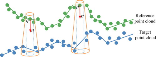
Like the projection radius, the projection depth is crucial for the deformation analysis. If setting a larger projection depth, the two-temporal point clouds contain multiple patches, which cannot accurately express true deformation information due to the corresponding points being the average value of different patch positions. On the contrary, there is no corresponding points that are searched in the case of setting a smaller projection depth. Therefore, the adaptive projection depth strategy is proposed. Specifically, the smaller depth value is adopted to search the corresponding points. If less than four points are found in the projection depth, the depth is increased until enough points participate in the corresponding point calculation, or the depth reaches the set threshold. After that, point sets that fall into the variable cylinder are acquired from the two-temporal point clouds, and the average position of the point sets projection on the cylinder axis is used to characterize the corresponding points.

The point cloud obtained through laser scanning technology is equivalent to many monitoring points arranged on the target, which are mutually influenced and related to each other, it is not enough to reflect the overall deformation trend and regularity of the deformed body only by processing single points. Considering the monitoring points on the same deformed block have similar regulations, the overall deformation prediction model can be established by multiple associated deformation points that are regarded as points on the same block using clustering algorithms. In our study, the k-means algorithm is used to perform cluster analysis on the distance of the corresponding points.

3. Experiments and results

3.1. Study area

Point cloud datasets acquired by terrestrial laser scanning technology are applied to evaluate the proposed method in this study (Figure 4), which includes a combined regular geometry (a) and landslides (b).

Figure 4. The study areas, (a) Combined regular geometry, (b) Landslides.

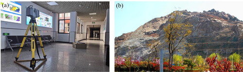
As shown in Figure 4(a), regular geometry consists of the carton, box and target sphere, where the length, width and height of the box are 31.8 cm, 23.8 cm and 4.6 cm, the diameter and base height of the target sphere are 14.5 cm and 0.7 cm, respectively, which can be regarded as the ground truth for deformation analysis. A total of four stations are set up, where the first two and the last two stations are in the same position. The single-carton data captured by stations 1 and 4 is regarded as the target point cloud, and the combined regular geometry data captured by stations 2 and 3 is defined as the reference point cloud.

The landslide is located in Shandong province, China. To verify the accuracy of the proposed method, the first two temporal point cloud is captured on the same day. The third-temporal point cloud is collected after the blasting and treatment. Table 1 shows the system specification and detailed dataset descriptions.

Table 1. Description of the datasets.

	Regular geometry		Landslide
	Reference point cloud	Target point cloud	First-temporal point cloud	Second-temporal point cloud	Third-temporal point cloud
Number of scans	2	2	5	5	3
Number of points	167,177	169,198	3,990,841	4,056,776	2,824,512
Accuracy
Range			2 mm
Angle			80 μrad
Point density
(points/m^2)	53,074	83,718	405	419	375

3.2. Point position uncertainty analysis based on scanning geometry

To analyze the influence of scanning geometry on the point cloud quality, various laser incident angles, scanning distances and beam divergence are set. Figure 5 shows the results of the point position uncertainty calculation.

Figure 5. Point position uncertainty is related to scanning geometry, where the solid line with a different color in each subplot indicates the changing trend of the point position uncertainty with the laser incident angle, scanning distance and beam divergence, respectively.

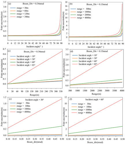
As shown in Figure 5(a,b), to analyze the effect of the incident angle on the position uncertainty, the scanning distance is set to 30 m, 60 m, 120 m and 340 m, the beam divergence is set to 0.34 mrad and 0.15 mrad, respectively, and the point position uncertainty is recorded with the laser incident angle changing (from 0° to 89°). When the beam divergence and scanning distance are fixed, the position uncertainty increases as the incident angle rises. Specifically, when the angle is in the range between 0° and 60°, the position uncertainty is only related to the scanning distance and beam divergence. However, if the incident angle is more than 60°, it increases exponentially. It is difficult to meet the measurement accuracy requirements when the angle reaches 80°.

In Figure 5(c), the effect of the scanning distance on the point position uncertainty can be seen. It changes linearly with the scanning distance when the beam divergence and incident angle are constant. As the incident angle increases, the uncertainty is more sensitive to the scanning distance. Specifically, when the measurement range is 300 m, the point position uncertainty at the incident angle of 30°, 60° and 85° are concentrated in the vicinity of 0, 8 cm, and 0.65 m, respectively. Figure 5(d) shows the changing trend of position uncertainty with scanning distance and incident angle when the beam divergence is 0.15 mrad, which is the same as that of Figure 5(c).

In the same way, the influence of the beam divergence on the position uncertainty is considered. As shown in Figure 5(e), as to the fixed scanning distance and incident angle, the uncertainty is positively correlated with the beam divergence. However, when the scanning distance is within 100 m and the incident angle is less than 60°, the uncertainty is concentrated around 0. Figure 5(f) presents the changing trend of position uncertainty with beam divergence and incident angle when the incident angle is 60°, the position uncertainty is more sensitive to the beam divergence with the scanning distance increase. In summary, these factors are positively correlated with position uncertainty.

3.3. Deformation analysis of the regular geometry point cloud

As mentioned earlier, the regular geometry point cloud is captured at four stations, and the point position uncertainty is calculated according to section 2.1.3, whose results are shown in Figure 6, where (a) to (d) corresponding to stations 1 to 4, respectively.

Figure 6. Point position uncertainty of the regular geometry point cloud, where (a) to (d) correspond to stations 1 to 4, respectively.

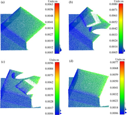
We can see that the point position uncertainty corresponding to four stations is low and is concentrated in the range between 0.5 and 1.5 mm, which is mainly because the scanning distance and incident angle are small. Therefore, the whole point cloud of the regular geometry is used to perform deformation analysis.

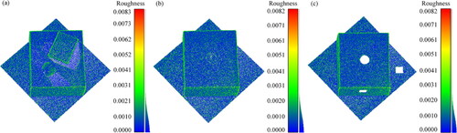
First, the plane features are extracted to transform stations 2 and 4 to the coordinate system where stations 1 and 3 are located, whose results are regarded as the reference and target point cloud, respectively. Then, the roughness of the multitemporal point cloud is calculated to determine the projection radius and depth, as shown in Figure 7(a,b), the roughness of the two-temporal point cloud is similar, with a mean about 0.9 mm. In addition, to evaluate the applicability of the proposed method in the area with large deformation or hole, the local data is removed manually from the target point cloud to simulate occlusion areas, whose roughness is shown in Figure 7(c).

Figure 7. The roughness of the multitemporal point cloud, where (a) to (c) is the roughness of the first to the third temporal point cloud, respectively.

Considering that stations 1 and 2 are captured at the same position, the reference and target point cloud are in the same coordinate system, there is no need to perform the coordinate unification of the multitemporal point cloud. The AP-PCC algorithm is implemented to calculate the deformation, whose results are depicted in Figure 8. Figure 8(a,b) shows the deformation analysis results of the first and second temporal point cloud using the M3C2 algorithm, where the projection search depths are 16 cm and 20 cm, respectively; Figure 8(c,d) is similar to Figure 8(a,b), but using the AP-PCC algorithm; Figure 8(e,f) shows the deformation analysis results of the first and third temporal point cloud using the M3C2 and AP-PCC algorithm, respectively. The projection search depth of the latter is 20 cm. It has to be noted that the normal vector neighborhood and initial projection radius are set to 12.5 cm and 2 cm, which are determined according to the point cloud surface roughness.

Figure 8. The deformation analysis results of the multitemporal point cloud. (a) and (b) are the deformation analysis results of the first and second temporal point cloud using the M3C2 algorithm, where the projection search depths are 16 cm and 20 cm, respectively; (c) and (d) are similar to (a) and (b), but using the AP-PCC algorithm; (e) and (f) is the deformation analysis results of the first and third temporal point cloud using the M3C2 and AP-PCC algorithm, respectively, the projection search depth of the latter is 20 cm.

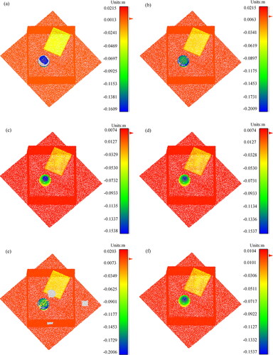
Comparing Figure 8(a) and Figure 8(b), the deformation magnitude varies with the projection depth using the M3C2 algorithm. Specifically, when the depths are 16 cm and 20 cm, the maximum deformation reaches 16.09 cm and 20.09 cm, respectively. However, the diameter of the target sphere is 15.50 cm. Therefore, the difference with design value using the M3C2 algorithm reaches 4.59 cm, mainly because the normal direction of the target sphere surface is not strictly perpendicular to the carton, the wrong corresponding points from the target point cloud is searched and the deformation information is overestimated. For the AP-PCC algorithm, the deformation magnitude is not affected by the parameter. Regardless of the projection depth set to 16 cm or 20 cm, the maximum deformation magnitude is 15.4 cm, and the difference to the ground truth is 1 mm. Thus, we can conclude that the AP-PCC algorithm can obtain more accurate deformation analysis results compared with the M3C2 algorithm.

In Figure 8(e,f), we can see that no valid deformation information in the hole areas can be acquired using the M3C2 algorithm, which is shown by grey points. While the point cloud characteristics surrounding the hole area are considered in the AP-PCC algorithm, which obtains the high accuracy deformation information of the complete point cloud compared with Figure 8(d).

3.4. Deformation analysis of the landslide point cloud

As shown in Figure 4(b), for capturing the complete landslide point cloud, the five stations are set far away from the landslide in the study area. After capturing multi-station point cloud, the point position uncertainty of each station is calculated, only the point cloud whose uncertainty is less than the set threshold is preserved. Then, the stations and multitemporal point clouds are transformed into a unified coordinate system. Finally, to verify the advantages of the AP-PCC algorithm in complex topography, the first and second temporal point cloud are analyzed using the C2C, C2M, M3C2 and AP-PCC algorithms, which are shown in Figure 9, where the first to third deformation analysis methods are carried out using the Cloud Compare software, the projection radius and depth are 0.3 m and 0.6 m, respectively.

Figure 9. Deformation analysis results of the first and second temporal point cloud using different methods. (a) to (d) are the detection results of the C2C, C2M, M3C2 and AP-PCC methods, respectively.

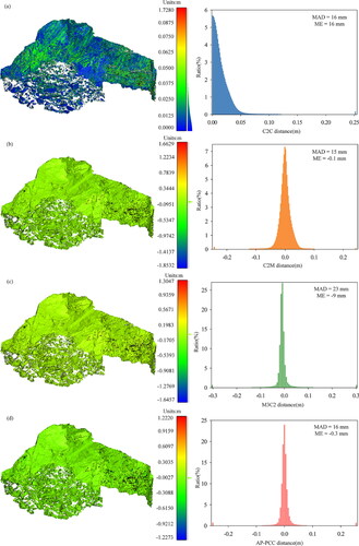
Theoretically, the first and second temporal point cloud are captured on the same day, there is no deformation occurring. However, due to the randomness of the laser scanning technology, the non-repeatability of the multitemporal point cloud and the roughness of the object surface, the distance of the corresponding points is not all zero. As shown in Figure 9(a), the distance between corresponding points using the C2C method is concentrated between the range of 0–5 cm, of which ME and MAD are 15.9 mm and 15.9 mm. However, this method can only calculate the relative distance between corresponding points and cannot reflect signed (–/+) displacement. Although the C2M method can reflect the change direction of the multitemporal point cloud, it is easy to generate sharp triangles in constructing the mesh and TIN model, which is not suitable for complex scanning scenes. Compared with C2M methods (ME and MAD are –0.1 mm and 14.8 mm), the distance between the corresponding points calculated using the M3C2 method is larger, its ME and MAD are –9.1 mm and 23 mm, which may be caused by inaccurate projection radius and depth settings. For the AP-PCC method, the ME and MAD of the distance between corresponding points are –0.3 mm and 16.2 mm. The ME and MAD values of the AP-PCC algorithm are similar to the C2M algorithm, and the distance between corresponding points is closer to zero. Therefore, the results indicate that the proposed method could obtain more accurate deformation information compared to other methods.

To verify the advantages of the proposed method in the scanning scene with a large deformation area, the M3C2 and AP-PCC method are used to analyze the first and third temporal point cloud, which are shown in Figure 10, the normal vector adjacent radius is 0.5882 m, the projection radius and depth are 0.2941 m and 20 m, respectively.

Figure 10. Deformation analysis results of the first and third landslide point cloud. (a) and (b) are the results using the M3C2 and AP-PCC methods, respectively; (b-i) cluster results; (b-ii) cluster distribution; (b-iii) point distribution.

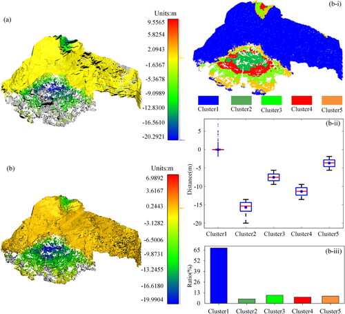
In Figure 10(a), the grey points on the top and bottom of the landslide represent the invalid deformation information, mainly because the corresponding points cannot be found using the small projection scale in the M3C2 algorithm. Although the phenomenon can be reduced by increasing the projection scale, it has a smooth effect on the sharp area. The deformation area can be accurately extracted using the AP-PCC method, which is shown in Figure 10(b), the maximum change of the landslide point cloud is located at the bottom area, about –20 m.

Furthermore, the deformation information is divided into cluster units by the k-means algorithm, which is shown in Figure 10(b-i) and Figure 10(b-ii), where the upper and lower bound of the rectangle box represent the 25th and 75th percentile of the ordinate, respectively. The solid line in the rectangle represents the median, and the upper and lower whisker line represents the maximum and minimum. In Figure 10(b-iii), we can see that the number of point cloud with means of 0, –4 m, –7 m, –12 m and –16 m accounted for 65%, 5%, 10%, 8% and 7% of the total point cloud, respectively. Thus, apart from the bottom of the landslide point cloud, most areas remain relatively stable, and the changes at the bottom of the point cloud might have been caused by the transportation of a large amount of gravel during the treatment process. Besides, there is a deformation area at the top of the landslide, about 10–13 m, where it needs to be reinforced and maintained to avoid disaster.

4. Discussion and conclusion

Considering that existing deformation analysis methods do not consider the influence of point cloud quality and it is difficult to search corresponding points in multitemporal measuring data, an accurate deformation analysis method based on point position uncertainty estimation and adaptive projection point cloud comparison is proposed. Two main improvements are implemented in this study.

1. Quantifying the point position uncertainty based on laser incidence angle, scanning distance and laser beam divergence. Although a series of literature about the impact of scanning geometry on point cloud quality can be found, they are focused on airborne laser scanning (ALS) systems with large beam diameters and full waveform information (Soudarissanane et al. 2011; Schaer et al., 2007). This study discusses the influence of TLS and survey properties on point cloud in complex environments. Results show that for terrestrial laser scanner with smaller beam divergence, the high accuracy point cloud can be captured even for a longer scanning distance if the laser incident angle is less than 60°. Whereas, for terrestrial laser scanner with larger laser beam divergence, if the laser scanning distance is less than 120 m, the high accuracy point cloud can be collected. It has to be noted the point position uncertainty analysis should be performed before multistation registration due to the scanning distance and angle change with the origin of the coordinates.

2. Proposing the adaptive projection point cloud comparison algorithm for the complex topography. To demonstrate the advantage of the AP-PCC algorithm, we compared the deformation analysis result with that of the C2C, C2M and M3C2 methods (Dimitri et al. 2013). As shown in Figure 8, the AP-PCC algorithm is not affected by the maximum projection depth and reduces the possibility of overestimating the deformation information. On the other hand, it can analyze deformation information of the occlusion area through the adaptive search radius. Comprehensive experiments represent that the mean error and mean absolute deviation of the distance between corresponding points are –0.3 mm and 16.2 mm, respectively, and the deformation information can be extracted in hole areas. It can be concluded that the proposed method can provide accurate deformation information for complex topography and an effective basis for terrain management.

Although the proposed method can extract high accuracy deformation information by point position uncertainty estimation and adaptive projection point cloud comparison, there are still some limitations to be considered. On one hand, scanner mechanism, atmospheric environment, object properties and scanning geometry should be considered comprehensively to construct a high accuracy point position uncertainty model (Soudarissanane et al. 2011) for estimating point cloud quality, but this study only analyzes the influence related to scanning geometry due to experimental conditions. On the other hand, the AP-PCC algorithm can obtain accurate deformation information for topography monitoring, and it is necessary to explore whether this method can be applied to other safety monitoring fields, such as large-scale structures and underground mining.

Data availability

The data that support the findings of this study are available from the corresponding author upon reasonable request.

Disclosure statement

No potential conflict of interest was reported by the authors.

Additional information

Funding

This study was supported by High-end Foreign Experts Recruitment Plan of China and Lunan Institute Open Fund.

References

- Abellán A, Calvet J, Vilaplana JM, Blanchard J. 2010. Detection and spatial prediction of rockfalls by means of terrestrial laser scanner monitoring. Geomorphology. 119(3–4):162–171.
- Abellán A, Jaboyedoff M, Oppikofer T, Oppikofer T, Vilaplana JM. 2009. Detection of millimetric deformation using a terrestrial laser scanner: experiment and application to a rockfall event. Nat Hazards Earth Syst Sci. 9(2):365–372.
- Alam MS, Kumar D, Chatterjee RS. 2022. Improving the capability of integrated DInSAR and PSI approach for better detection, monitoring, and analysis of land surface deformation in underground mining environment. Geocarto Int. 37(12):3607–3641.
- Anders K, Marx S, Boike J, Herfort B, Wilcox EJ, Langer M, Marsh P, Höfle B. 2020. Multitemporal terrestrial laser scanning point clouds for thaw subsidence observation at Arctic permafrost monitoring sites. Earth Surf Process Landforms. 45(7):1589–1600.
- Chen X, Yu K, Wu H. 2018. Determination of minimum detectable deformation of terrestrial laser scanning based on error entropy model. IEEE Trans Geosci Remote Sensing. 56(1):105–116.
- Dimitri L, Nicolas B, Jerome L. 2013. Accurate 3D comparison of complex topography with terrestrial laser scanner: application to the Rangitikei Canyon (N-Z). ISPRS J Photogramm Remote Sens. 82:10–26.
- Fey C, Wichmann V. 2017. Long-range terrestrial laser scanning for geomorphological change detection in alpine terrain – handling uncertainties. Earth Surf Process Landforms. 42(5):789–802.
- Girardeau-Montaut D, Roux M, Marc R, Thibault G. 2005. Change detection on points cloud data acquired with a ground laser scanner, International Archives of Photogrammetry, Remote Sensing and Spatial Information Sciences. 36.
- Kasperski J, Delacourt C, Allemand P, Potherat P, Jaud M, Varrel E. 2010. Application of a terrestrial laser scanner (TLS) to the study of the Séchilienne landslide (Isère, France). Remote Sens. 2(12):2785–2802.
- Huang D, Gu DM, Song YX, Cen DF, Zeng B. 2018. Towards a complete understanding of the triggering mechanism of a large reactivated landslide in the Three Gorges Reservoir. Eng Geol. 238:36–51.
- Huang R, Jiang L, Shen X, Dong Z, Zhou Q, Yang B, Wang H. 2019. An efficient method of monitoring slow-moving landslides with long-range terrestrial laser scanning: a case study of the Dashu landslide in the Three Gorges Reservoir Region, China. Landslides. 16(4):839–855.
- Hayakawa YS, Kusumoto S, Matta N. 2016. Application of terrestrial laser scanning for detection of ground surface deformation in small mud volcano (Murono, Japan). Earth Planets Space. 68:1–10.
- Jafari B, Khaloo A, Lattanzi D. 2017. Deformation tracking in 3D point clouds via statistical sampling of direct cloud-to-cloud distances. J Nondestr Eval. 36:65.
- Jack G, Williams KA, Lukas W, Vivien Z, Bernhard H. 2021. Multi-directional change detection between point clouds, ISPRS J Photogramm Remote Sens. 172:95–113.
- Kromer RA, Abellán A, Hutchinson DJ, Lato M, Chanut M-A, Dubois L, Jaboyedoff M. 2017. Automated terrestrial laser scanning with near-real-time change detection – monitoring of the Sechilienne landslide. Earth Surf Dyn. 5(2):293–310.
- Lichti D. 2007. Error modelling, calibration and analysis of an AM–CW terrestrial laser scanner system. ISPRS J Photogramm Remote Sen. 61(5):307–324.
- Lichti D, Gordon S. 2004. Error propagation in directly georeferenced terrestrial laser scanner point clouds for cultural heritage recording. Proceedings of FIG Working Week; Athens, Greece.
- Monserrat O, Crosetto M. 2008. Deformation measurement using terrestrial laser scanning data and least squares 3D surface matching. ISPRS J Photogramm Remote Sens. 63(1):142–154.
- Mukupa W, Roberts GW, Hancock CM, Al-Manasir K. 2017. A review of the use of terrestrial laser scanning application for change detection and deformation monitoring of structures. Surv Rev. 49(353):99–116.
- Riquelme AJ, Abellán A, Tomás R, Jaboyedoff M. 2014. A new approach for semi-automatic rock mass joints recognition from 3D point clouds. Comput Geosci. 68:38–52.
- Schürch P, Densmore A, Rosser N, Lim M, McArdell B. 2011. Detection of surface change in complex topography using terrestrial laser scanning: application to the Illgraben debris-flow channel. Earth Surf Process Landforms. 36(14):1847–1859.
- Soudarissanane S, Lindenbergh R, Menenti M, Teunissen P. 2011. Scanning geometry: influencing factor on the quality of terrestrial laser scanning points. ISPRS J Photogramm. Remote Sens. 66(4):389–399.
- Schaer P, Skaloud J, Landtwing S, Legat K. 2007. Accuracy estimation for laser point cloud including scanning geometry. The 5th International Symposium on Mobile Mapping Technology: Padua, Italy.
- Streletskiy DA, Shiklomanov NI, Little JD, Nelson FE, Brown J, Nyland KE, Klene AE. 2017. Thaw subsidence in undisturbed tundra landscapes, Barrow, Alaska, 1962–2015. Permafrost Periglac Process. 28(3):566–572.
- Sun W, Wang J, Jin F. 2020. An automatic coordinate unification method of multitemporal point clouds based on virtual reference datum detection. IEEE J Sel Top Appl Earth Observations Remote Sens. 13:3942–3950.
- Teza G, Galgaro A, Zaltron N, Genevois R. 2007. Terrestrial laser scanner to detect landslide displacement fields: a new approach. Int J Remote Sens. 28(16):3425–3446.
- Tiwari A, Narayan AB, Dwivedi R, Dikshit O, Nagarajan B. 2020. Monitoring of landslide activity at the Sirobagarh landslide, Uttarakhand, India, using LiDAR, SAR interferometry and geodetic surveys. Geocarto Int. 35(5):535–558.
- Williams JG, Anders K, Winiwarter L, Zahs V, Höfle B. 2021. Multi-directional change detection between point clouds. ISPRS J Photogramm Remote Sens. 172:95–113.
- Williams JG, Rosser NJ, Hardy RJ, Brain MJ, Afana AA. 2018. Optimising 4D approaches to surface change detection: improving understanding of Rockfall magnitude-frequency. Earth Surf Dyn. 6(1):101–119.
- Xu H, Li H, Yang X, Qi S, Zhou J. 2018. Integration of terrestrial laser scanning and NURBS modeling for the deformation monitoring of an earth-rock dam. Sensors. 19(1):22.
- Zhao X, Kargoll B, Omidalizarandi M, Xu X, Alkhatib H. 2018. Model selection for parametric surfaces approximating 3D point clouds for deformation analysis. Remote Sens. 10(4):634.